The Initial Mass Function and its Variation

Abstract

The observed distribution of IMF shapes can be understood as statistical sampling from a universal IMF and variations that result from stellar-dynamical processes. However, young star clusters appear to have an IMF biased towards low-mass stars when compared to the Galactic disk IMF, which comprises an average populated by star-formation episodes occurring Gyrs ago. In addition to this tentative but exciting deduction, this text outlines some of the stumbling blocks hindering the production of rigorous IMF determinations, and discusses the most robust evidence for structure in it. Also, it is stressed that an invariant IMF should not be expected.

Institut für Theoretische Physik und Astrophysik
Universität Kiel, D-24098 Kiel, Germany

1. Introduction

The stellar initial mass function (IMF) is one of the most fundamental distribution functions in astrophysics, and a large effort is being put into constraining its form and possible invariance. Much progress has been achieved since Salpeter published the first constraints in 1955. Most of the papers appearing in this field are observational in nature, which is necessary but not sufficient for providing the type of statistical sample necessary to address the two key questions, namely (1) what is the form of the IMF, and (2) does this form show unambiguous systematic variations with star-forming conditions?

In addition to the significant observational effort, low-cost modelling is crucial in distilling rigorous IMF properties from the many observational results offered to the community. For example, one young cluster may have a flatter IMF at low masses than another. Can such differences be attributed to different binary proportions, and if so, can these be explained by the clusters being in different stages of dynamical evolution, but starting with the same initial population? Does the observed mass-ratio distribution of Galactic-field binary systems reflect the initial conditions, or has it been substantially modified through stellar-dynamical evolution in young star clusters? Can bumps, wiggles and depressions in the observationally deduced IMF of a $\mbox{$\,\mathrel{\mathchoice{{\mbox{\lower 2.15277pt\vbox{\halign{$\mathsurround=0pt \displaystyle\hfil#\hfil$\cr<\crcr\sim\crcr}}}}}{{\mbox{\lower 2.15277pt\vbox{\halign{$\mathsurround=0pt \textstyle\hfil#\hfil$\cr<\crcr\sim\crcr}}}}}{{\mbox{\lower 2.15277pt\vbox{\halign{$\mathsurround=0pt \scriptstyle\hfil#\hfil$\cr<\crcr\sim\crcr}}}}}{{\mbox{\lower 2.15277pt\vbox{\halign{$\mathsurround=0pt \scriptscriptstyle\hfil#\hfil$\cr<\crcr\sim\crcr}}}}}}\,$}2$ Myr population be attributed to incomplete stellar physics, such as applying idealised non-rotating classical pre-main sequence contraction tracks of single stars to a real ensemble of fast-rotating magnetically active multiple stars that are still accreting and that retain a memory of their accretion history?

Without addressing these kinds of questions, which mean significant future theoretical stellar-dynamical and stellar-structure efforts in studying the IMF, any statements made about its shape are of limited scientific value. That this is a necessary complement to the observational effort for advancing knowledge on the IMF is demonstrated by the fact that apparent sub-structure in the IMF can be explained by fine-structure in the mass–luminosity relation of stars (Belikov et al. 1998; Kroupa 2001a), and that the Galactic-field binary-star properties can be unified with those of pre-main sequence stars if most stars form in embedded clusters, implying a surprising degree of universality of the primordial binary-star properties as well as of the IMF (Kroupa 1995; Kroupa, Aarseth & Hurley 2001).

After offering some technicalities in Section 2., the subject of the present text (see Kroupa 2001b for additional details) is to discuss the statistical properties of the available data (Section 3.), deduce possible evidence for a systematically varying IMF (Section 4.), and to point to particularly interesting questions that follow from the observational data and the modelling thereof (Section 5.).

2. The functional form and generating function

The number of stars in the mass interval $m$ to $m+dm$ is $\xi(m)\,dm$. Which particular functional form best approximates the IMF, $\xi(m)$, is very much open to debate. The multi-part power-law IMF has the merit that it is an easy analytical tool for describing the IMF over broad mass-ranges, allowing controlled variation of various parts of the IMF, such as what effects different relative numbers of massive stars have on star-cluster evolution without changing the form of the LF for low-mass stars. Also, the multi-part power-law IMF is easily transformed to the mass-generating function, which allows efficient creation of theoretical stellar populations.

Ensuring continuity leads to

$$\xi(m)=k\left\{\begin{array}[]{l@{\quad\quad,\quad}l}\left({m\over m_{\rm H}}\right)^{-\alpha_{0}}&m_{l}<m\leq m_{\rm H},\\ \left({m\over m_{\rm H}}\right)^{-\alpha_{1}}&m_{\rm H}<m\leq m_{0},\\ \left[\left({m_{0}\over m_{\rm H}}\right)^{-\alpha_{1}}\right]\left({m\over m_{0}}\right)^{-\alpha_{2}}&m_{0}<m\leq m_{1},\\ \left[\left({m_{0}\over m_{\rm H}}\right)^{-\alpha_{1}}\left({m_{1}\over m_{0}}\right)^{-\alpha_{2}}\right]\left({m\over m_{1}}\right)^{-\alpha_{3}}&m_{1}<m\leq m_{2},\\ \left[\left({m_{0}\over m_{\rm H}}\right)^{-\alpha_{1}}\left({m_{1}\over m_{0}}\right)^{-\alpha_{2}}\left({m_{2}\over m_{1}}\right)^{-\alpha_{3}}\right]\left({m\over m_{2}}\right)^{-\alpha_{4}}&m_{2}<m\leq m_{u},\\ \end{array}\right.$$ (1)

where $k$ contains the desired scaling. Note that the present data only support a three-part power-law IMF (eqn 2 below).

If $N_{\rm tot}$ is the total number of stars in some star-formation event, then the IMF can be interpreted as a probability density, $p(m)=\xi(m)/N_{\rm tot}$. The probability of picking a stellar mass in the range $m$ to $m+dm$ becomes $dX=p(m)dm$, so that $\int_{m_{l}}^{m_{u}}p(m^{\prime})dm^{\prime}=1;X_{m_{l}}^{m}=\int_{m_{l}}^{m}p(m^{\prime})dm^{\prime}$. From this the generating function, $m(X)$, is derived, with $X$ a discrete random deviate distributed uniformly between 0 and 1. The normalisation condition gives $X_{l}^{\rm H},X_{\rm H}^{0},X_{0}^{1},X_{1}^{2},X_{2}^{u}$ with $1=X_{l}^{\rm H}+X_{\rm H}^{0}+X_{0}^{1}+X_{1}^{2}+X_{2}^{u}$. For example, if $X$ falls into the range $X_{l}^{\rm H}+X_{\rm H}^{0}<X\leq X_{l}^{\rm H}+X_{\rm H}^{0}+X_{0}^{1}$ (i.e. $m_{0}<m\leq m_{1}$), then the corresponding stellar mass is generated from $m(X)=\left[m_{0}^{1-\alpha_{2}}+\left(X-X_{l}^{\rm H}-X_{\rm H}^{0}\right){\left(1-\alpha_{2}\right)\,K\over\beta_{2}}\right]^{1\over 1-\alpha_{2}},$ where $\beta_{2}=m_{0}^{\alpha_{2}}\left(m_{\rm H}/m_{0}\right)^{\alpha_{1}}$ from eqn. 1, and $K=N_{\rm tot}/k$.

3. The empirical alpha-plot

An exciting way to summarise the many IMF estimates is the alpha-plot (Fig. 1) which displays the determinations of the IMF power-law indices, $\alpha$, over the average logarithm of the mass interval over which $\alpha$ is derived.

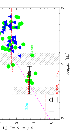
Figure 1.: The alpha-plot for Milky-Way (MW) and Large-Magellanic-Cloud (LMC) star-clusters and associations. Data are from the compilation of Scalo (1998). The horizontal dashed lines are the average IMF with estimated uncertainties (eqn 2), and the diagonal dot-dashed line is the popular Miller-Scalo (1979) IMF. From Kroupa (2001b). The figure can be obtained in colour from astro-ph/0009005.

Fig. 1 implies (additional details can be found in Kroupa 2001b):

1. The MW and LMC data show no systematic difference despite different average metallicities. $\alpha$ is thus at most weakly dependent on [Fe/H] for $m\mbox{$\,\mathrel{\mathchoice{{\mbox{\lower 2.15277pt\vbox{\halign{$\mathsurround=0pt \displaystyle\hfil#\hfil$\cr>\crcr\sim\crcr}}}}}{{\mbox{\lower 2.15277pt\vbox{\halign{$\mathsurround=0pt \textstyle\hfil#\hfil$\cr>\crcr\sim\crcr}}}}}{{\mbox{\lower 2.15277pt\vbox{\halign{$\mathsurround=0pt \scriptstyle\hfil#\hfil$\cr>\crcr\sim\crcr}}}}}{{\mbox{\lower 2.15277pt\vbox{\halign{$\mathsurround=0pt \scriptscriptstyle\hfil#\hfil$\cr>\crcr\sim\crcr}}}}}}\,$}3\,M_{\odot}$.
   

2. The IMF steepens progressively with increasing mass.
   

3. $\alpha$ appears to become constant near the Salpeter value for $m\mbox{$\,\mathrel{\mathchoice{{\mbox{\lower 2.15277pt\vbox{\halign{$\mathsurround=0pt \displaystyle\hfil#\hfil$\cr>\crcr\sim\crcr}}}}}{{\mbox{\lower 2.15277pt\vbox{\halign{$\mathsurround=0pt \textstyle\hfil#\hfil$\cr>\crcr\sim\crcr}}}}}{{\mbox{\lower 2.15277pt\vbox{\halign{$\mathsurround=0pt \scriptstyle\hfil#\hfil$\cr>\crcr\sim\crcr}}}}}{{\mbox{\lower 2.15277pt\vbox{\halign{$\mathsurround=0pt \scriptscriptstyle\hfil#\hfil$\cr>\crcr\sim\crcr}}}}}}\,$}0.5\,M_{\odot}$.
   

4. For $0.1-1\,M_{\odot}$ the cluster data are beautifully consistent with the Galactic-field IMF obtained from detailed star-count analysis using different mass-luminosity relations and corrected for unresolved binaries. Note that the Galactic-field IMF is especially tightly constrained for $0.5\mbox{$\,\mathrel{\mathchoice{{\mbox{\lower 2.15277pt\vbox{\halign{$\mathsurround=0pt \displaystyle\hfil#\hfil$\cr<\crcr\sim\crcr}}}}}{{\mbox{\lower 2.15277pt\vbox{\halign{$\mathsurround=0pt \textstyle\hfil#\hfil$\cr<\crcr\sim\crcr}}}}}{{\mbox{\lower 2.15277pt\vbox{\halign{$\mathsurround=0pt \scriptstyle\hfil#\hfil$\cr<\crcr\sim\crcr}}}}}{{\mbox{\lower 2.15277pt\vbox{\halign{$\mathsurround=0pt \scriptscriptstyle\hfil#\hfil$\cr<\crcr\sim\crcr}}}}}}\,$}m\mbox{$\,\mathrel{\mathchoice{{\mbox{\lower 2.15277pt\vbox{\halign{$\mathsurround=0pt \displaystyle\hfil#\hfil$\cr<\crcr\sim\crcr}}}}}{{\mbox{\lower 2.15277pt\vbox{\halign{$\mathsurround=0pt \textstyle\hfil#\hfil$\cr<\crcr\sim\crcr}}}}}{{\mbox{\lower 2.15277pt\vbox{\halign{$\mathsurround=0pt \scriptstyle\hfil#\hfil$\cr<\crcr\sim\crcr}}}}}{{\mbox{\lower 2.15277pt\vbox{\halign{$\mathsurround=0pt \scriptscriptstyle\hfil#\hfil$\cr<\crcr\sim\crcr}}}}}}\,$}1\,M_{\odot}$.
   

5. The scatter in $\alpha$ is small for $m\mbox{$\,\mathrel{\mathchoice{{\mbox{\lower 2.15277pt\vbox{\halign{$\mathsurround=0pt \displaystyle\hfil#\hfil$\cr<\crcr\sim\crcr}}}}}{{\mbox{\lower 2.15277pt\vbox{\halign{$\mathsurround=0pt \textstyle\hfil#\hfil$\cr<\crcr\sim\crcr}}}}}{{\mbox{\lower 2.15277pt\vbox{\halign{$\mathsurround=0pt \scriptstyle\hfil#\hfil$\cr<\crcr\sim\crcr}}}}}{{\mbox{\lower 2.15277pt\vbox{\halign{$\mathsurround=0pt \scriptscriptstyle\hfil#\hfil$\cr<\crcr\sim\crcr}}}}}}\,$}0.8\,M_{\odot}$.
   

6. The scatter is large but constant and apparently non-Gaussian for $m\mbox{$\,\mathrel{\mathchoice{{\mbox{\lower 2.15277pt\vbox{\halign{$\mathsurround=0pt \displaystyle\hfil#\hfil$\cr>\crcr\sim\crcr}}}}}{{\mbox{\lower 2.15277pt\vbox{\halign{$\mathsurround=0pt \textstyle\hfil#\hfil$\cr>\crcr\sim\crcr}}}}}{{\mbox{\lower 2.15277pt\vbox{\halign{$\mathsurround=0pt \scriptstyle\hfil#\hfil$\cr>\crcr\sim\crcr}}}}}{{\mbox{\lower 2.15277pt\vbox{\halign{$\mathsurround=0pt \scriptscriptstyle\hfil#\hfil$\cr>\crcr\sim\crcr}}}}}}\,$}3\,M_{\odot}$.
   

7. The shaded regions indicate mass-ranges that are particularly prone to errors. At the low-mass end the long contraction times to the main sequence make mass estimates very difficult when the ages are unknown. Near $2\,M_{\odot}$ evolution along and off the main sequence becomes problematical for the same reason, and stars in this mass range are typically the most massive in the cluster samples entering Fig. 1, and thus especially prone to stellar-dynamical biases (mass segregation and ejections). Not much emphasis is thus placed on the large observational scatter in the shaded region near $2\,M_{\odot}$.
   

Based on the above and previous work, Kroupa (2001b) approximates the average Galactic-field IMF with

$$\begin{array}[]{l@{\quad\quad,\quad}l}\alpha_{0}=+0.3\pm 0.7&0.01\leq m/M_{\odot}<0.08,\\ \alpha_{1}=+1.3\pm 0.5&0.08\leq m/M_{\odot}<0.50,\\ \alpha_{2}=+2.3\pm 0.3&0.50\leq m/M_{\odot},\\ \end{array}$$ (2)

($\alpha_{4}=\alpha_{3}=\alpha_{2}$, the uncertainties reflect 95–99 per cent confidence intervals). This is an average because the Galactic-field is composed of many star-formation events that occurred Gyrs ago. Note that Salpeter (1955) estimated $\alpha=2.35$ for stars in the mass interval $0.4-10\,M_{\odot}$. Any confident variation of the IMF should be evident in significant departures from eqn 2.

4. A systematically varying IMF

The MW clusters plotted in Fig. 1 are between a few and 100 Myr old, and thus sample the latest episode of star-formation in the MW disc near the solar circle. The immediate but naive conclusion follows that the IMF remained the same over the age of the Galactic disc, at least to within the uncertainties apparent in Fig. 1. Perhaps this would not be surprising if most stars form in clusters (Kroupa 1995). However, what is the origin of the scatter of $\alpha$ values?

4.1. The theoretical alpha-plot

To address this problem, a large library of stellar-dynamical models was evolved for 150 Myr using a modified version of Aarseth’s (1999) Nbody6 code (costing a few months of CPU time on standard desk-top computers) of binary-rich clusters that have initially the same large central density (and thus the same crossing time) as the Orion Nebula Cluster, but different number of stars ($N=800,3000,10^{4}$). Stellar evolution is included and the initial binary-properties are consistent with pre-main sequence constraints. Stars are initially paired randomly from the IMF (eqn 2), but the mass-ratio distribution is rapidly depleted of low-mass companions. The MFs in the inner and outer regions of the clusters are constructed at 3 Myr and 70 Myr counting the masses of systems (single stars and remaining binaries) giving the system MF. Theoretical alpha-plots are generated to study the scatter in $\alpha$ values.

The resulting data are combined in Fig. 2. It is evident that the scatter is reproduced, it being approximately constant for $m\mbox{$\,\mathrel{\mathchoice{{\mbox{\lower 2.15277pt\vbox{\halign{$\mathsurround=0pt \displaystyle\hfil#\hfil$\cr>\crcr\sim\crcr}}}}}{{\mbox{\lower 2.15277pt\vbox{\halign{$\mathsurround=0pt \textstyle\hfil#\hfil$\cr>\crcr\sim\crcr}}}}}{{\mbox{\lower 2.15277pt\vbox{\halign{$\mathsurround=0pt \scriptstyle\hfil#\hfil$\cr>\crcr\sim\crcr}}}}}{{\mbox{\lower 2.15277pt\vbox{\halign{$\mathsurround=0pt \scriptscriptstyle\hfil#\hfil$\cr>\crcr\sim\crcr}}}}}}\,$}1\,M_{\odot}$. The unsettling finding, however, is that the system MFs show systematically smaller mean $\alpha$ for $0.1<m<1\,M_{\odot}$ than the input IMF (eqn 2). The bias amounts to $\Delta\alpha\approx 0.5$.

Figure 2.: The theoretical alpha-plot. From Kroupa (2001b). $\alpha$ is measured using least-squares fitting to segments of the MF that have the average log-masses indicated by the discrete values.

The binary proportion, $f$, decreases on the same time-scale in all clusters because they have the same crossing time. By a few Myr the binary population stabilises near $f=0.4-0.5$ depending on the initial number of stars in the cluster. For BDs $f\approx 0.2$ owing to their small binding energy. Real clusters are likely to have a larger $f$ (e.g. Kähler finds that $f\approx 0.7$ is possible for the Pleiades cluster), which would not be surprising given that the present models start from a very dense initial state leading to efficient binary disruption. Thus, if anything, the bias in $\alpha$ is likely to be underestimated with the present calculations.

4.2. Implications

The cluster and association data plotted in Fig. 1 are not corrected for unseen companion stars. The implication is that these data must be systematically larger by at least $\Delta\alpha=0.5$ for low-mass stars. The bias is nearly negligible for BDs because they develop a small binary proportion and most BDs in stellar systems are disrupted from their stellar primaries. Thus, present-day star-formation seems to be producing more low-mass stars today than when most of the Galactic disk formed. The revised, present-day star-formation IMF thus reads

$$\begin{array}[]{l@{\quad\quad,\quad}l}\alpha_{0}=+0.3\pm 0.7&0.01\leq m/M_{\odot}<0.08,\\ \alpha_{1}=+1.8\pm 0.5&0.08\leq m/M_{\odot}<0.50,\\ \alpha_{2}=+2.7\pm 0.3&0.50\leq m/M_{\odot}<1.00,\\ \alpha_{3}=+2.3\pm 0.3&1.00\leq m/M_{\odot},\\ \end{array}$$ (3)

with $\alpha_{4}=\alpha_{3}$.

5. Important questions

1. Is it true, that the Galactic disk is now producing more low-mass stars than at an earlier epoch (eqn 3)? The most obvious physical parameter that changes with time is the overall metallicity and thus rate of cooling of a molecular cloud. Theoretical arguments lead to the expectation that such a variation ought to be the case, although it’s magnitude is uncertain (Larson 1998).

   For this systematic effect to go away, the solar-neighbourhood IMF would need to be steeper than most available studies imply (Kroupa 2001a).
   

2. Fig. 2 shows that for $m\mbox{$\,\mathrel{\mathchoice{{\mbox{\lower 2.15277pt\vbox{\halign{$\mathsurround=0pt \displaystyle\hfil#\hfil$\cr>\crcr\sim\crcr}}}}}{{\mbox{\lower 2.15277pt\vbox{\halign{$\mathsurround=0pt \textstyle\hfil#\hfil$\cr>\crcr\sim\crcr}}}}}{{\mbox{\lower 2.15277pt\vbox{\halign{$\mathsurround=0pt \scriptstyle\hfil#\hfil$\cr>\crcr\sim\crcr}}}}}{{\mbox{\lower 2.15277pt\vbox{\halign{$\mathsurround=0pt \scriptscriptstyle\hfil#\hfil$\cr>\crcr\sim\crcr}}}}}}\,$}6\,M_{\odot}$ the theoretical $\alpha(m)$ data fall towards smaller values. This results from under-sampling near the maximum stellar mass, and may be an artefact of the present models. However, observational data probably also suffer from such an effect, the possible implication being that the true underlying IMF may steepen for $m\mbox{$\,\mathrel{\mathchoice{{\mbox{\lower 2.15277pt\vbox{\halign{$\mathsurround=0pt \displaystyle\hfil#\hfil$\cr>\crcr\sim\crcr}}}}}{{\mbox{\lower 2.15277pt\vbox{\halign{$\mathsurround=0pt \textstyle\hfil#\hfil$\cr>\crcr\sim\crcr}}}}}{{\mbox{\lower 2.15277pt\vbox{\halign{$\mathsurround=0pt \scriptstyle\hfil#\hfil$\cr>\crcr\sim\crcr}}}}}{{\mbox{\lower 2.15277pt\vbox{\halign{$\mathsurround=0pt \scriptscriptstyle\hfil#\hfil$\cr>\crcr\sim\crcr}}}}}}\,$}6\,M_{\odot}$.
   

3. The modelling by Sagar & Richtler (1991) demonstrates that for a high binary proportion among massive stars (massive primaries and secondaries), the IMF is steeper by as much as $\Delta\alpha=0.4$ or more. It is thus possible, that for $m\mbox{$\,\mathrel{\mathchoice{{\mbox{\lower 2.15277pt\vbox{\halign{$\mathsurround=0pt \displaystyle\hfil#\hfil$\cr>\crcr\sim\crcr}}}}}{{\mbox{\lower 2.15277pt\vbox{\halign{$\mathsurround=0pt \textstyle\hfil#\hfil$\cr>\crcr\sim\crcr}}}}}{{\mbox{\lower 2.15277pt\vbox{\halign{$\mathsurround=0pt \scriptstyle\hfil#\hfil$\cr>\crcr\sim\crcr}}}}}{{\mbox{\lower 2.15277pt\vbox{\halign{$\mathsurround=0pt \scriptscriptstyle\hfil#\hfil$\cr>\crcr\sim\crcr}}}}}}\,$}1\,M_{\odot}$, $\alpha\mbox{$\,\mathrel{\mathchoice{{\mbox{\lower 2.15277pt\vbox{\halign{$\mathsurround=0pt \displaystyle\hfil#\hfil$\cr>\crcr\sim\crcr}}}}}{{\mbox{\lower 2.15277pt\vbox{\halign{$\mathsurround=0pt \textstyle\hfil#\hfil$\cr>\crcr\sim\crcr}}}}}{{\mbox{\lower 2.15277pt\vbox{\halign{$\mathsurround=0pt \scriptstyle\hfil#\hfil$\cr>\crcr\sim\crcr}}}}}{{\mbox{\lower 2.15277pt\vbox{\halign{$\mathsurround=0pt \scriptscriptstyle\hfil#\hfil$\cr>\crcr\sim\crcr}}}}}}\,$}2.7$, keeping in mind the previous point.
   

4. What is the Galactic-field IMF for $m\mbox{$\,\mathrel{\mathchoice{{\mbox{\lower 2.15277pt\vbox{\halign{$\mathsurround=0pt \displaystyle\hfil#\hfil$\cr>\crcr\sim\crcr}}}}}{{\mbox{\lower 2.15277pt\vbox{\halign{$\mathsurround=0pt \textstyle\hfil#\hfil$\cr>\crcr\sim\crcr}}}}}{{\mbox{\lower 2.15277pt\vbox{\halign{$\mathsurround=0pt \scriptstyle\hfil#\hfil$\cr>\crcr\sim\crcr}}}}}{{\mbox{\lower 2.15277pt\vbox{\halign{$\mathsurround=0pt \scriptscriptstyle\hfil#\hfil$\cr>\crcr\sim\crcr}}}}}}\,$}1\,M_{\odot}$? We have no direct information on this! We only have constraints on the IMF for intermediate and massive stars for present-day star-formation in clusters and OB associations, and eqn 2 is pure speculation for $m>1\,M_{\odot}$ (the dichotomy problem stated in Kroupa 2001b).
   

5. So far not discussed, but very important, is the point made by a number of authors (e.g. Eisenhower 2001) that some star-bursts indicate IMFs that are top-heavy. How reliable is this evidence? This cannot be answered until high-precision stellar-dynamical models of realistic very young massive star-clusters that typically form en masse in star-bursts have become available, and the reliability of the stellar models for young massive stars are improved. Thus, for example, a kinematically decoupled core of massive stars may be embedded in a cluster that predominantly consists of low-mass stars. The core can have a velocity dispersion typical for the massive sub-population, but not indicative of the entire cluster. Available stellar-dynamical models of moderately massive clusters do indicate that mass segregation is very rapid, on the order of a few initial crossing times, so that by a few Myrs a decoupled core of OB stars may have formed in most massive clusters (Kroupa 2001c). Until stellar-dynamical libraries, such as is being constructed by Kroupa (2001c), are not analysed in this respect taking into account the observations, the statements on IMFs in star bursts remain all too speculative.
   

6. What is the physical basis for the structure evident in the IMF (flattening near 0.5 and $0.08\,M_{\odot}$, eqn 2)? Adams & Fatuzzo (1996), Padoan & Nordlund (2001), Klessen (2001b) and Bonnell et al. (2001) attempt various explanations.
   

6. Concluding remarks

The theoretical data presented in Fig. 2 imply that the scatter in the alpha-plot can be understood as being stochastic in nature (as also stressed by Elmegreen 1999), together with deviations caused by stellar-dynamical processes. It is surprising though that the observational data in Fig. 1 show a comparable distribution to the theoretical data plotted in Fig. 2, indicating that there are no additional stochastic effects and that the IMF is close to being invariant.

The bias through unresolved binary systems, however, implies that for low-mass stars the cluster-data require a present-day IMF that is systematically steeper than the solar-neighbourhood IMF. The argument leading to this deduction is simple: An average IMF is calculated from the cluster and association data in Fig. 1 giving eqn 2 (ignoring the Galactic-field constraints). This average IMF is used to construct theoretical alpha-plots of realistic cluster populations, leading to contradiction with the empirical data that are the basis for the input IMF. The systematic disagreement between the theoretical and empirical data imply that the true underlying IMF must be steeper for low-mass stars (eqn 3) than the assumed IMF (eqn 2), the latter also being the Galactic-field IMF.

This result opposes the cherished belief that the IMF is universal. But this conviction is not intuitive anyway, since the fundamental physics of star formation provides rather convincing arguments for variations. If the systematic variation is true, then it must be even more evident in extreme populations. Thus, metal-poorer populations ought to have an IMF with systematically smaller $\alpha$ for low-mass stars. While observations tentatively suggest this may be the case for globular clusters, the evidence is ambiguous, because dynamical evolution leads to the preferential loss of low-mass stars. The white-dwarf (WD) candidates in the Galactic halo may represent a very early phase of star-formation in the Galaxy, and the absence of associated low-mass stars that ought to still burn H suggests again the same sense of systematic evolution of the IMF. However, this evidence too is not yet rigorous, since the nature of the WD candidates must first be illuminated (Chabrier 1999).

Even within an embedded star-cluster systematic variations ought to occur, because near the high-density core of the cluster proto-stars interact if the proto-star collapse time-scale is comparable to or longer than the local cluster crossing time-scale. Thus, massive stars are expected to form near cluster centres (Bonnell, Bate & Zinnecker 1998; Klessen 2001a; Bonnell et al. 2001), which is also suggested by observation (e.g. Hillenbrand 1997) and the requirement of producing enough run-away OB stars (Kroupa 2001c). Once a massive star ignites, further star-formation is compromised through the explosively propagating HII region, which may affect the number of BDs and less massive objects, at least some of these possibly being unfinished stars. The sub-stellar part of the IMF should thus also show variations depending on environment, and a tentative hint at this has been reported (Luhman 2000). However, again it must be stressed that this evidence may be elusive because the stellar-dynamical models also lead to an apparent overabundance of BDs in dense regions simply because such clusters are dynamically evolved leading to many more star–BD and BD–BD systems having been disrupted (more BDs for the observer to see).

References

Aarseth, S. J. 1999, PASP, 111, 1333

Adams, F. C., Fatuzzo, M. 1996, ApJ, 464, 256

Belikov, A. N., Hirte, S., Meusinger, H., Piskunov, A. E. & Schilbach, E. 1998, A&A, 332, 575

Bonnell, I. A., Bate, M. R., Zinnecker, H. 1998, MNRAS, 298, 93

Bonnell, I. A., Clarke, C. J., Bate, M. R., Pringle, J. E. 2001, MNRAS, in press (astro-ph/0102121)

Chabrier G., 1999, ApJ, 513, L103

Eisenhauer, F. 2001, in Starbursts: Near and Far, eds. L.J. Tacconi and D. Lutz, in press (astro-ph/0101321)

Elmegreen, B. G. 1999, ApJ, 515, 323

Hillenbrand, L. A. 1997, AJ, 113, 1733

Kähler, H. 1999, A&A, 346, 67

Klessen, R. 2001a, ApJL, in press (astro-ph/0101277)

Klessen, R. 2001b, ApJ, submitted

Kroupa, P. 1995, MNRAS, 277, 1507

Kroupa, P. 2001a, in ASP Conf. Ser., Star2000: Dynamics of Star Clusters and the Milky Way, eds. S. Deiters, R. Spurzem, et al., in press (astro-ph/0011328)

Kroupa, P. 2001b, MNRAS, in press (astro-ph/0009005)

Kroupa, P. 2001c, in ASP Conf. Ser., IAU Symp.200: The Formation of Binary Stars, eds. H. Zinnecker, R. Mathieu, in press (astro-ph/0010347)

Kroupa, P., Aarseth, S. J., Hurley, J. 2001, MNRAS, in press (astro-ph/0009470)

Larson, R. B. 1998, MNRAS, 301, 569

Luhman, K. 2000, ApJ, 544, 1044

Miller, G. E., Scalo, J. M. 1979, ApJS, 41, 513

Muench, A. A., Lada, E. A., Lada, C. J. 2000, ApJ, 533, 358

Padoan, P., Nordlund, A. 2001, ApJ, submitted (astro-ph/0011465)

Sagar, R., Richtler, T. 1991, A&A, 250, 324

Salpeter, E. E. 1955, ApJ, 121, 161

Scalo, J. M. 1998, in ASP Conf. Ser. Vol. 142, The Stellar Initial Mass Function, eds. G. Gilmore & D. Howell (San Francisco: ASP), p.201