Constructing, characterizing, and simulating Gaussian and higher–order point distributions

Abstract

The definition and the properties of a Gaussian point distribution, in contrast to the well–known properties of a Gaussian random field are discussed. Constraints for the number density and the two–point correlation function arise. A simple method for the simulation of this so–called Gauss–Poisson point process is given and illustrated with an example. The comparison of the distribution of galaxies in the PSCz catalogue with the Gauss–Poisson process underlines the importance of higher–order correlation functions for the description for the galaxy distribution. The construction of the Gauss–Poisson point process is extended to the $n$–point Poisson cluster process, now incorporating correlation functions up to the $n$th–order. The simulation methods and constraints on the correlation functions are discussed for the $n$–point case and detailed for the three–point case. As another approach, well suited for strongly clustered systems, the generalized halo–model is discussed. The influence of substructure inside the halos on the two– and three–point correlation functions is calculated in this model.

I Introduction

Stochastic models are often used to describe physical phenomena. For spatial structures two broad classes of stochastic models have been established. One approach is based on random fields and the other one on random distributions of discrete objects, often only points, in space (see the contributions in [1] for recent applications and reviews). Stochastic point distributions are used to describe physical systems on vastly differing length–scales. The physical applications discussed in this article deal with the large–scale structures in the Universe formed by the distribution of galaxies. However, the methods are much more versatile.

Models for the dynamics of cosmic structures are often based on nonlinear partial differential equations for the mass density and velocity field. These models relate the initial mass density and velocity field, primarily modeled as Gaussian random fields, to the present day values of these fields. The nonlinear evolution leads to non–Gaussian features in the fields. However, observations supply us with the positions of galaxies in space. To compare theories with observations one has to relate fields with point distributions. Both deterministic or stochastic models have been used for this purpose so far (e.g. [2, 3]).

Pursuing a direct approach, the observed spatial distribution of galaxies (galaxy clusters etc.) is compared to models for random point sets. Only a few attempts towards a dynamics of galaxies as discrete objects have been made (see e.g. [4]), however stochastic models are quite common. Following the works by [5, 6, 7, 8], and [9] a purely stochastic description of the spatial distribution of galaxies as points in space is given in this article.

Models for stochastic point processes can be constructed using the physical interactions of the objects, typically leading to Gibbs processes (see e.g. [10, 11], and the generalizations by [12, 13, 14]). Another approach to construct point processes is based on purely geometrical considerations, e.g. points are randomly distributed on randomly placed line–segment (see [15, 16]). As a third possibility one can start from the characterization of point processes by the probability generating functional (p.g.fl.) and the expansion in terms of correlation functions. This is the way pursued in this work.

The simplest point process is a Poisson process showing no correlations at all. Since the galaxy distribution is highly clustered, a Poisson process is not a realistic model. The model with the next level of sophistication is a Gauss–Poisson process, the point distribution counterpart of a Gaussian random field. Whereas the properties of Gaussian random fields have been extensively studied, the Gauss–Poisson process has not been discussed in the cosmological literature in a systematic way. Some of the statistical properties of random fields directly translate to similar statistical properties of point distributions, but also important differences show up. The systematic inclusion of higher–order correlations, as well as the characterization, and the simulation algorithms for such point processes will be discussed.

Recently, a related class of stochastic models for the galaxy distribution, the halo–model, attracted some attention (see e.g. [17, 18, 19, 20]). These models are based on the assumption that galaxies are distributed inside correlated dark matter halos. Using the probability generating functional, the two– and three–point correlation function will be calculated for this model, extending the results by [21] to include the effects of halo–substructure.

The outline of this paper is as follows:
In Sect. II the properties of the probability generating functional (p.g.fl.) of a point process and the expansions in several types of correlation functions are briefly reviewed. The characterization of the Gauss–Poisson process is given in Sect. III, and the physical consequences of the constraints are discussed. The close relation to Poisson cluster) processes allows us to simulate a Gauss–Poisson process (see Appendix B 1. In Sect. IV simulations of the Gauss–Poisson processes and the line–segment process are used to show how the Gaussian approximation influences the $J(r)$-function, a statistic sensitive to higher–order correlations. A comparison of the galaxy distribution within the PSCz survey with a Gauss–Poisson processes illustrates the importance of higher–order correlations. In Sect. V the extension of the Gauss–Poisson point process to the $n$–point Poisson cluster process is discussed. Detailed results are derived for the three–point Poisson cluster process (the simulation recipe is give in Appendix B 2). The characterization of the general $n$–point process is discussed which is again detailed for the three–point case. Differences between a point process and a random field are highlighted in Sect. VI. Models for strongly correlated systems are mentioned in Sect. VII. The focus will be on the “halo model”. Using the formalism based on the p.g.fl., the correlation functions of the “halo model”, including the effects of halo–substructure, are calculated in Sect. VII B. In Sect. VIII some open problems are mentioned. An outlook is provided in Sect. IX. As an example the probability generating function (p.g.f.) of a random variable and its expansions in several kinds of moments is reviewed in Appendix A.

II Product densities, factorial cumulants, and the probability generating functional

Probability generating functionals (p.g.fl.’s), and their expansions in different kinds of correlation measures have been used to describe noise in time series (e.g. [22]) and the electro–magnetic cascades occurring in air–showers (e.g. [23]). They have been employed in the theory of liquids (e.g. [24]) and other branches of many–particle physics (e.g. [25]). The mathematical theory of p.g.fl.’s for point processes is nicely reviewed in the book of [26]. Stochastic methods based on p.g.f.’s have been introduced to cosmology by [5] (the p.g.fl. was presented by [27] in the discussion of this article), and became well–known following the work of [7] and [8]. Focusing on the factorial moments (the volume averaged $n$–point densities) and on count–in–cells, [9] discussed several expansions of the p.g.f.’s. In the following only “simple” point processes will be considered: at each position in space at most one object is allowed. This assumption is physically well justified for galaxies. Also, for quantum systems the methods should be refined (see e.g. [28] for fermionic (determinantal) point processes).

An intuitive way to characterize a point process is to use $n$th–product densities: $\varrho_{n}({\mathbf{x}}_{1},\ldots,{\mathbf{x}}_{n}){\rm d}V_{1}\cdots{\rm d}V_{n}$ is the probability of finding a point in each of the volume elements ${\rm d}V_{1}$ to ${\rm d}V_{n}$. For stationary and isotropic point fields $\varrho_{1}({\mathbf{x}})=\varrho$ is the mean number density, and the product density (with a slight abuse of notation) is $\varrho_{2}({\mathbf{x}}_{1},{\mathbf{x}}_{2})=\varrho_{2}(r)$ with $r=|{\mathbf{x}}_{1}-{\mathbf{x}}_{2}|$ being the separation of the two points. The factorial cumulants $c_{[n]}({\mathbf{x}}_{1},\ldots,{\mathbf{x}}_{n})$ are the irreducible or connected parts of the $n$th–product densities. E.g. for $n=2$

$$\varrho_{2}(r)=\varrho^{2}+c_{[2]}(r)=\varrho^{2}\Big{(}1+\xi_{2}(r)\Big{)},$$ (1)

and the second factorial cumulant $c_{[2]}(r)$ and the two–point correlation function $\xi_{2}(r)$ quantify the two–point correlations in excess of Poisson distributed points.

A systematic characterization of a point process is provided by the probability generating functional or a series of probability generating functions (see Appendix A). Equivalent to a random distribution of points in space, one considers a point process as a random counting measure. A realization is then a counting measure $N$, which assigns to each suitable set $A\subset{\mathbb{R}}^{d}$ the number of points $N(A)$ inside. For suitable functions $h({\mathbf{x}})$ one defines the probability generating functional of a point process via

$$G[h]={\mathbb{E}}\Bigg{[}\exp\Big{(}\int_{{\mathbb{R}}^{d}}N({\rm d}{\mathbf{x}})\log h({\mathbf{x}})\Big{)}\Bigg{]},$$ (2)

where ${\mathbb{R}}^{d}$ is the $d$–dimensional Euclidean space, and ${\mathbb{E}}$ is the expectation value, the ensemble average over realizations of the point process. Equivalently,

$$G[h]={\mathbb{E}}\Big{[}\prod\nolimits_{i}h({\mathbf{x}}_{i})\Big{]},$$ (3)

where ${\mathbf{x}}_{i}$ are the particle positions in a realization. Consider $k$ compact disjoint sets $A_{j}$, and let $n_{j}=N(A_{j})$ be the number of points inside $A_{j}$. The p.g.f. of the $k$-dimensional random vector $(n_{1},\cdots,n_{k})$ is then

$$P_{k}({\mathbf{z}})=P_{k}(z_{1},\ldots,z_{k})={\mathbb{E}}\bigg{[}\prod_{j=1}^{k}z_{j}^{n_{j}}\bigg{]}.$$ (4)

Together with a continuity requirement the knowledge of all finite dimensional p.g.f.’s $P_{k}$ determines the p.g.fl. $G$ and the point process completely (e.g. [26]). One obtains the p.g.f. $P_{k}({\mathbf{z}})=G[h^{\prime}]$ of the random vector ${\mathbf{z}}$ using

$$h^{\prime}({\mathbf{x}})=1-\sum_{j=1}^{k}(1-z_{j})\mbox{1l}_{A_{j}}({\mathbf{x}}),$$ (5)

where $\mbox{1l}_{A}({\mathbf{x}})$ is the indicator–function of the set $A$, with $\mbox{1l}_{A}({\mathbf{x}})=1$ for ${\mathbf{x}}\in{A}$ and zero otherwise. Several expansions of the p.g.fl. $G[h]$ are possible [26]. The expansion in terms of the product densities $\varrho_{n}$ (the Lebesgue densities of the factorial moment measures) reads

$$G[h+1]=1+\sum_{n=1}^{\infty}\frac{1}{n!}\int_{{\mathbb{R}}^{d}}{\rm d}{\mathbf{x}}_{1}\cdots\int_{{\mathbb{R}}^{d}}{\rm d}{\mathbf{x}}_{n}\\ \varrho_{n}({\mathbf{x}}_{1},\ldots,{\mathbf{x}}_{n})\ h({\mathbf{x}}_{1})\cdots h({\mathbf{x}}_{n}).$$ (6)

For the factorial cumulants $c_{[n]}$ or correlation functions $\xi_{n}$ one obtains

$$\log G[h+1] =\sum_{n=1}^{\infty}\frac{1}{n!}\int_{{\mathbb{R}}^{d}}{\rm d}{\mathbf{x}}_{1}\cdots\int_{{\mathbb{R}}^{d}}{\rm d}{\mathbf{x}}_{n}$$ (7)

$$\qquad c_{[n]}({\mathbf{x}}_{1},\ldots,{\mathbf{x}}_{n})\ h({\mathbf{x}}_{1})\cdots h({\mathbf{x}}_{n})$$ (8)

$$=\sum_{n=1}^{\infty}\frac{\varrho^{n}}{n!}\int_{{\mathbb{R}}^{d}}{\rm d}{\mathbf{x}}_{1}\cdots\int_{{\mathbb{R}}^{d}}{\rm d}{\mathbf{x}}_{n}$$ (9)

$$\qquad\xi_{n}({\mathbf{x}}_{1},\ldots,{\mathbf{x}}_{n})\ h({\mathbf{x}}_{1})\cdots h({\mathbf{x}}_{n}).$$ (10)

As a third possibility the p.g.fl. can be expanded around the origin:

$$G[h]=J_{0}+\sum_{n=1}^{\infty}\frac{1}{n!}\int_{{\mathbb{R}}^{d}}{\rm d}{\mathbf{x}}_{1}\cdots\int_{{\mathbb{R}}^{d}}{\rm d}{\mathbf{x}}_{n}\\ j_{n}({\mathbf{x}}_{1},\ldots,{\mathbf{x}}_{n})\ h({\mathbf{x}}_{1})\cdots h({\mathbf{x}}_{n}).$$ (11)

The Janossy densities $j_{n}({\mathbf{x}}_{1},\ldots,{\mathbf{x}}_{n}){\rm d}V_{1}\cdots{\rm d}V_{n}$ are the probability that there are exactly $n$ points, each in one of the volume elements ${\rm d}V_{1}$ to ${\rm d}V_{n}$. Convergence issues of these expansions are discussed in Sect. VIII.

III The Gauss–Poisson point process

For a stationary Poisson process with mean number density $\varrho$ the p.g.fl. is

$$\log G[h+1]=\varrho\int_{{\mathbb{R}}^{d}}{\rm d}{\mathbf{x}}\ h({\mathbf{x}}),$$ (12)

corresponding to a truncation of the expansion (7) after the first term. Truncating after the second term, one obtains the p.g.fl. for the Gauss–Poisson process [29, 30]

$$\log G[h+1]=\varrho\int_{{\mathbb{R}}^{d}}{\rm d}{\mathbf{x}}\ h({\mathbf{x}})+\\ +\frac{\varrho^{2}}{2}\int_{{\mathbb{R}}^{d}}{\rm d}{\mathbf{x}}\int_{{\mathbb{R}}^{d}}{\rm d}{\mathbf{y}}\ \xi_{2}(|{\mathbf{x}}-{\mathbf{y}}|)\ h({\mathbf{x}})h({\mathbf{y}}),$$ (13)

completely specified by its mean number density $\varrho$ and the two-point correlation function $\xi_{2}(r)$.

There is a close resemblance to random fields. For a homogeneous random field $\rho({\mathbf{x}})$ with mean ${\mathbb{E}}[\rho]=\overline{\rho}$ the density contrast is defined by $\delta({\mathbf{x}})=(\rho({\mathbf{x}})-\overline{\rho})/\overline{\rho}$. A homogeneous and isotropic Gaussian random field is stochastically fully specified by its mean $\overline{\rho}$ and its correlation function $\xi_{2}^{\delta}(|{\mathbf{x}}-{\mathbf{y}}|)={\mathbb{E}}[\delta({\mathbf{x}})\delta({\mathbf{y}})]$ [31]. Here, ${\mathbb{E}}$ is the average over realizations of the random field. The higher (connected) correlation functions $\xi_{n}^{\delta}=0$ with $n>2$ vanish. Similar the correlation functions $\xi_{n}$ for $n>2$ vanish in a Gauss–Poisson process. However, also important differences between a Gaussian random field and a Gauss–Poisson point process show up.

A Constraints on $\xi_{2}(r)$ and $\varrho$

A functional $G[h]$ defined by Eq. (13) is a p.g.fl. of a point process if and only if the $P_{k}({\mathbf{z}})$ as given in Eq. (4) are probability generating functions (p.g.f.’s). This will lead to restrictions on the two–point correlation function $\xi_{2}$ and the number density $\varrho$ as discussed by [29] and [30]. A $P_{k}({\mathbf{z}})$ given by Eq. (4) always has to be positive and monotonic increasing with each component $z_{i}$ of ${\mathbf{z}}$, and hence $\log P_{k}({\mathbf{z}})$ is non–decreasing in each component of ${\mathbf{z}}$. With Eqs. (4), (5) and (13) one gets

$$\frac{\partial\log P_{k}({\mathbf{z}})}{\partial z_{l}}=\varrho|A_{l}|+\\ +\varrho^{2}\sum_{j=1}^{k}\int_{A_{l}}{\rm d}{\mathbf{x}}\int_{A_{j}}{\rm d}{\mathbf{y}}\ \xi_{2}(|{\mathbf{x}}-{\mathbf{y}}|)(z_{j}-1)\geq 0$$ (14)

for any $z_{j}\geq 0$, where $|A_{l}|$ is the volume of the set $A_{l}$. The rather obvious constraint $\varrho\geq 0$ can be derived by setting $z_{j}=1$. For $z_{j}=1,j\neq i$, and either $z_{i}=0$ or $z_{i}\gg 1$ the following two non–trivial constraints emerge:

$$\frac{\varrho}{|A_{l}|}\ \int_{A_{l}}{\rm d}{\mathbf{x}}\int_{A_{i}}{\rm d}{\mathbf{y}}\ \xi_{2}(|{\mathbf{x}}-{\mathbf{y}}|)\leq 1$$ (15)

$$\int_{A_{l}}{\rm d}{\mathbf{x}}\int_{A_{i}}{\rm d}{\mathbf{y}}\ \xi_{2}(|{\mathbf{x}}-{\mathbf{y}}|)\geq\frac{-|A_{l}|}{\varrho(z_{i}-1)}\overset{z_{i}\rightarrow\infty}{\longrightarrow}0.$$ (16)

One can show that these two conditions provide a necessary and sufficient characterization of $\xi_{2}(r)$ and $\varrho$, to assure that $G[h]$, as given in Eq. (13), is a p.g.fl. [30].

Eq. (15) constrains the shape and normalization of the two–point correlation functions admissible in a Gauss–Poisson process. For $A_{l}=A=A_{i}$

$$\frac{\varrho}{|A|}\ \int_{A}{\rm d}{\mathbf{x}}\int_{A}{\rm d}{\mathbf{y}}\ \xi_{2}(|{\mathbf{x}}-{\mathbf{y}}|)=\overline{N}\ \sigma^{2}(A)\leq 1,$$ (17)

where $\sigma^{2}(A)$ are the fluctuations of count–in–cells in excess of a Poisson process, and $\overline{N}=\varrho|A|$ is the mean number of points inside the cell $A$. Hence, the total fluctuations of the number of points $N$ inside $A$ for a Gauss–Poisson process are

$${\mathbb{E}}[(N-\overline{N})^{2}]=\overline{N}+\overline{N}^{2}\ \sigma^{2}(A)\leq 2\ \overline{N},$$ (18)

and must not exceed twice the value of the fluctuations in a Poisson process ($\sigma^{2}=0$) for any domain $A$ considered. Another way of looking at constraint (15) is by taking $A_{l}$ as an infinitesimal volume element centered on the origin and $A_{j}$ equal to some volume $A$:

$$\varrho\ \int_{A}{\rm d}{\mathbf{y}}\ \xi_{2}(|{\mathbf{y}}|)\leq 1.$$ (19)

Consistent with Sect. III B this tells us that sitting on a point of the process on average at most one other point in excess of Poisson distributed points can be present.

Now consider two volume elements $A_{i}={\rm d}V_{i}$ and $A_{l}={\rm d}V_{l}$ separated by a distance of $r$, then Eq. (16) implies

$$\xi_{2}(r)\geq 0$$ (20)

Hence, only clustered point distributions can be modeled by a Gauss–Poisson process. Any zero crossing in $\xi_{2}(r)$ already indicates the presence of higher–order correlations.

B A Gauss–Poisson process as a Poisson cluster process

A Gauss–Poisson process can be interpreted as a simple Poisson cluster process. This is important for simulations (see Appendix B 1).

A Poisson cluster process is a two–stage point process. First one chooses Poisson distributed cluster centers, the “parents”, with number density $\varrho_{p}$ and then attaches a second point process – the cluster to each cluster center (the cluster center is not necessarily part of the point process). The p.g.fl. of a Poisson cluster process is then given by [26]

$$\log G[h]=\int_{{\mathbb{R}}^{d}}{\rm d}{\mathbf{x}}\ \varrho_{p}\big{(}G_{c}[h|{\mathbf{x}}]-1\big{)},$$ (21)

with $G_{c}[h|{\mathbf{x}}]$ being the p.g.fl.  of the point process forming the cluster at center ${\mathbf{x}}$. Now consider the p.g.fl.  of a cluster with at maximum two points (compare with Eq. (3)),

$$G_{c}[h|{\mathbf{x}}]=q_{1}({\mathbf{x}})h({\mathbf{x}})+q_{2}({\mathbf{x}})h({\mathbf{x}})\int_{{\mathbb{R}}^{d}}{\rm d}{\mathbf{y}}f(|{\mathbf{x}}-{\mathbf{y}}|)\ h({\mathbf{y}}),$$ (22)

where $q_{1}({\mathbf{x}})$ is the probability that only one point, the cluster center at ${\mathbf{x}}$, is entering the cluster, whereas $q_{2}({\mathbf{x}})$ is the probability that a second point is added. Clearly, $q_{1}({\mathbf{x}})+q_{2}({\mathbf{x}})=1$. The probability density $f(|{\mathbf{x}}-{\mathbf{y}}|)$ determines the distribution of the distance $|{\mathbf{x}}-{\mathbf{y}}|$ of the second point ${\mathbf{y}}$ to the cluster center, and is normalized according to $\int{\rm d}{\mathbf{z}}{}f(|{\mathbf{z}}|)=1$. By writing $f(|{\mathbf{x}}-{\mathbf{y}}|)$ one assumes that the probability density $f$ is symmetric in ${\mathbf{x}}$ and ${\mathbf{y}}$. Indeed, the p.g.fl. Eq. (21) is invariant under interchanging ${\mathbf{x}}$ and ${\mathbf{y}}$, and this assumption does not impose any restrictions. Using this expression and Eq. (21) one obtains

$$\log G[h+1]=\int_{{\mathbb{R}}^{d}}{\rm d}{\mathbf{x}}\ \varrho_{p}(1+q_{2}({\mathbf{x}}))\ h({\mathbf{x}})+\\ +\int_{{\mathbb{R}}^{d}}{\rm d}{\mathbf{x}}\int_{{\mathbb{R}}^{d}}{\rm d}{\mathbf{y}}\ \varrho_{p}q_{2}({\mathbf{x}})f(|{\mathbf{x}}-{\mathbf{y}}|)\ h({\mathbf{x}})h({\mathbf{y}}),$$ (23)

which equals the p.g.fl.  for the Gauss–Poisson process (13) for $\varrho=\varrho_{p}(1+q_{2})$ and $\xi_{2}(r)=2\frac{\varrho-\varrho_{p}}{\varrho^{2}}f(r)$. Hence every Gauss–Poisson process is a Poisson cluster process of the above type, and vice versa.

C Physical implications

From the preceding section one concludes that at maximum two points form a cluster in a Gauss–Poisson process. Therefore, no point distribution with large–scale structures can be modeled reliably with this kind of process. This has physical implications both for the galaxy distribution and percolating/critical systems.

More specific, from the observed galaxy distribution a scale–invariant two–point correlation function $\xi_{2}(r)=Ar^{-\gamma}$ with $\gamma\approx 1.8$ is deduced. Clearly such a correlation function does not satisfy the constraint (15). For $0<\gamma\leq 3$ a cut–off at large scales has to be introduced. For the galaxy distribution a cut–off at approximately 20$h^{-1}$Mpc is the lowest value which is roughly compatible with the observed two–point correlation function. Taking into account the observed number density of the galaxies, a cut–off even on this small scale does not help. Still the constraint (15) is strongly violated, indicating non negligible higher–order correlation functions (see also Sect. IV C). Similarly, a zero crossing or a negative $\xi_{2}(r)$ is violating the constraint (16) and also indicates that higher–order correlations are present. There are indications that the distribution of galaxies shows a negative $\xi_{2}(r)$ on some scale larger than 20$h^{-1}$Mpc, followed by a positive peak at approximately 120$h^{-1}$Mpc [32, 33, 34]. A Gauss–Poisson process is not able to describe these features in the distribution of galaxies and galaxy clusters.

Also a percolating cluster shows scale–invariant correlations. The correlation length, specifying e.g. the exponential cut–off of the two–point correlation function, is going to infinity near the percolation threshold. Therefore, the geometry of the largest cluster cannot be modeled with a Gauss–Poisson processes. Higher–order correlations are essential to describe the morphology of such a system. This again illustrates that the tails of the distributions, in this case the asymptotic behavior of the two–point correlation function is essential.

To summarize these results: already by looking at the two–point correlation function and the density one is able to exclude a Gauss–Poisson process as a model. However one cannot turn the argument around and show that a given point distribution is compatible with a Gauss–Poisson process using the two–point correlation function alone. There are point processes with higher–order correlations satisfying the constraints (15,16) as discussed in Sect. IV A.

IV Detecting deviations from a Gauss–Poisson process

After having outlined the basic theory of a Gauss–Poisson process, we discuss in this section how one can detect non–Gaussian features in a given point set.

A The line–segment process

First a two dimensional analytic example is studied. In the line–segment process points are randomly distributed on line segments which are themselves uniformly distributed in space and direction. The number of points per line segment is a Poisson random variable. According to [15], p. 286

$$\xi_{2}(r)=\begin{cases}\frac{1}{\pi l\varrho_{s}}\big{(}\frac{1}{r}-\frac{1}{l}\big{)}&\text{ for }r<l\\ 0&\text{ for }r\geq l;\end{cases}$$ (24)

$l$ is the length of the line segments and $\varrho_{s}$ is the mean number density of line segments; $l\varrho_{s}$, $\varrho/\varrho_{s}$, $\varrho$ denote the mean length density, the mean number of points per line segment (which can be smaller than one), and the mean number density in space, respectively. A similar model for the distribution of galaxies was discussed by [16]. On small scales $r\ll l$, $\xi_{2}(r)\propto r^{-1}$, qualitatively similar to the observed two–point correlation function in the galaxy distribution.

This structured point process incorporates higher–order correlations. In Fig. 1 the line–segment process is shown in comparison to a Gauss–Poisson process with the same two–point correlation function for the parameters $l=0.1$, $\varrho_{s}=201$, $\varrho=200$, and $\varrho=500$. A number density $\varrho>\varrho_{s}$ violates the constraint Eq. (15) and no Gauss–Poisson process equivalent on the two–point level to such a line–segment process exists.

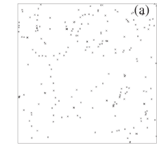
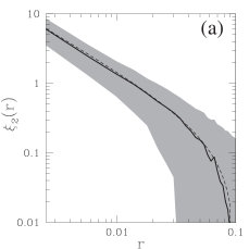
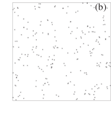
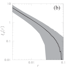
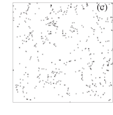
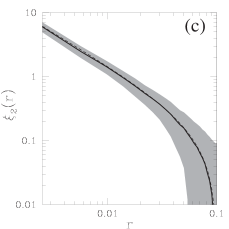
FIG. 1.: The plot (a) shows a realization of the line–segment process inside the unit square with number density $\varrho=200$ (for the other parameters see the text) and the corresponding two–point correlation function $\xi_{2}(r)$ ($r$ is in units of the box length): the dashed one–$\sigma$ area was determined from 1000 realizations, the theoretical value is given by the dashed line, nearly on top of the sample mean (solid line). The plot (b) shows a realization of the Gauss–Poisson process with $\varrho=200$ and the plot (c) a realization of the high density line–segment process with $\varrho=500$, both with the corresponding two–point correlation function.

B Detecting higher–order correlations

As can be seen from Fig. 1, the point processes are indistinguishable on the two–point level. For another example see [35, 36]. The differences between these point distributions can be investigated with statistical methods sensitive to higher–order correlations. One may use Minkowski functionals ([37], for reviews see [38, 39]), percolation techniques [40], the minimum spanning tree [41], a method sensitive to three–point correlations [42], or directly calculate the higher moments [43, 44, 45, 9]. In the following the $J$–function is used to quantify the higher–order clustering [46, 47, 48].

To define $J$-function the spherical contact distribution $F(r)$ is needed, i.e. the distribution function of the distances $r$ between an arbitrary point and the nearest object in the point set. $F(r)$ is equal to one minus the void–probability function: $F(r)=1-P_{0}(r)$. Another ingredient is the nearest neighbor distance distribution $G(r)$, defined as the distribution function of distances $r$ of an object in the point set to the nearest other point [49]. For a Poisson process the probability to find a point only depends on the mean number density $\varrho$, leading to the well–known result

$$G_{\rm P}(r)=1-\exp\big{(}-\varrho|B_{r}|\big{)}=F_{\rm P}(r),$$ (25)

where $|B_{r}|$ is the volume of a $d$–dimensional sphere with radius $r$. The ratio

$$J(r)=\frac{1-G(r)}{1-F(r)}$$ (26)

was suggested by [46] as a probe for clustering of a point distribution. For a Poisson distribution $J(r)=1$ follows directly from Eq. (25). A clustered point distribution implies $J(r)\leq 1$, whereas regular structures are indicated by $J(r)\geq 1$. As discussed in [47] one can express the $J(r)$ function in terms of the $n$–point correlation functions $\xi_{n}$:

$$J(r)=1+\sum_{l=1}^{\infty}\frac{(-\varrho)^{l}}{l!}\int_{B_{r}}{\rm d}{\mathbf{x}}_{1}\dots\int_{B_{r}}{\rm d}{\mathbf{x}}_{l}\ \xi_{l+1}(0,{\mathbf{x}}_{1},\ldots,{\mathbf{x}}_{l}).$$ (27)

$B_{r}$ is a $d$–dimensional sphere with radius $r$ centered on the origin. For a Gauss–Poisson process in two dimensions, i.e. $\xi_{n}=0$ for $n>2$, the above expression simplifies:

$$J(r)=1-\varrho\ 2\pi\ \int_{0}^{r}{\rm d}s\ s\ \xi_{2}(s).$$ (28)

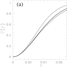
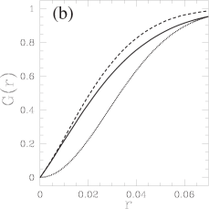
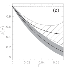
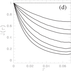
FIG. 2.: The spherical contact distribution $F(r)$ (plot (a)), the nearest neighbor distribution $G(r)$ (plot (b)) and the $J(r)$ function (plot (c)) are shown for the Gauss–Poisson process ($\varrho=200$, mean value (dashed line) and variance (shaded area) estimated from 1000 realizations), and the line–segment process ($\varrho=200$, solid line); $r$ is in units of the box length. The $J(r)$ function according to Eq. (28) (dashed dotted line) lies on top of the estimated mean. The dotted line is marking the results for a Poisson process. The sequence of solid lines in plot (d) are the $J(r)$ function for line–segment processes with $\varrho=100,150,200,300,400,500,600$, bending down successively.

In Fig. 2 the results for $F(r)$, $G(r)$, and $J(r)$, estimated from several line–segment processes, and the Gauss–Poisson process are shown; all the processes investigated had the same two–point correlation function $\xi_{2}(r)$ given in Eq. (24). The line–segment process allows for larger voids than the Gauss–Poisson process, as seen from $F_{\rm line}>F_{\rm GP}$. On small scales the $J(r)$ of the line–segment process is well approximated by the $J(r)$ for the Gauss–Poisson process. However on large scales the Gauss–Poisson process shows significantly smaller $J(r)$ function than the line–segment process. The $J(r)$ function is known analytically for several point process models [46, 48]. In any of these cases a smaller $J(r)$ is an indication for stronger (positive) interaction between the points (see also [50, 51]). Specifically for Gibbs–processes (see e.g. [15]) an attractive interaction leads to a monotonically decreasing $J(r)$ and a stronger interaction leads to smaller values of $J(r)$. Hence, the presence of higher–order correlation functions in the line–segment process gives rise to a reduced clustering strength, in the sense discussed above. Clearly, the signal of $J(r)$ also depends on the number density.

C The non–Gaussian galaxy distribution

As already mentioned, the three–dimensional distribution of galaxies cannot be modeled in terms of a Gauss–Poisson process: the constraints on the density and two–point correlation function are violated. In the following this is illustrated with a volume–limited sample of 100$h^{-1}$Mpc depth, extracted from the PSCz galaxy catalogue [52]. The volume–limited sample incorporates 2232 galaxies with galactic latitude $|b|>5^{\circ}$. A detailed description of the sample considered here may be found in [53]. Estimators for the two–point correlation function are quite abundant (see [54] and references therein). The results presented here do neither depend on the estimator, nor on the exact sample geometry, which is indeed more complicated (see [52]). For the $J(r)$–function the minus estimator is used [15, 55].

In Fig. 3 the estimated two–point correlation function is shown. The integral

$$\varrho\ \int_{{\mathbb{R}}^{3}}{\rm d}{\mathbf{y}}\ \xi_{2}(|{\mathbf{y}}|)\approx 4.4$$ (29)

is violating the constraint (19), and the corresponding Gauss-Poisson process does not exist. Indeed higher–order correlations functions have been detected by [56] using factorial moments. By thinning the galaxy distribution (i.e. randomly sub–sampling), one generates a point set with the same correlation functions $\xi_{n}$ as the observed galaxy distribution, however with a reduced number of points. Since the number density enters linearly in the constraint (19), a comparison of the thinned galaxy distribution with a Gauss–Poisson process becomes feasible. The strongly interacting galaxy distribution, as indicated by the small values of $J(r)$, shows increasingly weaker interaction (higher values of $J(r)$) for the diluted subsamples (Fig. 3).

Now consider a sample with only 20% of the actual observed galaxies, where the constraint (19) is satisfied (compare with (29)). This diluted sample is compared to a Gauss–Poisson process with the same two–point correlation function. The $\xi_{2}(r)$ determined from the simulated Gauss–Poisson process matches perfectly with the observed correlation function (Fig. 3). On small scales the $J(r)$-function of the thinned PSCz is reasonably modeled by the Gauss–Poisson process. However, on large scales the Gauss–Poisson process shows stronger interactions, whereas the thinned galaxy sample, with its higher–order correlation functions, shows weaker interactions in the sense discussed in Sect. IV B.

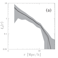
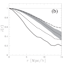
FIG. 3.: In plot (a) the observed two–point correlation function $\xi_{2}(r)$ of the volume–limited subsample with 100$h^{-1}$Mpc depth from the PSCz galaxy catalogue is shown (solid line). The dotted line and the one–$\sigma$ area are estimated from 200 realizations of a Gauss–Poisson process using the estimated two–point correlation function as an input but with only a fifth of the number of points. In plot (b) the $J(r)$ function of the same sample is shown with 100% (solid line), 50% (short dashed line), and 20% of the galaxies (long dashed line). The shaded area is the one–$\sigma$ region obtained from the Gauss–Poisson process corresponding to the galaxy sample with only 20% of the points.

V Point processes with higher–order clustering

As already mentioned, the measured two–point correlation function of the galaxy distribution together with the observed density of galaxies violates the constraints Eqs. (15) and (16). Consequently the distribution of galaxies cannot be modeled with a Gauss–Poisson process. Even more compelling, there is a clear detection of higher–order correlations in the galaxy distribution (e.g. [44, 57, 58]). Hence, one is interested in analytical tractable approximations of the cumulant expansion (7). Hierarchical closure relations have been extensively studied (see Sect. VII A). In the following a truncation of the expansion (7) beyond the Gaussian term and the $n$–point Poisson cluster processes will be used.

Such a truncation may serve as a model for the galaxy distribution in the weakly nonlinear regime. Using perturbation theory one may show that $\xi_{3}\propto(\xi_{2})^{2}$ (see [59]). For large separations $r$ the correlation function $\xi_{2}(r)$ is smaller than unity, and consequently a truncation of the expansion (7) at $n>2$ provides a viable model for the large–scale distribution of galaxies.

The general Poisson cluster process is the starting point: consider the expansion of the cluster p.g.fl. $G_{c}[h|{\mathbf{x}}]$ in terms of Janossy densities conditional on the cluster center ${\mathbf{x}}$ (see Eq. (11)):

$$G_{c}[h|{\mathbf{x}}]=J_{0}+\sum_{n=1}^{\infty}\frac{1}{n!}\int_{{\mathbb{R}}^{d}}{\rm d}{\mathbf{x}}_{1}\cdots\int_{{\mathbb{R}}^{d}}{\rm d}{\mathbf{x}}_{n}\\ j_{n}({\mathbf{x}}_{1},\ldots{\mathbf{x}}_{n}|{\mathbf{x}})\ h({\mathbf{x}}_{1})\cdots h({\mathbf{x}}_{n}).$$ (30)

Explicit expression for the Janossy densities are given below. The p.g.fl. of a Poisson cluster process is then given by

$$G[h] =\exp\Bigg{(}\int_{{\mathbb{R}}^{d}}{\rm d}{\mathbf{x}}\varrho_{c}\ (G_{c}[h|{\mathbf{x}}]-1)\Bigg{)}$$ (31)

$$=\exp\Bigg{(}\int_{{\mathbb{R}}^{d}}{\rm d}{\mathbf{x}}\varrho_{c}\ \Big{(}\sum_{n=1}^{\infty}\frac{1}{n!}\int_{{\mathbb{R}}^{d}}{\rm d}{\mathbf{x}}_{1}\cdots\int_{{\mathbb{R}}^{d}}{\rm d}{\mathbf{x}}_{n}$$ (32)

$$\qquad j_{n}({\mathbf{x}}_{1},\ldots{\mathbf{x}}_{n}|{\mathbf{x}})\ h({\mathbf{x}}_{1})\cdots h({\mathbf{x}}_{n})-1\Big{)}\Bigg{)}.$$ (33)

Here the probability $q_{0}$ of having no point in the cluster at ${\mathbf{x}}$ is assumed to be zero, i.e. $J_{0}=0$. This does not impose any additional constraints, it only leads to a redefinition of the number density of cluster centers $\varrho_{c}^{\prime}=\varrho_{c}(1+q_{0})$.

Using this more formal approach the p.g.fl. of the Gauss–Poisson process can be written in terms of the Janossy densities with $j_{n}=0$ for $n>2$:

$$\begin{split}j_{1}({\mathbf{x}}_{1}|{\mathbf{x}})&=q_{1}({\mathbf{x}})\delta^{D}({\mathbf{x}}-{\mathbf{x}}_{1}),\\ j_{2}({\mathbf{x}}_{1},{\mathbf{x}}_{2}|{\mathbf{x}})&=q_{2}({\mathbf{x}})\delta^{D}({\mathbf{x}}-{\mathbf{x}}_{1})f_{2}({\mathbf{x}}_{2}|{\mathbf{x}}_{1})\ 2!.\end{split}$$ (34)

Here $j_{1}$ ($j_{2}$) are the probability densities for the spatial distribution of one (two) points in the cluster, multiplied by the probability $q_{1}$ ($q_{2}$) that there are exactly one (two) points in the cluster at ${\mathbf{x}}$. $\delta^{D}$ is the $d$–dimensional Dirac distribution. $f_{2}({\mathbf{x}}_{2}|{\mathbf{x}}_{1})$ is the probability density of the second point ${\mathbf{x}}_{2}$ under the condition that there is a point at ${\mathbf{x}}_{1}$, normalized by $\int{\rm d}{\mathbf{x}}_{2}\ f_{2}({\mathbf{x}}_{2}|{\mathbf{x}}_{1})=1$.

The p.g.fl. (31) is invariant under changes of the order of integration, implying that one can use the $j_{n}({\mathbf{x}}_{1},\ldots{\mathbf{x}}_{n}|{\mathbf{x}})$ symmetrically defined in all coordinates (including ${\mathbf{x}}$). With the additional assumption of homogeneity and isotropy one gets $f_{2}({\mathbf{x}}_{2}|{\mathbf{x}}_{1})=f(|{\mathbf{x}}_{1}-{\mathbf{x}}_{2}|)$, as already used in Sect. III B for the construction of the Gauss–Poisson process.

A The three–point Poisson cluster process

In a three–point Poisson cluster process Eq. (31) is truncated at the third order and at most three points per cluster are allowed. Additional to Eq. (34)

$$j_{3}({\mathbf{x}}_{1},{\mathbf{x}}_{2},{\mathbf{x}}_{3}|{\mathbf{x}})=q_{3}({\mathbf{x}})\delta^{D}({\mathbf{x}}-{\mathbf{x}}_{1})f_{3}({\mathbf{x}}_{2},{\mathbf{x}}_{3}|{\mathbf{x}}_{1})\ 3!$$ (35)

appears, with the probability $q_{3}({\mathbf{x}})$ that the cluster consists out of three points, and $q_{1}+q_{2}+q_{3}=1$ with $q_{i}\geq 0$. $f_{3}({\mathbf{x}}_{2},{\mathbf{x}}_{3}|{\mathbf{x}}_{1})$ is the probability density that there are two points at ${\mathbf{x}}_{2}$, and ${\mathbf{x}}_{3}$, under the condition that one point is at ${\mathbf{x}}_{1}$, with the normalization $\int{\rm d}{\mathbf{x}}_{2}\int{\rm d}{\mathbf{x}}_{3}\ f_{3}({\mathbf{x}}_{2},{\mathbf{x}}_{3}|{\mathbf{x}}_{1})=1$. Inserting these definitions one obtains

$$\log G[h]=\int_{{\mathbb{R}}^{d}}{\rm d}{\mathbf{x}}_{1}\ \varrho_{p}q_{1}({\mathbf{x}}_{1})\ (h({\mathbf{x}}_{1})-1)+\\ +\int_{{\mathbb{R}}^{d}}{\rm d}{\mathbf{x}}_{1}\ \varrho_{p}\int_{{\mathbb{R}}^{d}}{\rm d}{\mathbf{x}}_{2}\ q_{2}({\mathbf{x}}_{1})f_{2}({\mathbf{x}}_{2}|{\mathbf{x}}_{1})\ (h({\mathbf{x}}_{1})h({\mathbf{x}}_{2})-1)+\\ +\int_{{\mathbb{R}}^{d}}{\rm d}{\mathbf{x}}_{1}\ \varrho_{p}\int_{{\mathbb{R}}^{d}}{\rm d}{\mathbf{x}}_{2}\int_{{\mathbb{R}}^{d}}{\rm d}{\mathbf{x}}_{3}\ q_{3}({\mathbf{x}}_{1})f_{3}({\mathbf{x}}_{2},{\mathbf{x}}_{3}|{\mathbf{x}}_{1})\times\\ \times\Big{(}h({\mathbf{x}}_{1})h({\mathbf{x}}_{2})h({\mathbf{x}}_{3})-1\Big{)}.$$ (36)

As already mentioned, $f_{3}({\mathbf{x}}_{2},{\mathbf{x}}_{3}|{\mathbf{x}}_{1})$ can be assumed to be symmetric in its three arguments. Slightly abusing notation, let $f_{2}({\mathbf{x}}_{1},{\mathbf{x}}_{2})$ and $f_{3}({\mathbf{x}}_{1},{\mathbf{x}}_{2},{\mathbf{x}}_{3})$ be the symmetrically defined densities corresponding to $f_{2}({\mathbf{x}}_{2}|{\mathbf{x}}_{1})$ and $f_{3}({\mathbf{x}}_{2},{\mathbf{x}}_{3}|{\mathbf{x}}_{1})$, and define

$$f_{2}^{(3)}({\mathbf{x}}_{1},{\mathbf{x}}_{2})=\int_{{\mathbb{R}}^{d}}{\rm d}{\mathbf{x}}_{3}\ f_{3}({\mathbf{x}}_{1},{\mathbf{x}}_{2},{\mathbf{x}}_{3}).$$ (37)

Replacing $h$ by $h+1$ and rearranging the terms the factorial cumulant expansion of the three–point cluster process reads

$$\log G[h+1]=\int_{{\mathbb{R}}^{d}}{\rm d}{\mathbf{x}}_{1}\ h({\mathbf{x}}_{1})\ \varrho_{p}\big{(}1+q_{2}({\mathbf{x}}_{1})+2q_{3}({\mathbf{x}}_{1})\big{)}+\\ \begin{aligned} +&\int_{{\mathbb{R}}^{d}}{\rm d}{\mathbf{x}}_{1}\int_{{\mathbb{R}}^{d}}{\rm d}{\mathbf{x}}_{2}\ h({\mathbf{x}}_{1})h({\mathbf{x}}_{2})\times\\ &\quad\times\varrho_{p}\Big{(}q_{2}({\mathbf{x}}_{1})f_{2}({\mathbf{x}}_{1},{\mathbf{x}}_{2})+3q_{3}({\mathbf{x}}_{1})f_{2}^{(3)}({\mathbf{x}}_{1},{\mathbf{x}}_{2})\Big{)}+\\ +&\int_{{\mathbb{R}}^{d}}{\rm d}{\mathbf{x}}_{1}\int_{{\mathbb{R}}^{d}}{\rm d}{\mathbf{x}}_{2}\int_{{\mathbb{R}}^{d}}{\rm d}{\mathbf{x}}_{3}\ h({\mathbf{x}}_{1})h({\mathbf{x}}_{2})h({\mathbf{x}}_{3})\times\\ &\quad\times\varrho_{p}q_{3}({\mathbf{x}}_{1})f_{3}({\mathbf{x}}_{1},{\mathbf{x}}_{2},{\mathbf{x}}_{3}).\end{aligned}$$ (38)

Comparing Eq. (38) with the expansion (7) one arrives at

$$\varrho =(q_{1}+2q_{2}+3q_{3})\varrho_{p}=(1+q_{2}+2q_{3})\varrho_{p}$$ (39)

$$\xi_{2}({\mathbf{x}}_{1},{\mathbf{x}}_{2}) =\frac{2!}{(1+q_{2}+2q_{3})^{2}\varrho_{p}}\times$$ (40)

$$\quad\times\Big{(}q_{2}f_{2}({\mathbf{x}}_{1},{\mathbf{x}}_{2})+3q_{3}f_{2}^{(3)}({\mathbf{x}}_{1},{\mathbf{x}}_{2})\Big{)}$$ (41)

$$\xi_{3}({\mathbf{x}}_{1},{\mathbf{x}}_{2},{\mathbf{x}}_{3}) =\frac{3!}{(1+q_{2}+2q_{3})^{3}\varrho_{p}^{2}}\ q_{3}f_{3}({\mathbf{x}}_{1},{\mathbf{x}}_{2},{\mathbf{x}}_{3}),$$ (42)

and the correlation functions $\xi_{n}$ equal zero for $n\geq 4$. The simulation procedure for the three–point Poisson cluster process is described in Appendix B 2.

B Constraints on $\varrho$, $\xi_{2}$ and $\xi_{3}$

By the definition of the three–point Poisson cluster process, the probability densities $f_{2}\geq 0$, $f_{3}\geq 0$, and $f_{2}^{(3)}\geq 0$ and consequently $\xi_{2}(r)\geq 0$ for all $r$, as well as $\xi_{3}\geq 0$. This is a generic feature of Poisson cluster processes.

The Gauss–Poisson process, defined through the truncation of the cumulant expansion after the second term, is equivalent to the two–point Poisson cluster process (see Sect. III B). Unfortunately, this equivalence does not hold for the higher $n$–point processes anymore. The general three–point process is defined as point process with a factorial cumulant expansion truncated after the third term. Proceeding similar to Sect. III A, necessary conditions for the existence of such a point process can be derived (compare with Eq. (14)):

$$0\leq\varrho|A_{l}|+\sum_{i=1}^{k}\varrho^{2}|A_{l}||A_{i}|\overline{\xi}_{2}(A_{l},A_{i})(z_{i}-1)+\\ +\sum_{i=1}^{k}\sum_{j=1}^{k}\frac{\varrho^{3}}{2}|A_{l}||A_{i}||A_{j}|\overline{\xi}_{3}(A_{l},A_{i},A_{j})(z_{i}-1)(z_{j}-1),$$ (43)

with the volume–averaged correlation functions

$$\overline{\xi}_{n}(A_{1},\ldots,A_{n})=\frac{1}{|A_{1}|\cdots|A_{n}|}\times\\ \times\int_{A_{1}}{\rm d}{\mathbf{x}}_{1}\cdots\int_{A_{n}}{\rm d}{\mathbf{x}}_{n}\ \xi_{n}({\mathbf{x}}_{1},\ldots,{\mathbf{x}}_{n}),$$ (44)

and for consistency $\overline{\xi}_{1}(A)=1$. Again, for $z_{i}=1$ one obtains $\varrho\geq 0$. The non–trivial constraints read:

$$1\geq \ \varrho|A_{s}|\overline{\xi}_{2}(A_{l},A_{s})-\varrho^{2}|A_{s}|^{2}\overline{\xi}_{3}(A_{l},A_{s},A_{s}),$$ (45)

$$0\leq \ \overline{\xi}_{3}(A_{l},A_{s},A_{s}),$$ (46)

$$1\geq \ \varrho|A_{s}|\overline{\xi}_{2}(A_{l},A_{s})+\varrho|A_{r}|\overline{\xi}_{2}(A_{l},A_{r})-$$ (47)

$$\ -\frac{\varrho^{2}}{2}|A_{s}|^{2}\overline{\xi}_{3}(A_{l},A_{s},A_{s})-\frac{\varrho^{2}}{2}|A_{r}|^{2}\overline{\xi}_{3}(A_{l},A_{r},A_{r})-$$ (48)

$$\ -\varrho^{2}|A_{s}||A_{r}|\overline{\xi}_{3}(A_{l},A_{s},A_{r}).$$ (49)

Eq. (45) can be derived by setting $z_{s}=0$ and $z_{i}=1$ for all $i\neq s$, Eq. (46) follows from $z_{s}\rightarrow\infty$ and $z_{i}=1$ for all $i\neq s$. Using $z_{r},z_{s}\rightarrow\infty$ does not lead to new constraints. With $z_{r}=0=z_{s}$, $r\neq s$, and $z_{i}=1$ for all $i\neq r,s$ one obtains Eq. (47). No additional constraint arises by setting $z=2$.

Eq. (46) implies $\xi_{3}\geq 0$. Eq. (45) and Eq. (47) are the extension of the constraint (17). The terms proportional to $\overline{\xi}_{3}$ can balance the terms with $\overline{\xi}_{2}$, and a clustering point processes with a number density higher than in a Gauss–Poisson process is possible. Moreover, $\xi_{2}$ is not constrained to positive values anymore. Hence, already by including three–point correlations, a point process model with a two–point correlation function $\xi_{2}$ having a zero crossing becomes admissible. This answers affirmatively the question by [60], whether there exists a general three–point cluster processes with a negative second moment. However, in the three–point Poisson cluster process discussed in the preceding section a $\xi_{2}\geq 0$ is required illustrating that the three–point Poisson cluster processes form only a subset of all possible three–point processes.

C The $n$–point Poisson cluster process

It is now clear how to construct the $n$–point Poisson cluster process. Let $q_{m}$ be the probability of having $m$ points per cluster with $\sum_{m=1}^{n}q_{m}=1$.

$$j_{n}({\mathbf{x}}_{1},\ldots,{\mathbf{x}}_{n}|{\mathbf{x}})=q_{n}({\mathbf{x}})\delta^{D}({\mathbf{x}}-{\mathbf{x}}_{1})f_{n}({\mathbf{x}}_{2},\ldots,{\mathbf{x}}_{n}|{\mathbf{x}}_{1})\ n!,$$ (50)

determines the distribution of the $n$ points inside the cluster ($f_{1}=1$). As above the $f_{n}$ are assumed to be symmetric in all their arguments, and for $n>m$

$$f_{m}^{(n)}({\mathbf{x}}_{1},\ldots,{\mathbf{x}}_{m})=\int_{{\mathbb{R}}^{d}}{\rm d}{\mathbf{x}}_{m+1}\cdots\int_{{\mathbb{R}}^{d}}{\rm d}{\mathbf{x}}_{n}\\ f_{n}({\mathbf{x}}_{1},\ldots,{\mathbf{x}}_{m},{\mathbf{x}}_{m+1},\ldots,{\mathbf{x}}_{n}),$$ (51)

and $f_{m}=f_{m}^{(m)}$. Inserting Eq. (50) into Eq. (31) and after some algebraic manipulations one can compare term by term with the factorial cumulant expansion (7) of the p.g.fl.:

$$\varrho =\varrho_{p}\sum_{m=1}^{n}mq_{m}$$ (52)

$$\xi_{k}({\mathbf{x}}_{1},\ldots,{\mathbf{x}}_{k}) =\frac{k!\varrho_{p}}{\varrho^{k}}\sum_{m=k}^{n}\binom{m}{k}q_{m}f_{k}^{(m)}({\mathbf{x}}_{1},\ldots,{\mathbf{x}}_{k}),$$ (53)

with $k\leq n$, and $\xi_{k}=0$ for $k>n$. The statistical properties of this $n$–point Poisson cluster process are now completely specified by the correlation functions $\xi_{k}$ with $k\leq n$ and the mean density $\varrho$. Eqs. (52) and the normalization of the $f_{m}$ can be used to determine the $f_{m}$ as well as $\varrho_{p}$ and $q_{m}$ from given correlation functions $\xi_{n}$ and the number density $\varrho$. A simulation algorithm similar to the one described in Appendix B 2 can be constructed.

D The general $n$–point process

The general $n$–point process is defined as the point process resulting from the factorial cumulant expansion truncated after the $n$th term. Proceeding similarly to Sect. III A one arrives at the constraint equations

$$0\geq\varrho|A_{l}|+\varrho^{2}\sum_{i=1}^{k}|A_{l}||A_{i}|\overline{\xi}_{2}(A_{l},A_{i})(z_{i}-1)+\ldots+\\ +\frac{\varrho^{n}n}{n!}\sum_{i_{1},\ldots,i_{n-1}=1}^{k}|A_{l}||A_{i_{1}}|\cdots|A_{i_{n-1}}|\times\\ \times\overline{\xi}_{n}(A_{l},A_{i_{1}},\ldots,A_{i_{n-1}})(z_{i_{1}}-1)\cdots(z_{i_{n-1}}-1).$$ (54)

It is now possible to compute the constraints for the $n$–point process, in close analogy to the three–point process in Sect. V B. [60] gave necessary and sufficient conditions for the existence of a generalized Hermite distribution (closely related to this $n$–point process). They discuss the constraints for a slightly different expansion of the p.g.f. Unfortunately, the transformation of their expansion to the expansion in terms of correlation functions is as tedious as the direct calculation of the constraints.

VI Random fields vs. point processes

A random field $u({\mathbf{x}})$ is in the simplest case a real–valued function on ${\mathbb{R}}^{d}$ [31]. In cosmology the initial mass–density field is often modeled as a Gaussian random field (see e.g. [2, 61]). The nonlinear evolution of the density field unavoidably introduces higher–order correlations. A random field $u(x)$ is stochastically characterized by its characteristic functional (e.g. [62])

$$\Phi^{u}[v]={\mathbb{E}}^{u}\Bigg{[}\exp\Bigg{(}i\int_{{\mathbb{R}}^{d}}{\rm d}{\mathbf{x}}\ v({\mathbf{x}})u({\mathbf{x}})\Bigg{)}\Bigg{]},$$ (55)

where ${\mathbb{E}}^{u}$ denotes the expectation value over realizations of the random field $u$. In close analogy to the expansion (A5) of the characteristic function of a random variable in terms of cumulants, one obtains the expansion of the characteristic functional

$$\ln\Phi^{u}[v]=\sum_{n=1}^{\infty}\frac{i^{n}}{n!}\int_{{\mathbb{R}}^{d}}{\rm d}{\mathbf{x}}_{1}\cdots\int_{{\mathbb{R}}^{d}}{\rm d}{\mathbf{x}}_{n}\\ c_{n}^{u}({\mathbf{x}}_{1},\ldots,{\mathbf{x}}_{n})\ v({\mathbf{x}}_{1})\cdots v({\mathbf{x}}_{n})$$ (56)

in terms of $n$-point cumulants $c_{n}^{u}({\mathbf{x}}_{1},\ldots,{\mathbf{x}}_{n})$. Here $c_{1}^{u}({\mathbf{x}})={\mathbb{E}}^{u}[u({\mathbf{x}})]=\overline{u}$ is the mean value. The correlation function of the field is

$$\xi_{2}^{u}({\mathbf{x}}_{1},{\mathbf{x}}_{2})=\frac{c_{2}^{u}({\mathbf{x}}_{1},{\mathbf{x}}_{2})}{\overline{u}^{2}}=\frac{{\mathbb{E}}^{u}[u({\mathbf{x}}_{1})u({\mathbf{x}}_{2})]}{\overline{u}^{2}}-1,$$ (57)

and similar for higher–order correlation functions (see e.g. [62, 63]). The well known characteristic functional of the Gaussian random field reads

$$\ln\Phi^{u}[v]=i\int_{{\mathbb{R}}^{d}}{\rm d}{\mathbf{x}}_{1}\ \overline{u}v({\mathbf{x}}_{1})-\\ -\frac{1}{2}\int_{{\mathbb{R}}^{d}}{\rm d}{\mathbf{x}}_{1}\int_{{\mathbb{R}}^{d}}{\rm d}{\mathbf{x}}_{2}\ c_{2}^{u}({\mathbf{x}}_{1},{\mathbf{x}}_{2})\ v({\mathbf{x}}_{1})v({\mathbf{x}}_{2}),$$ (58)

with the covariance function $c_{2}^{u}({\mathbf{x}}_{1},{\mathbf{x}}_{2})$.

The characteristic functional of a point process is defined by

$$\Phi[h]={\mathbb{E}}\left[\exp\left(i\int_{{\mathbb{R}}^{d}}N({\rm d}{\mathbf{x}})h({\mathbf{x}})\right)\right],$$ (59)

and the relation to the p.g.fl. is $\Phi[h]=G[{\rm e}^{ih}]$. An expansion into cumulants $c_{k}({\mathbf{x}}_{1},...,{\mathbf{x}}_{k})$ is also possible:

$$\log\Phi[h]=\sum_{k=1}^{\infty}\frac{i^{k}}{k!}\int_{{\mathbb{R}}^{d}}{\rm d}{\mathbf{x}}_{1}\cdots\int_{{\mathbb{R}}^{d}}{\rm d}{\mathbf{x}}_{k}\\ c_{k}({\mathbf{x}}_{1},\ldots,{\mathbf{x}}_{k})\ h({\mathbf{x}}_{1})\cdots h({\mathbf{x}}_{k}).$$ (60)

The cumulants $c_{k}(\cdot)$ should not be confused with the factorial cumulants $c_{[k]}(\cdot)$.

A A theorem of Marcinkiewicz

A theorem of Marcinkiewicz [64] states that if the characteristic function $\varphi(s)$ of a random variable (see Appendix A) is the exponential of a polynomial with finite degree larger than two, then the positive definiteness of the probability distribution is violated (see e.g. [65, 66, 67]). The generalized Marcinkiewicz theorem for characteristic functionals [68, 69] tells us that this expansion has to be either infinite or a polynomial in $h({\mathbf{x}})$ (or $v({\mathbf{x}})$) of degree less than or equal to two. This directly applies to the expansion of the characteristic functionals of a random field $\Phi^{u}[v]$ and a point process $\Phi[h]$ in terms of cumulants.

However, for a point process one can see that the expansion of the p.g.fl. in terms of factorial cumulants $c_{[k]}(\cdot)$ (or correlation functions $\xi_{k}(\cdot)$) allows a truncation at a finite $k>2$. As long as constraints on the density and the correlation functions are fulfilled, the point process is well defined. Although the p.g.fl. was used mainly in the context of discrete events, it seems worthwhile to consider the characterizations of random fields with factorial cumulants.

Another systematic expansion is provided by the Edgeworth series. It was successfully applied in cosmology to quantify the one point probability distribution function for the smoothed density field on large scales [70]. Recently, [71] showed how to use the truncated Edgeworth series to generate realizations of non–Gaussian random fields with predefined correlation properties. The truncated Edgeworth series also violates the positive definiteness of the probability distribution, but [71] restore the positivity, reintroducing higher correlations, leading to a “leaking” into higher correlations.

The cumulants $c_{k}$ and the factorial cumulants $c_{[k]}$ of a random variable are related by $c_{k}=\sum_{l=1}^{k}s_{2}(k,l)\ c_{[l]}$ (see Eq. (A16)). Looking at the Poisson cluster processes discussed in the preceding sections, one observes that such a relation must not hold between the cumulants and the factorial cumulants of a point process. As an example consider the three–point Poisson cluster process with $c_{[n]}(\cdot)=0$ for all $n>3$. A finite $c_{[3]}(\cdot)$ leads to non–zero $c_{n}(\cdot)$ for all $n$ (see Appendix C for details.)

B The Poisson model

In cosmology the point distribution is often related to the mass density field assuming the “Poisson model”. The value of the mass density field is assumed to be proportional to the local number density, and the point distribution is constructed by “Poisson sampling” the correlated mass density field. If the mass density field is itself a realization of a random field, the resulting point process is called a Cox process, or doubly stochastic process. Within this model one may show that the cumulants $c_{n}^{u}$ of the density field are proportional to the factorial cumulants $c_{[n]}$ of the point distribution [72, 26]: $c_{[n]}=c_{n}^{u}\ \rho^{2}/\overline{u}^{2}$. It is important to notice that this relates the characteristic functional of the random field $\Phi^{u}[v]$ with the p.g.fl of the point process $G[h]$. For the correlation functions one obtains

$$\xi_{n}({\mathbf{x}}_{1},\ldots,{\mathbf{x}}_{n})=\xi_{n}^{u}({\mathbf{x}}_{1},\ldots,{\mathbf{x}}_{n}).$$ (61)

Hence, this model allows the direct comparison of predictions from analytical calculations with the observed correlation functions in the galaxy distribution.

Clearly the question arises, what is wrong with the simple picture that one starts with a Gaussian random field and “Poisson sample” it to obtain the desired point distribution. The answer is that a Gaussian random field is an approximate model for a mass density field only if the fluctuations are significantly smaller than the mean mass density. Otherwise negative mass densities (i.e. negative “probabilities” for the Poisson sampling) would occur. Only in the limit of vanishing fluctuations a Poisson sampled Gaussian random field becomes a permissible model. However, in this limit one is left with a pure Poisson process.

VII Models for strongly correlated systems

In the Sects. III and V several types of point processes were discussed, all featuring a truncated factorial cumulant expansion. As argued at the beginning of Sect. V, such a truncation is feasible for the matter distribution in the Universe, as long as $\xi_{2}(r)<1$, i.e. for points with large separations. Mainly two approaches have been followed to model the galaxy distribution also on small scales with $\xi_{2}(r)\gg 1$. The hierarchical models are briefly discussed in the next section and in Sect. VII B an extension of the halo–model is presented.

A Hierarchical models

In cosmology one often starts with a scale–invariant correlation function $\xi_{2}(r)\propto{r}^{-\gamma}$ and assumes some closure relations for the $\xi_{n}$. Especially the hierarchical ansatz $\xi_{n}=Q_{n}\sum_{\text{trees}}\prod^{n-1}\xi_{2}$ was extensively studied (e.g. [72, 73, 74, 8, 75, 9], and more recent [76, 77]). [8] discuss conditions for the coefficients $Q_{n}$ such that the expansion of the p.g.f.’s in terms of the count–in–cells converges. In this case the count–in–cells uniquely determine the point process. As illustrated in Sect. VIII with the log–normal distribution, a non–converging expansion does not necessarily imply that the stochastic model is not well–defined. It only implies that such a point process model is not completely specified by its correlation functions. For critical systems similar expansion in terms of correlation functions are typically divergent (see e.g. [78], chapt. 41).

As another closure relation Kirkwood [79] employed the following approximation

$$\varrho_{3}({\mathbf{x}}_{1},{\mathbf{x}}_{2},{\mathbf{x}}_{3})=\\ \varrho^{3}(1+\xi_{2}({\mathbf{x}}_{1},{\mathbf{x}}_{2}))(1+\xi_{2}({\mathbf{x}}_{2},{\mathbf{x}}_{3}))(1+\xi_{2}({\mathbf{x}}_{3},{\mathbf{x}}_{1}))$$ (62)

to calculate thermodynamic properties of fluids using the BBGKY hierarchy. This closure relation is exact for the log–normal distribution (e.g. [80]). Empirically however one finds that this ansatz is disfavored as a model for the galaxy distribution [81].

B The generalized halo model

In Sect. V several types of Poisson cluster processes were constructed by starting with Poisson distributed centers and attaching a secondary point process, the cluster, to each point. One can generalize this procedure by considering cluster centers given by already correlated points. One possibility, is to iterate the construction principle of the simple Poisson cluster process leading to the $m$–th order Neyman–Scott processes [5]. If one is only interested in the first few correlation functions, the full specification of the point process is not necessary. Within the halo model (see e.g. [21, 17, 82, 18, 19, 20]) it is specifically easy to calculate the correlation functions. The difference to the Poisson cluster processes discussed previously is that the cluster centers now may be correlated themselves. The major physical assumption entering is that the properties of the clusters (halos) are independent from the positions and correlations of the cluster centers.

Consider a point process for the cluster centers, the parents, specified by the p.g.fl. $G_{p}[h]$. Independent from the distribution of the centers, a cluster with a p.g.fl. $G_{c}[h|{\mathbf{y}}]$ is attached to each center ${\mathbf{y}}$. Then the p.g.fl. of this cluster process is given by the “folding” of the two p.g.fl.’s [26]:

$$G[h]=G_{p}\big{[}G_{c}[h|\cdot]\big{]}.$$ (63)

Using the expansion (7), these p.g.fl.’s are given by

$$\log G_{p}[h+1] =\sum_{m=1}^{\infty}\frac{\varrho_{p}^{m}}{m!}\int_{{\mathbb{R}}^{d}}{\rm d}{\mathbf{y}}_{1}\cdots\int_{{\mathbb{R}}^{d}}{\rm d}{\mathbf{y}}_{m}$$ (64)

$$\quad\xi_{m}^{(p)}({\mathbf{y}}_{1},\ldots,{\mathbf{y}}_{m})\ h({\mathbf{y}}_{1})\cdots h({\mathbf{y}}_{m}),$$ (65)

$$\log G_{c}[h+1|{\mathbf{y}}] =\sum_{n=1}^{\infty}\frac{1}{n!}\int_{{\mathbb{R}}^{d}}{\rm d}{\mathbf{x}}_{1}\cdots\int_{{\mathbb{R}}^{d}}{\rm d}{\mathbf{x}}_{n}$$ (66)

$$\quad c_{[n]}({\mathbf{x}}_{1},\ldots,{\mathbf{x}}_{n}|{\mathbf{y}})\ h({\mathbf{x}}_{1})\cdots h({\mathbf{x}}_{n}),$$ (67)

where $\varrho_{p}$ is the number density and the $\xi_{n}^{(p)}$ are the correlation functions of the parent process. The $c_{[n]}(\ldots|{\mathbf{y}})$ are the factorial cumulants specifying the point distribution in a cluster, conditional on the cluster center ${\mathbf{y}}$. $c_{[1]}({\mathbf{x}}|{\mathbf{y}})$ is the halo profile, with the mean number of points per halo $\mu=\int{\rm d}{\mathbf{x}}\ c_{[1]}({\mathbf{x}}|{\mathbf{y}})$. The $c_{[n]}$, $n\geq 2$ quantify the halo substructure. A halo without substructure is an inhomogeneous Poisson process, and completely characterized by $c_{[1]}({\mathbf{x}}|{\mathbf{y}})$ and $c_{[n]}=0$, $n\geq 2$. Combining Eqs. (63) and (64)

$$\log G[h+1]=\sum_{m=1}^{\infty}\frac{\varrho_{p}^{m}}{m!}\int_{{\mathbb{R}}^{d}}{\rm d}{\mathbf{y}}_{1}\cdots\int_{{\mathbb{R}}^{d}}{\rm d}{\mathbf{y}}_{m}\\ \xi_{m}^{(p)}({\mathbf{y}}_{1},\ldots,{\mathbf{y}}_{m})\ \prod_{i=1}^{m}\big{(}G_{c}[h+1|{\mathbf{y}}_{i}]-1\big{)},$$ (68)

one immediately recovers the p.g.fl. of the Poisson cluster process Eq. (21) by setting $\xi_{m}^{(p)}=0$ for $m\geq 2$ ($\xi_{1}^{(p)}=1$).

C $\xi_{2}$ and $\xi_{3}$ in the generalized halo model

In the standard halo model the clusters are simply modeled by an inhomogeneous Poisson process, whereas the centers are given by a correlated point process, typically determined from the evolved density distribution. Based on these assumptions one can calculate the correlation functions $\xi_{n}$ for the halo model [21, 17]. Both theoretical models as well as observations suggest that dark matter caustics lead to substructure inside halos [83]. Also recent high–resolution $N$–body simulations suggest that 15%–40% of the simulated halos show a significant amount of substructure (see [84] and references therein). To generalize the halo model, the correlations inside the halo are taken into account.

Consider the expansion of $G_{c}[h|{\mathbf{y}}_{i}]-1$ in $h$:

$$G_{c}[h|{\mathbf{y}}_{i}]-1=\int_{{\mathbb{R}}^{d}}{\rm d}{\mathbf{x}}_{1}\ h({\mathbf{x}}_{1})\ c_{[1]}({\mathbf{x}}_{1}|{\mathbf{y}}_{i})+$$ (69)

$$+\frac{1}{2!}\int_{{\mathbb{R}}^{d}}{\rm d}{\mathbf{x}}_{1}\int_{{\mathbb{R}}^{d}}{\rm d}{\mathbf{x}}_{2}\ h({\mathbf{x}}_{1})h({\mathbf{x}}_{2})\times$$ (70)

$$\qquad\times\Big{(}c_{[1]}({\mathbf{x}}_{1}|{\mathbf{y}}_{i})c_{[1]}({\mathbf{x}}_{2}|{\mathbf{y}}_{i})+c_{[2]}({\mathbf{x}}_{1},{\mathbf{x}}_{2}|{\mathbf{y}}_{i})\Big{)}+$$ (71)

$$+\frac{1}{3!}\int_{{\mathbb{R}}^{d}}{\rm d}{\mathbf{x}}_{1}\int_{{\mathbb{R}}^{d}}{\rm d}{\mathbf{x}}_{2}\int_{{\mathbb{R}}^{d}}{\rm d}{\mathbf{x}}_{3}\ h({\mathbf{x}}_{1})h({\mathbf{x}}_{2})h({\mathbf{x}}_{3})\times$$ (72)

$$\qquad\times\Big{(}c_{[1]}({\mathbf{x}}_{1}|{\mathbf{y}}_{i})c_{[1]}({\mathbf{x}}_{2}|{\mathbf{y}}_{i})c_{[1]}({\mathbf{x}}_{3}|{\mathbf{y}}_{i})+$$ (73)

$$\qquad+3\ c_{[2]}({\mathbf{x}}_{1},{\mathbf{x}}_{2}|{\mathbf{y}}_{i})c_{[1]}({\mathbf{x}}_{3}|{\mathbf{y}}_{i})+c_{3}({\mathbf{x}}_{1},{\mathbf{x}}_{2},{\mathbf{x}}_{3}|{\mathbf{y}}_{i})\Big{)}+$$ (74)

$$+O[h^{4}].$$ (75)

After inserting this expansion into Eq. (68) and collecting terms proportional to powers of $\varrho{}h(\cdot)$, with the mean number density $\varrho=\varrho_{p}\mu$, one can directly compare with the expansion (7) and read off the correlation functions:

$$\xi_{2}({\mathbf{x}}_{1},{\mathbf{x}}_{2})=\\ =\frac{1}{\varrho_{p}\mu^{2}}\int_{{\mathbb{R}}^{d}}{\rm d}{\mathbf{y}}_{1}\Big{(}c_{[1]}({\mathbf{x}}_{1}|{\mathbf{y}}_{1})c_{[1]}({\mathbf{x}}_{2}|{\mathbf{y}}_{1})+c_{[2]}({\mathbf{x}}_{1},{\mathbf{x}}_{2}|{\mathbf{y}}_{1})\Big{)}+\\ +\frac{1}{\mu^{2}}\int_{{\mathbb{R}}^{d}}{\rm d}{\mathbf{y}}_{1}\int_{{\mathbb{R}}^{d}}{\rm d}{\mathbf{y}}_{2}\ \xi_{2}^{(p)}({\mathbf{y}}_{1},{\mathbf{y}}_{2})\ c_{[1]}({\mathbf{x}}_{1}|{\mathbf{y}}_{1})c_{[1]}({\mathbf{x}}_{2}|{\mathbf{y}}_{2}),$$ (76)

$$\xi_{3}({\mathbf{x}}_{1},{\mathbf{x}}_{2},{\mathbf{x}}_{3})=$$ (77)

$$= \frac{1}{\varrho_{p}^{2}\mu^{3}}\int_{{\mathbb{R}}^{d}}{\rm d}{\mathbf{y}}_{1}\Big{(}c_{[1]}({\mathbf{x}}_{1}|{\mathbf{y}}_{1})c_{[1]}({\mathbf{x}}_{2}|{\mathbf{y}}_{1})c_{[1]}({\mathbf{x}}_{3}|{\mathbf{y}}_{1})+$$ (78)

$$\qquad+3c_{[1]}({\mathbf{x}}_{1}|{\mathbf{y}}_{1})c_{[2]}({\mathbf{x}}_{2},{\mathbf{x}}_{3}|{\mathbf{y}}_{1})+c_{3}({\mathbf{x}}_{1},{\mathbf{x}}_{2},{\mathbf{x}}_{3}|{\mathbf{y}}_{1})\Big{)}+$$ (79)

$$+\frac{3}{\varrho_{p}\mu^{3}}\int_{{\mathbb{R}}^{d}}{\rm d}{\mathbf{y}}_{1}\int_{{\mathbb{R}}^{d}}{\rm d}{\mathbf{y}}_{2}\ \xi_{2}^{(p)}({\mathbf{y}}_{1},{\mathbf{y}}_{2})\times$$ (80)

$$\qquad\times\Big{(}c_{[1]}({\mathbf{x}}_{1}|{\mathbf{y}}_{1})c_{[1]}({\mathbf{x}}_{2}|{\mathbf{y}}_{2})c_{[1]}({\mathbf{x}}_{3}|{\mathbf{y}}_{2})+$$ (81)

$$\qquad\qquad+c_{[1]}({\mathbf{x}}_{1}|{\mathbf{y}}_{1})c_{[2]}({\mathbf{x}}_{2},{\mathbf{x}}_{3}|{\mathbf{y}}_{2})\Big{)}+$$ (82)

$$+\frac{1}{\mu^{3}}\int_{{\mathbb{R}}^{d}}{\rm d}{\mathbf{y}}_{1}\int_{{\mathbb{R}}^{d}}{\rm d}{\mathbf{y}}_{2}\int_{{\mathbb{R}}^{d}}{\rm d}{\mathbf{y}}_{3}\ \xi_{3}^{(p)}({\mathbf{y}}_{1},{\mathbf{y}}_{2},{\mathbf{y}}_{3})\times$$ (83)

$$\qquad\qquad\times c_{[1]}({\mathbf{x}}_{1}|{\mathbf{y}}_{1})c_{[1]}({\mathbf{x}}_{2}|{\mathbf{y}}_{2})c_{[1]}({\mathbf{x}}_{3}|{\mathbf{y}}_{3}).$$ (84)

Similarly the higher $n$–point correlation functions can be calculated.

In current calculations of the two– and three–point functions for the halo model [17, 82] the galaxies inside the halos are modeled as an inhomogeneous (finite) Poisson process. The halo profile $c_{[1]}({\mathbf{x}}|{\mathbf{y}})$ is conditional on the cluster center ${\mathbf{y}}$, but no substructure inside halos is present, i.e. $c_{[n]}=0$ for $n\geq 2$. In this case the above expressions simplify to the result of [21].

The simulation of such a point distribution can be carried out in a multi–step approach similar to the simulation of the Gauss–Poisson process (Appendix B 1). First generate the correlated cluster centers, e.g. by using a Gauss–Poisson process or a low–resolution simulation, and then attach a secondary point process either modeled as an inhomogeneous Poisson or $n$–point Poisson cluster process.

D Halo substructure

The following discussion shall serve mainly as an illustration of how to incorporate halo substructure in calculations of the correlation function. To keep things simple the following assumptions are made: the halo profile $c_{[1]}({\mathbf{x}}|{\mathbf{y}})=c_{[1]}(|{\mathbf{x}}-{\mathbf{y}}|)$ is independent from the mass of the halo, and $c_{[2]}({\mathbf{x}}_{1},{\mathbf{x}}_{2}|{\mathbf{y}})$ factors into $c_{[1]}({\mathbf{x}}_{1}|{\mathbf{y}})c_{[1]}({\mathbf{x}}_{2}|{\mathbf{y}})\gamma(|{\mathbf{x}}_{1}-{\mathbf{x}}_{2}|)$, as expected for locally isotropic substructures. Let $P^{(p)}(k)=\int\frac{{\rm d}{\mathbf{x}}}{(2\pi)^{3}}\xi_{2}^{(p)}(|{\mathbf{x}}|){\rm e}^{-i{\mathbf{k}}\cdot{\mathbf{x}}}$ be the power spectrum of the spatial distribution of the halo centers, and let $\widetilde{c}_{[1]}(k)$ and $\widetilde{\gamma}(k)$ be the Fourier transform of $c_{[1]}$ and $\gamma$ respectively. The power spectrum of the galaxy distribution in the generalized halo model is then

$$P(k)=\frac{(2\pi)^{3}}{\varrho_{p}\mu^{2}}|\widetilde{c}_{1}(k)|^{2}+\frac{(2\pi)^{6}}{\mu^{2}}|\widetilde{c}_{[1]}(k)|^{2}P^{(p)}(k)+\\ +\frac{(2\pi)^{3}}{\varrho_{p}\mu^{2}}\int{\rm d}{\mathbf{k}}^{\prime}\ |\widetilde{c}_{[1]}(k^{\prime})|^{2}\widetilde{\gamma}(|{\mathbf{k}}-{\mathbf{k}}^{\prime}|).$$ (85)

This first two terms are the result of [21], the additional term accounts for halo–substructure and involves a folding of $\widetilde{c}_{[1]}$ with $\widetilde{\gamma}$ in Fourier–space. Similar expressions can be derived from Eq. (77) for the bispectrum. Quantitative predictions for the galaxy distribution, similar to the investigations by [17], will be the topic of future work.

VIII Some open problems

Our investigations rested on the assumption that the correlation functions exist and that the expansions of the p.g.fl. converge. In this case the p.g.fl., and consequently the point process, is determined completely by the correlation functions. The first assumption, the existence of the correlation functions (the factorial cumulants), does not impose dramatic restrictions for the models. In classical systems the mean number of points ${\mathbb{E}}[N]$ as well as the factorial moments ${\mathbb{E}}[N(N-1)\cdots(N-n+1)]$ should be finite in any bounded domain. For the $n$–point Poisson cluster processes, discussed in the preceding sections, at maximum $n$ points reside in a cluster, which are themselves distributed according to a Poisson process with constant number density. Clearly in such a simple situation both assumptions are satisfied. However, even for physically well motivated models, the convergence of the expansion of the p.g.fl. may not be guaranteed, although the point process itself and the correlation functions are well–defined.

Perhaps the best known example of a probability distribution which is not fully specified by its moments is the log–normal distribution. The probability density of a log–normal random variable is given by

$$p(x)=\frac{1}{\sigma x\sqrt{2\pi}}\exp\Bigg{(}-\frac{(\log x-\bar{x})^{2}}{2\sigma^{2}}\Bigg{)}$$ (86)

with parameters $\bar{x}$ and $\sigma^{2}$, the mean and variance of $\log x$. The moments (see Eq. (A1)) $m_{n}=\exp(n\bar{x}+\tfrac{1}{2}n^{2}\sigma^{2})$ are well–defined, however the expansion (A5) of the characteristic function is not convergent. And indeed [85] showed that the probability density

$$p^{\prime}(x)=p(x)\Bigg{(}1+\epsilon\sin\Big{(}\frac{2\pi k}{\sigma^{2}}(\log x-\bar{x})\Big{)}\Bigg{)}$$ (87)

where $0<\epsilon<1$ and $k$ is a positive integer, has moments identical to the moments of the log–normal distribution. A comparison of $p(x)$ and $p^{\prime}(x)$ is shown in Fig. 4.

FIG. 4.: The probability density of the log–normal distribution (solid line, $\bar{x}=0$ and $\sigma=0.8$) and a probability density from the family of distributions with the same moments (dashed line, $\epsilon=0.5$ and $k=1$).

A log–normal random field (an “exponentiated” Gaussian random field) is positive at any point in space, and a point process can be constructed using the value of the field as the local number density. The multivariate log–normal distribution, and the log–normal random field inherit the behaviour of the moments of the simple log–normal distribution. The point distribution obtained from the “Poisson sampled” log–normal random field is not characterized completely by its correlation functions as already discussed by [80]. See also [86] for a similar approach towards this “log–Gaussian Cox process”.

In a Poisson cluster process (and also in the halo–model) the point distribution inside the cluster is specified independently from the distribution of the centers. This constructive approach, and the truncation of the moment expansion, guarantee the existence of these processes. A characterization result for the generalized Hermite distribution, closely related to the general $n$–point process considered in Sect. V D, is discussed by [60]. Also well–defined point processes which do not impose such a truncation of the moment expansion are possible. A simple model is the line–segment process used in Sect. IV A, where the number of points per cluster is a Poisson random variable. Attempts towards a general characterization of point processes were conducted by [87, 88, 89], and partially succeeded for the case of infinitely divisible point processes.

One can show that any regular infinitely divisible point processes is a Poisson cluster process (e.g. [26], regular means that a cluster with an infinite number of points has probability zero). An infinitely divisible point processes may be constructed as a superposition of any number of independent point processes. It is interesting to note that the log–normal distribution is infinitely divisible [90], although the expansion of the characteristic function in terms of moments (A5) does not converge.

On small scales the galaxy correlation function is scale invariant: $\xi_{2}\propto r^{-\gamma}$. If a cut–off at some large scales is present, and the constraints for the density and the correlation functions are satisfied, a model based on a Poisson cluster process becomes feasible. Unfortunately, the superposition of independent point processes, as implied by the infinite divisibility of a Poisson cluster process, does not seem to be a good model assumption for the interconnected network of correlated walls and filaments, as observed in the galaxy distribution (e.g. [91]). The correlation functions for the galaxy distribution are close to zero for large separations, but from current observations one can not infer a definite cut–off. As discussed in Sect. III C for the Gauss–Poisson process, the large–scale behaviour of the correlation functions plays an important role in the construction of the Poisson cluster processes. Moreover, the dynamical equations governing the evolution of large–scale structures are non–local (see [92] and references therein). Therefore it seems worthwhile to consider also point process models which are not infinitely divisible. Unfortunately, beyond infinitely divisible point processes it is not clear what kind of properties the correlation functions have and especially what kind of additional constraints arise.

IX Summary and conclusion

The Gaussian random field, fully specified by the mean and its correlation function, is one of the reference models employed in cosmology. Typical inflationary scenarios suggest that the primordial mass–density field is a realization of a Gaussian random field. Non–Gaussian features in the present day distribution of mass may be attributed either to the non–linear process of structure formation, or to a non–Gaussian primordial density field. Observations of the large–scale distribution of galaxies however provide us with a distribution of points in space. The process of galaxy formation may introduce further non–Gaussian features in the galaxy point distribution. In this paper a direct approach towards the characterization of this point set was pursued. The statistical properties of the point distribution can be specified by the sequence of correlation functions $\xi_{n}$. In close analogy to the Gaussian random field, a Gaussian point distribution, the Gauss–Poisson point process, was constructed. This random point set is fully specified by its mean number density $\varrho$, the two–point correlation function $\xi_{2}(r)$, and $\xi_{n}=0$ for $n>2$. Important constraints on $\varrho$ and $\xi_{2}(r)$, not present for the Gaussian random field, show up. Namely, $\xi_{2}(r)\geq 0$ for all $r$, and the variance of the number of points must not exceed twice the value of a Poisson process. The violation of these constraints indicates non–Gaussian features in the galaxy distribution. The equivalence of the Gauss–Poisson point process with a Poisson cluster point process leads to a simple simulation algorithm for such a point distribution. Using the $J$–function, higher–order correlations were detected in both a two–dimensional example and the galaxy distribution. The comparison with the Gauss–Poisson point process allows us to quantify the level of significance of these non–Gaussian features. Using these methods [93] could show that the distribution of galaxy clusters may not be modeled by a Gauss–Poisson process at a significance level of 95%.

The formal approach based on the probability generating functional (p.g.fl.) facilitated the definition, the characterization, and the simulation of the Gauss–Poisson point process. The inclusion of higher–order correlation functions was straightforward, leading to the $n$–point Poisson cluster processes. Both the definition and the simulation algorithm were detailed for the three–point Poisson cluster process. The Gauss–Poisson point process and the two–point Poisson cluster process are equivalent. However, this is not true for the $n$–point case $n>2$ anymore. The set of general $n$–point processes, resulting from a truncation of the cumulant expansion of the p.g.fl. after the $n$–th order, contains all $n$–point Poisson cluster processes as a true subset. This was discussed for the three–point case explicitly. Although models based on the $n$–point Poisson cluster process are not the most general ones, they cover a broad range of clustering point distributions. A Poisson cluster process can be simulated easily and is especially helpful for comparing statistical methods and estimators.

The inclusion of more and more points in the randomly placed clusters is only one way to extend the Gauss–Poisson point process into the strongly–correlated regime. In the halo model one allows for correlations between the cluster centers. Typically the halo (i.e. the galaxy cluster) is modeled without substructure. Again using the p.g.fl., the influence of correlations inside a halo on the $n$–point correlation functions of the resulting point distribution could be calculated.

All the models discussed above offer some insight into certain aspects of the clustering of the galaxy distribution. As argued in the preceding section, point process models which are not decomposable into independent point processes seem more appropriate. Unfortunately, even basic mathematical questions concerning the (complete) characterization of these models in terms of moments and beyond are still open.

Acknowledgments

I would like to thank Lothar Heinrich, Klaus Mecke, Katja Schladitz, Peter Schücker, Alex Szalay, and Herbert Wagner for suggestions and helpful comments. Especially I would like to thank Istvan Szapudi for several interesting and beneficial discussions and Claus Beisbart and Alvaro Dominguez for discussions and extensive comments on the manuscript. I acknowledge support from the NSF grant AST 9802980 and from the Sonderforschungsbereich 375 für Astroteilchenphysik der DFG.

A Characteristic and generating functions of random variables

A short review dealing with the characteristic and probability generating function (p.g.f.) of a random variable and their expansions in terms of moments, cumulants, factorial moments, and factorial cumulants is given. This Appendix is meant to serve as an illustration highlighting the analogies between expansions of the probability generating functional (p.g.fl.) and the probability generating function (see also [26]). To keep this summary simple it is assumed that the moments etc.  exist and the expansions converge. For a more thorough treatment of characteristic and generating functions see e.g. [94, 95, 67].

The moments of a random variable $x$ with probability distribution $F$ are defined by

$$m_{k}={\mathbb{E}}\big{[}x^{k}\big{]}=\int{\rm d}F(x)\ x^{k}.$$ (A1)

If $n$ is a discrete random variable, especially if $n$ is integer–valued and greater equal zero, it is often more convenient to work with the factorial moments:

$$m_{[k]}={\mathbb{E}}\big{[}n^{[k]}\big{]}=\int{\rm d}F(n)\ n^{[k]}=\sum_{n=0}^{\infty}p_{n}\ n^{[k]},$$ (A2)

where $n^{[k]}=n(n-1)\cdots(n-k+1)$, and $p_{n}$ is the probability that the random variable takes the value $n$. Similarly, for point processes it is more convenient to work with product densities (or factorial moment measures), instead of moment measures.

The characteristic function $\varphi(t)$, $t\in{\mathbb{R}}$ of a distribution $F$ is defined as

$$\varphi(s)=\int_{-\infty}^{\infty}{\rm d}F(x)\ {\rm e}^{isx},$$ (A3)

and serves as a generating function for the moments. Expanding the exponential one can easily verify that

$$m_{k}=(-i)^{k}\frac{{\rm d}^{k}\varphi(s)}{{\rm d}s^{k}}\Big{|}_{s=0}.$$ (A4)

By inverting one obtains the expansion of $\varphi(s)$ in terms of moments:

$$\varphi(s)=\sum_{k=0}^{\infty}\frac{(is)^{k}}{k!}m_{k}.$$ (A5)

The probability generating function (p.g.f.) $P(z)$ of a random variable $n$ is defined as

$$P(z)={\mathbb{E}}[z^{n}].$$ (A6)

Note that $P({\rm e}^{it})=\varphi(t)$. For a nonnegative integer–valued random variable one obtains the expansions

$$P(z) =\sum_{k=0}^{\infty}p_{k}\ z^{k},$$ (A7)

$$P(1+t) =1+\sum_{k=1}^{\infty}\frac{t^{k}}{k!}m_{[k]},$$ (A8)

in terms of the probabilities $p_{n}$. $P(1+t)$ serves as the generating function for the factorial moments $m_{[k]}$. Similarly, the product densities (factorial moment measures) for a point process can be derived as functional derivatives (Frechet derivatives) of the probability generating functional.

Using $P({\rm e}^{it})=\varphi(t)$ one can derive the relation between moments and factorial moments:

$$\varphi(s) =\sum_{k=0}^{\infty}\frac{(is)^{k}}{k!}m_{k}=P({\rm e}^{is})$$ (A9)

$$=1+\sum_{t=0}^{\infty}\frac{(is)^{t}}{t!}\sum_{k=1}^{\infty}m_{[k]}\ s_{2}(t,k),$$ (A10)

where

$$s_{2}(t,k)=\sum_{l=1}^{k}(-1)^{k-l}\frac{l^{t}}{(k-l)!\ l!}$$ (A11)

are the Stirling numbers of the second kind, the number of partitions which split the set $\{1,\ldots,t\}$ into $k$ pairwise disjoint nonempty sets (see e.g. [96]). Since $s_{2}(t,k)=0$ for $k>t$, which is also respected by the expression (A11), one finally arrives at

$$m_{t}=\sum_{k=1}^{t}s_{2}(t,k)\ m_{[k]}.$$ (A12)

One considers not only the moments $m_{k}$ of a random variable, but also the cumulants $c_{k}$ defined by

$$\exp\Bigg{(}\sum_{k=1}^{\infty}\frac{(is)^{k}}{k!}c_{k}\Bigg{)}=1+\sum_{k=1}^{\infty}\frac{(is)^{k}}{k!}m_{k}=\varphi(s).$$ (A13)

Clearly, $\log\varphi(s)$ serves as a generating function for the cumulants $c_{k}$. Perhaps the best known cumulant is the variance

$$c_{2}=\sigma^{2}=m_{2}-m_{1}^{2}.$$ (A14)

Similarly, for nonnegative integer valued random variable the factorial cumulants $c_{[k]}$ are defined by

$$\exp\Bigg{(}\sum_{k=1}^{\infty}\frac{t^{k}}{k!}c_{[k]}\Bigg{)}=1+\sum_{k=1}^{\infty}\frac{t^{k}}{k!}m_{[k]}=P(1+t).$$ (A15)

Hence, $\log P(1+t)$ serves as the generating function of the factorial cumulants $c_{[k]}$. The correlation functions $\xi_{n}$ used in cosmology, are the densities of the normalized factorial cumulant measures of a point processes, corresponding to the factorial cumulants $c_{[k]}$ of a discrete random variable. Setting $t={\rm e}^{is}-1$ in Eq. (A15) and comparing term by term with Eq. (A13) one obtains the same relation between cumulants and factorial cumulants, as between moments an factorial moments:

$$c_{k}=\sum_{l=1}^{k}s_{2}(k,l)\ c_{[l]}.$$ (A16)

B Simulation algorithms

1 The Gauss–Poisson point process

As discussed in Sect. III B every Gauss–Poisson process is a Poisson cluster process and therefore can be simulated easily. For a given number density $\varrho$ and a two-point correlation function $\xi_{2}(r)$ fulfilling the constraints (15) and (16), realizations of the Gauss–Poisson process can be generated straightforwardly. With the normalization $C_{2}=\int_{{\mathbb{R}}^{d}}{\rm d}{\mathbf{x}}\ \xi_{2}(|{\mathbf{x}}|)$ and $\int_{{\mathbb{R}}^{d}}{\rm d}{\mathbf{x}}\ f(|{\mathbf{x}}|)=1$ one calculates the quantities needed for the simulation: $f(r)=\xi_{2}(r)/C_{2}$, $q_{2}=\frac{\varrho C_{2}}{2-\varrho C_{2}}$, $q_{1}=1-q_{2}$, and $\varrho_{p}=\varrho(1-\varrho C_{2}/2)$. The constraint (19) now can be written as $C_{2}\varrho\leq 1$. The simulation is carried out in two steps:

• First generate the cluster centers according to a Poisson distribution with number density $\varrho_{p}$.

• For each cluster center ${\mathbf{x}}$ draw a uniform random number $z$ in $[0,1]$. If $z<q_{1}$, then keep only the point ${\mathbf{x}}$. If $z\geq q_{1}$ then keep the point ${\mathbf{x}}$ and additionally chose a random direction on the unit sphere and a distance $d$ with the probability density $f$ and place the second point according to them.

To get the correct point pattern inside a given window, one also has to use cluster centers outside the window to ensure that any possible secondary point inside the window is included.

2 The three–point Poisson cluster process

In the following the algorithm for the simulations of the three–point cluster process is given. The expressions (39) together with the normalization conditions for $f_{2}$ and $f_{3}$ serve as a starting point. An algorithm similar to the one for the Gauss–Poisson process described in Appendix. B 1 can be constructed:

Given the number density $\varrho$, and the two– and three–point correlation functions, $\xi_{2}$ and $\xi_{3}$, one defines

$$C_{2}=\int_{{\mathbb{R}}^{d}}{\rm d}{\mathbf{x}}\ \xi_{2}(|{\mathbf{x}}|)\text{ and }C_{3}=\int_{{\mathbb{R}}^{d}}{\rm d}{\mathbf{x}}\int_{{\mathbb{R}}^{d}}{\rm d}{\mathbf{y}}\ \xi_{3}(0,{\mathbf{x}},{\mathbf{y}}).$$ (B1)

Using the normalization of $f_{2}$ and $f_{3}$ one obtains

$$q_{2} =\frac{3(C_{2}\varrho-C_{3}\varrho^{2})}{(6-3C_{2}\varrho+C_{3}\varrho^{2})},$$ (B2)

$$q_{3} =\frac{C_{3}\varrho^{2}}{(6-3C_{2}\varrho+C_{3}\varrho^{2})},$$ (B3)

$$\varrho_{p} =\frac{\varrho}{6}(6-3C_{2}\varrho+C_{3}\varrho^{2}),$$ (B4)

$$q_{1} =1-q_{2}-q_{3},$$ (B5)

resulting in

$$f_{2}({\mathbf{x}}_{1},{\mathbf{x}}_{2}) =\frac{1}{C_{2}-C_{3}\varrho}\Big{(}\xi_{2}({\mathbf{x}}_{1},{\mathbf{x}}_{2})-$$ (B6)

$$\qquad\qquad-\varrho\int_{{\mathbb{R}}^{d}}{\rm d}{\mathbf{x}}_{3}\ \xi_{3}({\mathbf{x}}_{1},{\mathbf{x}}_{2},{\mathbf{x}}_{3})\Big{)},$$ (B7)

$$f_{2}^{(3)}({\mathbf{x}}_{1},{\mathbf{x}}_{2}) =\frac{1}{C_{3}}\ \int_{{\mathbb{R}}^{d}}{\rm d}{\mathbf{x}}_{3}\ \xi_{3}({\mathbf{x}}_{1},{\mathbf{x}}_{2},{\mathbf{x}}_{3}),$$ (B8)

$$f_{3}({\mathbf{x}}_{1},{\mathbf{x}}_{2},{\mathbf{x}}_{3}) =\frac{1}{C_{3}}\ \xi_{3}({\mathbf{x}}_{1},{\mathbf{x}}_{2},{\mathbf{x}}_{3}).$$ (B9)

Since $\varrho_{c}$ and the $q_{n}$ are positive numbers, the constraints $C_{3}\varrho^{2}\leq C_{2}\varrho\leq 2+C_{3}\varrho^{2}/3$ must be satisfied and the relation $\xi_{2}=C_{2}f_{2}+C_{3}\varrho(f_{2}-f_{2}^{(3)})$ holds. The algorithm now reads:

• First generate the cluster centers according to a Poisson distribution with number density $\varrho_{p}$.

• For each cluster center ${\mathbf{x}}$ draw a uniform random number $z$ in $[0,1]$. If $z<q_{1}$, then keep only the point ${\mathbf{x}}$. If $q_{1}\leq z<q_{1}+q_{2}$ then keep the point ${\mathbf{x}}$ and additionally chose a random point according to the probability density $f_{2}$. If $q_{1}+q_{2}\leq z$ then keep the point ${\mathbf{x}}$, chose a second point according to the probability density $f_{2}^{(3)}$, and a third point according to $f_{3}$.

C Cumulants and factorial cumulants

Consider the expansion (7) of the p.g.fl. in terms of the factorial cumulants $c_{[k]}({\mathbf{x}}_{1},\ldots,{\mathbf{x}}_{k})$:

$$\begin{split}\log G[h]&=\sum_{k=1}^{\infty}\frac{1}{k!}\int_{{\mathbb{R}}^{d}}{\rm d}{\mathbf{x}}_{1}\cdots\int_{{\mathbb{R}}^{d}}{\rm d}{\mathbf{x}}_{k}\\ &\qquad c_{[k]}({\mathbf{x}}_{1},\ldots,{\mathbf{x}}_{k})(h_{1}-1)\cdots(h_{k}-1)\\ &=\sum_{k=1}^{\infty}\frac{1}{k!}\int_{{\mathbb{R}}^{d}}{\rm d}{\mathbf{x}}_{1}\cdots\int_{{\mathbb{R}}^{d}}{\rm d}{\mathbf{x}}_{k}\ c_{[k]}({\mathbf{x}}_{1},\ldots,{\mathbf{x}}_{k})\\ &\qquad\bigg{\{}(-1)^{k}+\sum_{n=1}^{k}(-1)^{k-n}\sum_{I\in J_{n}^{k}}h_{I_{1}}\cdots h_{I_{n}}\bigg{\}},\end{split}$$ (C1)

with $h_{1}=h({\mathbf{x}}_{1})$ and $J_{n}^{k}$ is formed by the ordered subsets of $\{1,\ldots,k\}$ with $n\leq k$ distinct entries. Hence, a subset $I\in J_{n}^{k}$ consists out of $n$ distinct numbers $\{I_{1},\ldots,I_{n}\}$ with $I_{1}<\ldots<I_{n}$, e.g $J_{2}^{3}=\{\{1,2\},\{1,3\},\{2,3\}\}$. Using $\Phi[h]=G[{\rm e}^{ih}]$ one obtain

$$\begin{split}\@ADDCLASS{ltx_eqn_lefteqn}$\displaystyle\log\Phi[h]=\sum_{k=1}^{\infty}\frac{1}{k!}\int_{{\mathbb{R}}^{d}}{\rm d}{\mathbf{x}}_{1}\cdots\int_{{\mathbb{R}}^{d}}{\rm d}{\mathbf{x}}_{k}\ c_{[k]}({\mathbf{x}}_{1},\ldots,{\mathbf{x}}_{k})\times$\mbox{}\hfil\\ &\times\bigg{\{}(-1)^{k}+\sum_{n=1}^{k}(-1)^{k-n}\sum_{I\in J_{n}^{k}}\exp\big{(}i(h_{I_{1}}+\ldots+h_{I_{n}})\big{)}\bigg{\}},\\ =&\sum_{k=1}^{\infty}\frac{1}{k!}\int_{{\mathbb{R}}^{d}}{\rm d}{\mathbf{x}}_{1}\cdots\int_{{\mathbb{R}}^{d}}{\rm d}{\mathbf{x}}_{k}\ c_{[k]}({\mathbf{x}}_{1},\ldots,{\mathbf{x}}_{k})\times\\ &\times\bigg{\{}(-1)^{k}+\sum_{m=0}^{\infty}\frac{i^{m}}{m!}\sum_{n=1}^{k}(-1)^{k-n}\sum_{I\in J_{n}^{k}}(h_{I_{1}}+\ldots+h_{I_{n}})^{m}\bigg{\}}.\end{split}$$ (C2)

In the $m$ sum the first term with $m=0$ equals $-(-1)^{k}$, canceling with the $(-1)^{k}$ inside the braces:

$$\begin{split}\@ADDCLASS{ltx_eqn_lefteqn}$\displaystyle\log\Phi[h]=\sum_{k=1}^{\infty}\frac{1}{k!}\int_{{\mathbb{R}}^{d}}{\rm d}{\mathbf{x}}_{1}\cdots\int_{{\mathbb{R}}^{d}}{\rm d}{\mathbf{x}}_{k}\ c_{[k]}({\mathbf{x}}_{1},\ldots,{\mathbf{x}}_{k})\times$\mbox{}\hfil\\ &\times\bigg{\{}\sum_{m=1}^{\infty}\frac{i^{m}}{m!}\sum_{n=1}^{k}(-1)^{k-n}\sum_{I\in J_{n}^{k}}(h_{I_{1}}+\ldots+h_{I_{n}})^{m}\bigg{\}}\\ =&\sum_{m=1}^{\infty}\frac{i^{m}}{m!}\Bigg{[}\sum_{k=1}^{\infty}\frac{1}{k!}\int_{{\mathbb{R}}^{d}}{\rm d}{\mathbf{x}}_{1}\cdots\int_{{\mathbb{R}}^{d}}{\rm d}{\mathbf{x}}_{k}\ c_{[k]}({\mathbf{x}}_{1},\ldots,{\mathbf{x}}_{k})\times\\ &\times\bigg{\{}\sum_{n=1}^{k}(-1)^{k-n}\sum_{I\in J_{n}^{k}}(h_{I_{1}}+\ldots+h_{I_{n}})^{m}\bigg{\}}\Bigg{]}.\\ \end{split}$$ (C3)

The expression inside the braces $[\cdots]$ in (C3) equals

$$\int_{{\mathbb{R}}^{d}}{\rm d}{\mathbf{x}}_{1}\cdots\int_{{\mathbb{R}}^{d}}{\rm d}{\mathbf{x}}_{m}\ c_{k}({\mathbf{x}}_{1},\ldots,{\mathbf{x}}_{m})\ h_{1}\cdots h_{m}.$$ (C4)

This fixes the relation between the cumulants and factorial cumulants. However, there is no straightforward way to simplify this expression. Above all the theorem of Marcinkiewicz demands that as soon as $k>2$, the $k$–sum always has to be an infinite sum (see Sect. VI A). Hence, the cumulants $c_{k}(\cdot)$ depend on an infinite alternating sum of the factorial cumulants $c_{[k]}(\cdot)$, and vice versa.

REFERENCES

- [1] Statistical Physics and Spatial Statistics: The art of analyzing and modeling spatial structures and pattern formation, No. 554 in Lecture Notes in Physics, edited by K. Mecke and D. Stoyan (Springer Verlag, Berlin, 2000).
- [2] J. M. Bardeen, J. R. Bond, N. Kaiser, and A. S. Szalay, Astrophys. J. 304, 15 (1986).
- [3] A. Dekel and O. Lahav, Astrophys. J. 520, 24 (1999).
- [4] P. Peebles, Astrophys. J. 344, 53 (1989).
- [5] J. Neyman and E. L. Scott, J. R. Stat. Soc. 20, 1 (1958).
- [6] R. M. Soneira and P. J. E. Peebles, Astrophys. J. 83, 845 (1978).
- [7] S. D. M. White, Mon. Not. R. Astron. Soc. 186, 145 (1979).
- [8] R. Balian and R. Schaeffer, Astron. Astrophys. 220, 1 (1989).
- [9] I. Szapudi and A. S. Szalay, Astrophys. J. 408, 43 (1993).
- [10] B. Widom and J. Rowlinson, J. Chem. Phys. 52, 1670 (1970).
- [11] A. J. Baddeley and M. van Lieshout, Ann. Inst. Statist. Math. 47, 601 (1995).
- [12] C. N. Likos, K. R. Mecke, and H. Wagner, J. Chem. Phys. 102, 9350 (1995).
- [13] A. Baddeley, W. Kendall, and M. Lieshout, Research report, Department of Statistics, University of Warwick, Coventry, UK (1996, unpublished).
- [14] W. S. Kendall, M. N. M. van Lieshout, and A. J. Baddeley, Adv. Appl. Prob. 31, 315 (1999).
- [15] D. Stoyan, W. S. Kendall, and J. Mecke, Stochastic Geometry and its Applications, 2nd ed. (John Wiley & Sons, Chichester, 1995).
- [16] O. E. Buryak and A. G. Doroshkevich, Astron. Astrophys. 306, 1 (1996).
- [17] R. K. Sheth and B. Jain, Mon. Not. R. Astron. Soc. 285, 231 (1997).
- [18] C.-P. Ma and J. N. Fry, Astrophys. J. 543, 503 (2000).
- [19] J. A. Peacock and R. Smith, Mon. Not. R. Astron. Soc. 318, 1144 (2000).
- [20] R. Scoccimarro, R. K. Sheth, L. Hui, and B. Jain, Astrophys. J. 546, 20 (2000).
- [21] R. J. Scherrer and E. Bertschinger, Astrophys. J. 381, 349 (1991).
- [22] R. L. Stratonovich, Topics in the theory of random noise (Gordon and Breach, New York, 1963), Vol. 1.
- [23] S. K. Srinivasan, Stochastic Theory and Cascade Processes (American Elsevier, New York, 1969).
- [24] J. P. Hansen and I. R. McDonnald, Theory of Simple Liquids (Academic Press, New York and London, 1986).
- [25] D. Ruelle, Statistical Mechanics: Rigourous Results (W. A. Benjamin, Amsterdam, 1969).
- [26] D. J. Daley and D. Vere-Jones, An Introduction to the Theory of Point Processes (Springer Verlag, Berlin, 1988).
- [27] J. E. Moyal, J. R. Stat. Soc. 20, 36 (1958).
- [28] A. Soshnikov, Russ. Math. Surv. 55, 923 (2000), math.PR/0002099.
- [29] D. S. Newman, J. Appl. Prob. 7, 338 (1970).
- [30] R. K. Milne and M. Westcott, Adv. Appl. Prob. 4, 151 (1972).
- [31] R. J. Adler, The geometry of random fields (John Wiley & Sons, Chichester, 1981).
- [32] T. J. Broadhurst, R. S. Ellis, D. C. Koo, and A. S. Szalay, Nature 343, 726 (1990).
- [33] H. J. Mo et al., Astron. Astrophys. 257, 1 (1992).
- [34] J. Einasto et al., Nature 385, 139 (1997).
- [35] A. J. Baddeley and B. W. Silverman, Biometrics 40, 1089 (1984).
- [36] C. Arns, M. Knackstedt, W. Pinczewski, and K. Mecke, submitted to PRL (unpublished).
- [37] K. R. Mecke, T. Buchert, and H. Wagner, Astron. Astrophys. 288, 697 (1994).
- [38] K. Mecke, in [1].
- [39] M. Kerscher, in [1], astro-ph/9912329.
- [40] S. F. Shandarin, Sov. Astron. Lett. 9, 104 (1983).
- [41] J. D. Barrow, D. H. Sonoda, and S. P. Bhavsar, Mon. Not. R. Astron. Soc. 216, 17 (1985).
- [42] K. Schladitz and A. Baddeley, Scand. J. Statist. 27, 657 (2000).
- [43] E. Groth and P. Peebles, Astrophys. J. 217, 385 (1977).
- [44] J. N. Fry and P. J. E. Peebles, Astrophys. J. 221, 19 (1978).
- [45] I. Szapudi, A. S. Szalay, and P. Boschan, Astrophys. J. 390, 350 (1992).
- [46] M. N. M. van Lieshout and A. J. Baddeley, Statist. Neerlandica 50, 344 (1996).
- [47] M. Kerscher, Astron. Astrophys. 336, 29 (1998).
- [48] M. Kerscher et al., Astrophys. J. 513, 543 (1999).
- [49] P. Hertz, Math. Ann. 67, 387 (1909).
- [50] E. Thönnes and M.-C. van Lieshout, Biom. J. 41, 721 (1999).
- [51] A. J. Baddeley, M. Kerscher, K. Schladitz, and B. Scott, Statist. Neerlandica 54, 1 (2000), math.PR/9910011.
- [52] W. Saunders et al., Mon. Not. R. Astron. Soc. 317, 55 (2000).
- [53] M. Kerscher et al., Astron. Astrophys. 373, 1 (2001).
- [54] M. Kerscher, I. Szapudi, and A. Szalay, Astrophys. J. 535, L13 (2000).
- [55] M. Kerscher, J. Schmalzing, T. Buchert, and H. Wagner, Astron. Astrophys. 333, 1 (1998).
- [56] I. Szapudi et al., Mon. Not. R. Astron. Soc. 319, L45 (2000).
- [57] S. Bonometto et al., Astrophys. J. 419, 451 (1993).
- [58] I. Szapudi and E. Gaztanaga, Mon. Not. R. Astron. Soc. 300, 493 (1998).
- [59] J. N. Fry, Astrophys. J. 279, 499 (1984).
- [60] R. K. Milne and M. Westcott, Ann. Inst. Statist. Math. 45, 367 (1993).
- [61] V. Sahni and P. Coles, Physics Rep. 262, 1 (1995).
- [62] N. G. van Kampen, Stochastic processes in physics and chemistry (North–Holland, Amsterdam, 1981).
- [63] S. Borgani, Physics Rep. 251, 1 (1995).
- [64] J. Marcinkiewicz, Math. Z. 44, 612 (1939).
- [65] H. Richter, Wahrscheinlichkeitstheorie, 2nd ed. (Springer Verlag, Berlin, 1966).
- [66] R. Pawula, Phys. Rev. 162, 186 (1967).
- [67] I. V. Linnik and I. V. Ostrovskii, Decomposition of Random Variables and Vectors (American Mathematical Society, Providence, Rhode Island, 1977).
- [68] D. W. Robinson, Commun. math. Phys. 1, 89 (1965).
- [69] A. Rajagopal and E. Sudarshan, Phys. Rev. A 10, 1852 (1972).
- [70] R. Juszkiewicz et al., Astrophys. J. 442, 39 (1995).
- [71] C. R. Contaldi and J. Magueijo, astro-ph/0101512 (unpublished).
- [72] P. J. E. Peebles, The Large Scale Structure of the Universe (Princeton University Press, Princeton, New Jersey, 1980).
- [73] J. N. Fry, Astrophys. J. 262, 424 (1982).
- [74] J. N. Fry, Astrophys. J. 277, L5 (1984).
- [75] P. Carruthers, Astrophys. J. 380, 24 (1991).
- [76] R. Scoccimarro and J. A. Frieman, Astrophys. J. 520, 35 (1999).
- [77] F. Bernardeau and R. Schaeffer, Astron. Astrophys. 349, 697 (1999).
- [78] J. Zinn–Justin, Quantum Field Theory and Critical Phenomena, 2 ed. (Oxford University Press, Oxford, 1993).
- [79] J. G. Kirkwood, J. Chem. Phys. 3, 300 (1935).
- [80] P. Coles and B. Jones, Mon. Not. R. Astron. Soc. 248, 1 (1991).
- [81] I. Szapudi, G. B. Dalton, G. Efstathiou, and A. S. Szalay, Astrophys. J. 444, 520 (1995).
- [82] C.-P. Ma and J. N. Fry, Astrophys. J. 531, L87 (2000).
- [83] W. H. Kinney and P. Sikivie, Phys. Rev. D 61, 087305 (2000).
- [84] Y. P. Jing, Astrophys. J. 535, 30 (2000).
- [85] C. Heyde, J. R. Stat. Soc. 25, 392 (1963).
- [86] J. Møller, A. R. Syversveen, and R. P. Waagepetersen, Scand. J. Statist. 25, 451 (1998).
- [87] L. P. Ammann and P. F. Thall, Stochastic Proc. Appl. 6, 87 (1977).
- [88] L. P. Ammann and P. F. Thall, J. Appl. Prob. 16, 261 (1979).
- [89] E. Waymire and V. K. Gupta, Adv. Appl. Prob. 15, 39 (1983).
- [90] O. Thorin, Scand. Actuarial J. 9, 121 (1977).
- [91] J. P. Huchra, M. J. Geller, V. De Lapparent, and H. G. Corwin Jr., Astroph. J. Suppl. Ser. 72, 433 (1990).
- [92] L. Kofman and D. Pogosyan, Astrophys. J. 442, 30 (1995).
- [93] M. Kerscher et al., Astron. Astrophys. in press, astro-ph/0105150 (2001).
- [94] E. Lukacs, Adv. Appl. Prob. 4, 1 (1972).
- [95] M. G. Kendall and A. Stuart, The Advanced Theory of Statistics, 4 ed. (MacMillan, New York, 1977), Vol. 1.
- [96] H. S. Wilf, Generatingfunctionology (Academic Press, New York and London, 1990).