STATISTICAL MECHANICS OF THE SELF-GRAVITATING GAS: I. THERMODYNAMIC LIMIT AND PHASE DIAGRAMS

Abstract

We provide a complete picture to the self-gravitating non-relativistic gas at thermal equilibrium using Monte Carlo simulations, analytic mean field methods (MF) and low density expansions. The system is shown to possess an infinite volume limit in the grand canonical (GCE), canonical (CE) and microcanonical (MCE) ensembles when $(N,V)\to\infty$, keeping $N/V^{1/3}$ fixed. We compute the equation of state (we do not assume it as is customary), as well as the energy, free energy, entropy, chemical potential, specific heats, compressibilities and speed of sound; we analyze their properties, signs and singularities. All physical quantities turn out to depend on a single variable $\eta\equiv{G\,m^{2}N\over V^{1/3}\;T}$ that is kept fixed in the $N\to\infty$ and $V\to\infty$ limit. The system is in a gaseous phase for $\eta<\eta_{T}$ and collapses into a dense object for $\eta>\eta_{T}$ in the CE with the pressure becoming large and negative. At $\eta\simeq\eta_{T}$ the isothermal compressibility diverges. This gravitational phase transition is associated to the Jeans’ instability. Our Monte Carlo simulations yield $\eta_{T}\simeq 1.515.\;PV/[NT]=f(\eta)$ and all physical magnitudes exhibit a square root branch point at $\eta=\eta_{C}>\eta_{T}$. The values of $\eta_{T}$ and $\eta_{C}$ change by a few percent with the geometry for large $N$: for spherical symmetry and $N=\infty$ (MF), we find $\eta_{C}=1.561764\ldots$ while the Monte Carlo simulations for cubic geometry yields $\eta_{C}\simeq 1.540$. In mean field and spherical symmetry $c_{V}$ diverges as $\left(\eta_{C}-\eta\right)^{-1/2}$ for $\eta\uparrow\eta_{C}$ while $c_{P}$ and $\kappa_{T}$ diverge as $\left(\eta_{0}-\eta\right)^{-1}$ for $\eta\uparrow\eta_{0}=1.51024\ldots$. The function $f(\eta)$ has a second Riemann sheet which is only physically realized in the MCE. In the MCE, the collapse phase transition takes place in this second sheet near $\eta_{MC}=1.26$ and the pressure and temperature are larger in the collapsed phase than in the gaseous phase. Both collapse phase transitions (in the CE and in the MCE) are of zeroth order since the Gibbs free energy has a jump at the transitions. The MF equation of state in a sphere, $f(\eta)$, obeys a first order non-linear differential equation of first kind Abel’s type. The MF gives an extremely accurate picture in agreement with the MC simulations both in the CE and MCE. Since we perform the MC simulations on a cubic geometry they describe an isothermal cube while the MF calculations describe an isothermal sphere. The local properties of the gas, scaling behaviour of the particle distribution and its fractal (Haussdorf) dimension are investigated in the companion paper [1].

1 Statistical Mechanics of the Self-Gravitating Gas

Physical systems at thermal equilibrium are usually homogeneous. This is the case for gases with short range intermolecular forces (and in absence of external fields). In such cases the entropy is maximum when the system homogenizes.

When long range interactions as the gravitational force are present, even the ground state is inhomogeneous. In this case, each element of the substance is acted on by very strong forces due to distant particles of the gas. Hence, regions near to and far from the boundary of the volume occupied by the gas will be in very different conditions, and, as a result, the homogeneity of the gas is destroyed [2]. The state of maximal entropy for gravitational systems is inhomogeneous. This basic inhomogeneity suggested us that fractal structures can arise in a self-interacting gravitational gas[3, 4, 5, 6, 7].

The inhomogeneous character of the ground state for gravitational systems explains why the universe is not going towards a ‘thermal death’. A ‘thermal death’ would mean that the universe evolves towards more and more homogeneity. This can only happen if the entropy is maximal for an homogeneous state. Instead, it is the opposite what happens, structures are formed in the universe through the action of the gravitational forces as time evolves.

Usual theorems in statistical mechanics break down for inhomogeneous ground states. For example, the specific heat may be negative in the microcanonical ensemble (not in the canonical ensemble where it is always positive)[2].

As is known, the thermodynamic limit for self-gravitating systems does not exist in its usual form ($N\to\infty,\;V\to\infty,\;N/V=$ fixed). The system collapses into a very dense phase which is determined by the short distance (non-gravitational) forces between the particles.

We instead find that the thermodynamic functions exist in the dilute limit

$$N\to\infty\;,\;V\to\infty\;,\;{N\over V^{1/3}}=\mbox{fixed}$$ (1)

where $V$ stands for the volume of the box containing the gas. In such a limit, the energy $E$, the free energy and the entropy turns to be extensive. That is, we find that they take the form of $N$ times a function of

$$\eta={G\,m^{2}N\over L\;T}\quad\mbox{or}\quad\xi={E\,L\over G\,m^{2}\,N^{2}}$$

where $\eta$ and $\xi$ are intensive variables. Namely, $\eta$ and $\xi$ stay finite when $N$ and $V\equiv L^{3}$ tend to infinite. $\eta$ is appropriate for the canonical ensemble and $\xi$ for the microcanonical ensemble. Physical magnitudes as the specific heat, speed of sound, chemical potential and compressibility only depend on $\eta$ or $\xi$. $\eta$ and $\xi$ as well as the ratio $N/L$ are therefore intensive magnitudes. The energy, the free energy, the Gibbs free energy and the entropy are of the form $N$ times a function of $\eta$. These functions of $\eta$ have a finite $N=\infty$ limit for fixed $\eta$ (once the ideal gas contributions are subtracted). Moreover, the dependence on $\eta$ in all these magnitudes express through a single universal function $f(\eta)$.

We study here and in the companion paper[1] (called paper II in what follows) the statistical mechanics of the self-gravitating gas. That is, our starting point is the partition function for non-relativistic particles interacting through their gravitational attraction in thermal equilibrium. We study the self-gravitating gas in the three ensembles: microcanonical (MCE), canonical (CE) and grand canonical (GCE). We performed calculations by three methods:

• By expanding the partition function through direct calculation in powers of $1/\xi$ and $\eta$ for the MCE and CE, respectively. These expressions apply in the dilute regime ($\xi\gg 1\,,\,\eta\ll 1$) and become identical for both ensembles for $N\to\infty$. At $\eta=0=1/\xi$ we recover the ideal gas behaviour.

• By performing Monte Carlo simulations both in the MCE and in the CE. We found in this way that the self-gravitating gas collapses at a critical point which depends on the ensemble considered. As shown in fig. 1 the collapse occurs first in the canonical ensemble (point T). The microcanonical ensemble exhibits a larger region of stability that ends at the point MC (fig. 1). Notice that the physical magnitudes are identical in the common region of validity of both ensembles within the statistical error. Beyond the critical point T the system becomes suddenly extremely compact with a large negative pressure in the CE. Beyond the point MC in the MCE the pressure and the temperature increase suddenly and the gas collapses. The phase transitions at T and at MC are of zeroth order since the Gibbs free energy has discontinuities in both cases.

• By using the mean field approach we evaluate the partition function for large $N$. We do this computation in the grand canonical, canonical and microcanonical ensembles. In the three cases the partition function is expressed as a functional integral over a statistical weight which depends on the (continuous) particle density. These statistical weights are of the form of the exponential of an ‘effective action’ proportional to $N$. Therefore, the $N\to\infty$ limit follows by the saddle point method. The saddle point is a space dependent mean field showing the inhomogeneous character of the ground state. Corrections to the mean field are of the order $1/N$ and can be safely ignored for $N\gg 1$ except near the critical points. These mean field results turned out to be in excellent agreement with the Monte Carlo results and with the low density expansion.

We calculate the saddle point (mean field) for spherical symmetry and we obtain from it the various physical magnitudes (pressure, energy, entropy, free energy, specific heats, compressibilities, speed of sound and particle density). Furthermore, we compute the determinants of small fluctuations around the saddle point solution for spherical symmetry for the three statistical ensembles in paper II.

When any small fluctuation around the saddle point decreases the statistical weight in the functional integral, the saddle point is dominating the integral and the mean field approach is fully valid. In that case the determinant of small fluctuations is positive. A negative determinant of small fluctuations indicates that some fluctuations around the saddle point are increasing the statistical weight in the functional integral and hence the saddle point does not dominate the partition function. The mean field approach cannot be used when the determinant of small fluctuations is negative.

The zeroes of the small fluctuations determinant determine the position of the critical points for the three statistical ensembles. The Monte Carlo simulations for the CE and the MCE show that the self-gravitating gas collapses near the critical points obtained from mean field.

The saddle point solution is identical for the three statistical ensembles. This is not the case for the fluctuations around it. The presence of constraints in the CE (on the number of particles) and in the MCE (on the energy and the number of particles) changes the functional integral over the quadratic fluctuations with respect to the GCE.

The saddle point of the partition function turns out to coincide with the hydrostatic treatment of the self-gravitating gas[8]-[16]. (Usually known as the ‘isothermal sphere’ in the spherically symmetric case).

Our Monte Carlo simulations are performed in a cubic geometry. The equilibrium configurations obtained in this manner can thus be called the ‘isothermal cube’.

We find for spherical symmetry: $\eta^{R}_{GC}=0.797375\ldots,\;\eta^{R}_{C}=2.517551\ldots$ and $\eta^{R}_{MC}=2.03085\ldots$. The variable $\eta^{R}$ appropriate for a spherical symmetry is defined as $\eta^{R}\equiv{G\,m^{2}N\over R\;T}=\eta\;\left({4\pi\over 3}\right)^{1/3}=1.61199\ldots\;\eta$.

The values of $\eta_{T}$ and $\eta_{C}$ change by a few percent with the geometry and with the number of particles (for large $N>500$). For spherical symmetry and $N=\infty$ (mean field) we obtain $\eta_{C}=\left({3\over 4\pi}\right)^{1/3}\eta^{R}_{C}=1.56176\ldots$. Our Monte Carlo simulations yield $\eta_{T}\simeq 1.515$. We find from the mean field approach that the isothermal compressibility diverges at $\eta=\eta_{0}=1.51024\ldots\simeq\eta_{T}$ for spherical symmetry.

The conclusion being that the MF correctly describes the thermodynamic limit except near the critical points (where the small fluctuations determinant vanishes); the MF is valid for $N|\eta-\eta_{crit}|\gg 1$. The vicinity of the critical point should be studied in a double scaling limit $N\to\infty,\;\eta\to\eta_{crit}$.

In summary, the picture we get from our calculations using these three methods show that the self-gravitating gas behaves as a perfect gas for $\eta\to 0,\;1/\xi\to 0$. When $\eta$ and $1/\xi$ grow, the gas becomes denser till it suddenly condenses into a high density object at a critical point GC, C or MC depending upon the statistical ensemble chosen. In the Monte Carlo simulations for the CE the collapse takes place at the point T slightly before $\eta_{C}$. $\eta$ is related with the Jeans’ length $d_{J}$ of the gas through $\eta=3(L/d_{J})^{2}$. Hence, when $\eta$ goes beyond $\eta_{T}$, the length of the system becomes larger than $d_{J}/\sqrt{\eta_{T}/3}$. The collapse at T in the CE is therefore a manifestation of the Jeans’ instability. The saddle point ceases to describe the physics at C since the determinant of fluctuations for the CE vanishes there.

In the MCE, the determinant of fluctuations vanishes at the point MC. The physical states beyond MC are collapsed configurations shown by the Monte Carlo simulations [see fig. 4]. Actually, the gas collapses in the Monte Carlo simulations slightly before the mean field prediction for the point MC. The phase transition at the critical point MC is the so called gravothermal catastrophe [12].

The gravitational interaction being attractive without lower bound, a short distance cut-off ($A$) must be introduced in order to give a meaning to the partition function. We take the gravitational force between particles as $-G\;m^{2}/r^{2}$ for $r>A$ and zero for $r<A$ where $r$ is the distance between the two particles. We show that the cut-off effects are negligible in the $N=\infty$ limit. That is, once we set $N=\infty$ with fixed $\eta$, all physical quantities are finite in the zero cut-off limit ($A=0$). The cut-off effects are of the order $A^{2}/L^{2}$ and can be safely ignored.

All physical quantities are expressed in terms of $f(\eta)$. Besides computing $f(\eta)$ numerically in the mean field approach, we obtain analytic results about it from the Abel’s equation. There is a square root branch point in $f(\eta)$ at $\eta_{C}$. The specific heat is positive in the first sheet and negative in the second sheet. This second sheet is only physically realized in the microcanonical ensemble (MCE). [The specific heat is positive definite in the CE]. $f(\eta)$ has infinitely many branches in the $\eta$ plane but only the first two are physically realized. Beyond MC the states described by the mean field saddle point are unstable. We plot and analyze the equation of state, the energy, the entropy, the free energy, $c_{V}$, $c_{P}$, the isothermal compressibility and the speed of sound [figs. 10-15]. Most of these physical magnitudes were not previously computed in the literature as functions of $\eta$.

We find analytically the behaviour of $f(\eta)$ near $\eta_{C}$ in mean field,

$$f_{MF}(\eta^{R})\buildrel\eta^{R}\uparrow\eta^{R}_{C}\over{=}\frac{1}{3}+0.213738\ldots\sqrt{\eta^{R}_{C}-\eta^{R}}+0.172225\ldots\;(\eta^{R}_{C}-\eta^{R})+{\cal O}\left[(\eta^{R}_{C}-\eta^{R})^{3/2}\right]\;.$$

This shows that the specific heat at constant volume diverges as $\left(\eta_{C}-\eta\right)^{-1/2}$ for $\eta^{R}\uparrow\eta^{R}_{C}$. The specific heat at constant pressure and the isothermal compressibility diverge at $\eta_{0}$ as $\left(\eta_{0}-\eta\right)^{-1}$. These mean field results apply for $|\eta-\eta_{C}|\ll 1\ll N|\eta-\eta_{C}|$. Fluctuations around mean field can be neglected in such a regime.

The Monte Carlo calculations permit us to obtain $f(\eta)$ in the collapsed phase. Such result (which is cutoff dependent) cannot be obtained in the mean field approach. The mean field only provides information (as $f(\eta)$) in the gas phase.

For the self-gravitating gas, we find that the Gibbs free energy $\Phi$ is not equal to $N$ times the chemical potential and that the thermodynamic potential $\Omega$ is not equal to $-PV$ as usual[2]. This is a consequence of the dilute thermodynamic limit $N\to\infty,\;L\to\infty,\;N/L=$fixed.

We compute local properties of the gas in paper II. That is, the local energy density $\epsilon(r)$, local particle density and local pressure. Furthermore, we analyze the scaling behaviour of the particle distribution and its fractal (Haussdorf) dimension.

This paper is organized as follows. In section II we present the statistical mechanics of the self-gravitating gas in the microcanonical ensemble, in sec. III we do the analogous presentation for the canonical ensemble and in sec. IV we contrast the results for the CE and the MCE. Sec. V contains the results from Monte Carlo simulations and we develop in sec. VI the mean field approach. In sec. VII we present the results for intensive magnitudes. Discussion and remarks are presented in section VIII whereas appendixes A-C contain relevant mathematical developments.

2 Statistical Mechanics of the Self-Gravitating Gas: the microcanonical ensemble

We investigate in this section an isolated set of $N$ non-relativistic particles with mass $m$ interacting through Newtonian gravity with total energy $E$. That is, a self-gravitating gas in the microcanonical ensemble. We assume the system being on a cubic box of side $L$ just for simplicity. We consider spherical symmetry in sec. VI. Please notice that we never use periodic boundary conditions.

At short distances, the particle interaction for the self-gravitating gas in physical situations is not gravitational. Its exact nature depends on the problem under consideration (opacity limit, Van der Waals forces for molecules etc.). We shall just assume a repulsive short distance potential, that is,

$$v_{A}(|{\vec{q}}_{l}-{\vec{q}}_{j}|)=-{1\over|{\vec{q}}_{l}-{\vec{q}}_{j}|_{A}}=\left\{\begin{array}[]{c}-{1\over|{\vec{q}}_{l}-{\vec{q}}_{j}|}\quad\mbox{for}\;|{\vec{q}}_{l}-{\vec{q}}_{j}|\geq A\cr\cr+{1\over A}\quad\mbox{for}\;|{\vec{q}}_{l}-{\vec{q}}_{j}|\leq A\end{array}\right.$$ (2)

where $A<<L$ is the short distance cut-off.

The presence of the repulsive short-distance interaction prevents the collapse (here unphysical) of the self-gravitating gas. In the situations we are interested to describe (interstellar medium, galaxy distributions) the collapse situation is unphysical.

The entropy of the system can be written as

$$S(E,N)=\log\left\{{1\over N!}\int\ldots\int\prod_{l=1}^{N}{{d^{3}p_{l}\,d^{3}q_{l}}\over{(2\pi)^{3}}}\;\delta\!\left[E-\sum_{l=1}^{N}\;{{p_{l}^{2}}\over{2m}}-U({\vec{q}}_{1},\ldots{\vec{q}}_{N})\right]\right\}$$ (3)

where

$$U({\vec{q}}_{1},\ldots{\vec{q}}_{N})=-G\,m^{2}\sum_{1\leq l<j\leq N}{1\over{|{\vec{q}}_{l}-{\vec{q}}_{j}|_{A}}}$$ (4)

and $G$ is Newton’s gravitational constant.

In order to compute the integrals over the momenta $p_{l},\;(1\leq l\leq N)$, we introduce the variables,

$${\vec{\rho}}_{i}={1\over\sqrt{2m}}\,{\vec{p}}_{i}\;.$$

We can now integrate over the angles in $3N$ dimensions,

$$\int_{-\infty}^{+\infty}\ldots\int_{-\infty}^{+\infty}\prod_{l=1}^{N}\;{d^{3}p_{l}\over{(2\pi)^{3}}}\;\delta\!\left[E-\sum_{l=1}^{N}\;{\vec{\rho}}_{l}^{\,2}-U({\vec{q}}_{1},\ldots{\vec{q}}_{N})\right]$$ (5)

$$= \left({\sqrt{2m}\over 2\pi}\right)^{3N}\;{2\pi^{3N/2}\over\Gamma\left({3N\over 2}\right)}\;\int_{0}^{\infty}\rho^{3N-1}\,d\rho\;\delta\!\left[E-\rho^{2}-U({\vec{q}}_{1},\ldots{\vec{q}}_{N})\right]$$ (7)

$$= \left({m\over 2\pi}\right)^{3N/2}{1\over\Gamma\left({3N\over 2}\right)}\;\left[E-U({\vec{q}}_{1},\ldots{\vec{q}}_{N})\right]^{3N/2-1}\;\theta\left[E-U({\vec{q}}_{1},\ldots{\vec{q}}_{N})\right]$$ (9)

The delta function in the energy thus becomes the constraint of a positive kinetic energy $E-U({\vec{q}}_{1},\ldots{\vec{q}}_{N})>0$. We then get for the entropy,

$$S(E,N)=\log\left\{{\left({m\over 2\pi}\right)^{3N/2}\over N!\,\Gamma\left({3N\over 2}\right)}\,\int_{0}^{L}\ldots\int_{0}^{L}\prod_{l=1}^{N}\;d^{3}q_{l}\;\left[E-U({\vec{q}}_{1},\ldots{\vec{q}}_{N})\right]^{3N/2-1}\theta\left[E-U({\vec{q}}_{1},\ldots{\vec{q}}_{N})\right]\right\}$$ (10)

It is convenient to introduce the dimensionless variables ${\vec{r}}_{l},\;1\leq l\leq N$ making explicit the volume dependence as

$${\vec{q}}_{l} = L\;{\vec{r}}_{l}\quad,\quad{\vec{r}}_{l}=(x_{l},y_{l},z_{l})\;,$$ (11)

$$0 \leq x_{l},y_{l},z_{l}\leq 1\;.$$ (13)

That is, in the new coordinates the gas is inside a cube of unit volume.

The entropy then becomes

$$S(E,N) = \log\left\{{N^{3N-2}\,m^{9N/2-2}\,L^{3N/2+1}\,G^{3N/2-1}\over N!\,\Gamma\left({3N\over 2}\right)\,{(2\pi)}^{3N/2}}\right.$$

$$\left.\int_{0}^{1}\ldots\int_{0}^{1}\prod_{l=1}^{N}\;d^{3}r_{l}\;\left[\xi+{1\over N}u({\vec{r}}_{1},\ldots,{\vec{r}}_{N})\right]^{3N/2-1}\theta\left[\xi+{1\over N}u({\vec{r}}_{1},\ldots,{\vec{r}}_{N})\right]\right\}$$

where we introduced the dimensionless variable $\xi$,

$$\xi\equiv{E\,L\over G\,m^{2}\,N^{2}}$$ (16)

and

$$u({\vec{r}}_{1},\ldots,{\vec{r}}_{N})\equiv{1\over N}\sum_{1\leq l<j\leq N}{1\over{|{\vec{r}}_{l}-{\vec{r}}_{j}|_{a}}}\;.$$ (17)

where $a\equiv A/L\ll 1$.

Let us define the coordinate partition function in the microcanonical ensemble as

$$w(\xi,N)\equiv\int_{0}^{1}\ldots\int_{0}^{1}\prod_{l=1}^{N}\;d^{3}r_{l}\;\left[\xi+{1\over N}u({\vec{r}}_{1},\ldots,{\vec{r}}_{N})\right]^{3N/2-1}\theta\left[\xi+{1\over N}u({\vec{r}}_{1},\ldots,{\vec{r}}_{N})\right]\;.$$ (18)

Therefore,

$$S(E,N)=\log\left[{N^{3N-2}\,m^{9N/2-2}\,L^{3N/2+1}\,G^{3N/2-1}\over N!\,\Gamma\left({3N\over 2}\right)\,{(2\pi)}^{3N/2}}\right]+\log w(\xi,N)\;.$$

We can now compute the thermodynamic quantities, temperature and pressure through the standard thermodynamic relations

$${1\over T}=\left({\partial S\over\partial E}\right)_{V}\quad\mbox{and}\quad p=T\left({\partial S\over\partial V}\right)_{E}\;,$$ (19)

where $V\equiv L^{3}$ stands for the volume of the system and $p$ is the external pressure on the system.

We obtain the temperature as a function of $E$ and $\xi$ from eqs.(2) and (19)

$${1\over T}={\xi\over E}{\partial\over\partial\xi}\log w(\xi,N)={3N\xi\over 2E}\left[1-{2\over 3N}\right]<{1\over\xi+{1\over N}u(.)}>\;.$$ (20)

where

$$<{1\over\xi+{1\over N}u(.)}>\equiv{\int_{0}^{1}\ldots\int_{0}^{1}\prod_{l=1}^{N}\;d^{3}r_{l}\;\left[\xi+{1\over N}u({\vec{r}}_{1},\ldots,{\vec{r}}_{N})\right]^{3N/2-2}\theta\left[\xi+{1\over N}u({\vec{r}}_{1},\ldots,{\vec{r}}_{N})\right]\over\int_{0}^{1}\ldots\int_{0}^{1}\prod_{l=1}^{N}\;d^{3}r_{l}\;\left[\xi+{1\over N}u({\vec{r}}_{1},\ldots,{\vec{r}}_{N})\right]^{3N/2-1}\theta\left[\xi+{1\over N}u({\vec{r}}_{1},\ldots,{\vec{r}}_{N})\right]}$$ (21)

The equation of state follows from eqs.(2) and (19)

$${pV\over NT}=\frac{1}{2}+\frac{1}{3N}+{\xi\over 3\,N}{\partial\over\partial\xi}\log w(\xi,N)=\frac{1}{2}\left(1+{2\over 3N}\right)+{\xi\over 2}<{1\over\xi+{1\over N}u(.)}>\left[1-{2\over 3N}\right]\;.$$ (22)

We are interested in the large size limit where $N\to\infty,\;L\to\infty$ and $E\to\infty$. We consider that $\xi={E\,L\over G\,m^{2}\,N^{2}}$ stays fixed in such limit. That is, we assume $E/N$ and $L/N$ bounded and nonzero when $E,\;L$ and $N\to\infty$. We shall see below that such limit is meaningful.

It is possible to write the energy and the equation of state in terms of a single function

$$g(\xi)\equiv{\xi\over N}{\partial\over\partial\xi}\log w(\xi,N)={3\xi\over 2}<{1\over\xi+{1\over N}u(.)}>\left[1-{2\over 3N}\right]\;.$$ (23)

We find from eqs.(20), (22) and (23),

$${pV\over NT} = \frac{1}{2}+\frac{1}{3}g(\xi)+\frac{1}{3N}$$ (24)

$${E\over NT} = g(\xi)\;.$$ (26)

We obtain the virial theorem by eliminating $g(\xi)$ in the eqs.(24)

$$pV={NT\over 2}+{E+T\over 3}\;.$$ (27)

where the term $T/3$ can be neglected for large $N$.

In the case of a perfect gas (no gravity) we have $u(.)\equiv 0,\;g(\xi)=\frac{3}{2},\;pV=NT$ and $E=\frac{3}{2}NT$ as it must be.

The function $g(\xi)$ is computed by Monte Carlo simulations, mean field methods and, in the weak field limit $\xi<<1$, is calculated analytically in powers of $1/\xi$ in subsection II.A.

The specific heat per particle is given by

$$c_{V}={T\over N}\left({\partial S\over\partial T}\right)_{V}=\frac{1}{N\left({\partial T\over\partial E}\right)_{V}}$$

Hence, using eq.(24) yields

$$c_{V}={g(\xi)\over 1-{\xi g^{\prime}(\xi)\over g(\xi)}}\quad\mbox{or}\quad{1\over c_{V}}={d\over d\xi}\left[{\xi\over g(\xi)}\right]$$

We can relate the specific heat $c_{V}$ with the fluctuations as follows. We can express $g(\xi)$ as an average value using eqs.(21) and (23)

$${\xi\over g(\xi)}={2\over 3-\frac{2}{N}}{\int_{0}^{1}\ldots\int_{0}^{1}\prod_{l=1}^{N}\;d^{3}r_{l}\;\left[\xi+{1\over N}u({\vec{r}}_{1},\ldots,{\vec{r}}_{N})\right]^{3N/2-1}\theta\left[\xi+{1\over N}u({\vec{r}}_{1},\ldots,{\vec{r}}_{N})\right]\over\int_{0}^{1}\ldots\int_{0}^{1}\prod_{l=1}^{N}\;d^{3}r_{l}\;\left[\xi+{1\over N}u({\vec{r}}_{1},\ldots,{\vec{r}}_{N})\right]^{3N/2-2}\theta\left[\xi+{1\over N}u({\vec{r}}_{1},\ldots,{\vec{r}}_{N})\right]}$$

Computing the derivative with respect to $\xi$ yields,

$${1\over c_{V}}=\frac{2}{3}-{\left(\Delta{1\over\xi+{1\over N}u(.)}\right)^{2}\over<{1\over\xi+{1\over N}u(.)}>^{2}}+{\cal O}\left({1\over N}\right)$$ (28)

where

$$\left(\Delta{1\over\xi+{1\over N}u(.)}\right)^{2}\equiv N\left\{<{1\over[\xi+{1\over N}u(.)]^{2}}>-<{1\over\xi+{1\over N}u(.)}>^{2}\right\}$$

is of order $N^{0}$ for $N\to\infty$. [Notice that in the calculation of the fluctuations we must keep the $1/N$ corrections till the end].

We can express $c_{V}$ in terms of the fluctuations of the inverse temperature $\beta\equiv 1/T$ using eq.(20):

$${1\over c_{V}}=\frac{2}{3}-\left({\Delta\beta\over\beta}\right)^{2}$$ (29)

It must be noticed that in the microcanonical ensemble, $c_{V}$ may be positive as well as negative. In fact, it becomes negative when the fluctuations are large enough [see sec. V and VI].

We see that extensivity holds here in an specific way. $T,\;S/N$ and $pV/N$ are of order one for $N\to\infty$ provided $\xi$ stays fixed in such limit. That is, we must keep $E/N$ and $L/N$ fixed in the $N\to\infty$ limit.

2.1 The diluted regime: $\xi>>1$

We can obtain the thermodynamic quantities as a series in powers of $1/\xi$ just expanding the integrand in eq.(18).

We find

$$w(\xi,N) {\buildrel\xi\to\infty\over{=}} \xi^{3N/2-1}\left\{1+{9\,b_{0}\,N\over 2\xi}\left(1-{2\over 3N}\right)\left(1-{1\over N}\right)\right.$$ (30)

$$+ \left.{9\over 8\,\xi^{2}}\left(1-{2\over 3N}\right)\left(1-{4\over 3N}\right)\left[9\,N^{2}\,b_{0}^{2}\left(1-{1\over N}\right)\left(1-{2\over N}\right)\left(1-{3\over N}\right)\right.\right.$$ (32)

$$+ \left.\left.N\,b_{1}\left(1-{1\over N}\right)\left(1-{2\over N}\right)+\frac{1}{2}\,b_{2}\left(1-{1\over N}\right)\right]+{\cal O}(\xi^{-3})\right\}$$ (34)

where $b_{0},\;b_{1}$ and $b_{2}$ are pure numbers,

$$b_{0} = \frac{1}{6}\int_{0}^{1}\int_{0}^{1}{{d^{3}r_{1}\;d^{3}r_{2}}\over{|{\vec{r}}_{1}-{\vec{r}}_{2}|}}$$ (35)

$$b_{1} = \int_{0}^{1}\int_{0}^{1}{{d^{3}r_{1}\;d^{3}r_{2}\;d^{3}r_{3}}\over{|{\vec{r}}_{1}-{\vec{r}}_{2}||{\vec{r}}_{1}-{\vec{r}}_{3}|}}$$ (37)

$$b_{2} = \int_{0}^{1}\int_{0}^{1}{{d^{3}r_{1}\;d^{3}r_{2}}\over{|{\vec{r}}_{1}-{\vec{r}}_{2}|^{2}}}$$ (39)

For the cubic geometry chosen, it takes the value

$$b_{0}^{cube}=\frac{4}{3}\;\int_{0}^{1}(1-x)\,dx\int_{0}^{1}(1-y)\,dy\int_{0}^{1}{(1-z)\,dz\over\sqrt{x^{2}+y^{2}+z^{2}}}=0.31372\ldots\;.$$

For a sphere of unit volume we find

$$b_{0}^{sphere} = \frac{1}{5}\,\left({4\pi\over 3}\right)^{1/3}=0.32239839\ldots\quad,$$ (40)

$$b_{1}^{sphere} = \frac{51}{35}\,\left({4\pi\over 3}\right)^{2/3}=3.786412026\ldots\;,$$ (42)

$$b_{2}^{sphere} = \frac{9}{4}\,\left({4\pi\over 3}\right)^{2/3}=5.846665629\ldots\;.$$ (44)

We see that the coefficient $b_{0}$ for cubic and spherical geometries only differ by about $3\%$.

We thus find from eq.(30) in the $N\to\infty$ limit

$$\mbox{lim}_{N\to\infty}\frac{1}{N}\log w(\xi,N)=\frac{3}{2}\log\xi+{9\,b_{0}\over 2\xi}+{9\over 8\,\xi^{2}}\left(b_{1}-42b_{0}^{2}\right)+{\cal O}(\xi^{-3})$$ (45)

We considered here these integrals in the zero cutoff limit since $b_{0},\;b_{1}$ and $b_{2}$ have finite zero cutoff limits. It is easy to see that their finite cutoff values behave as

$$b_{0}(a)-b_{0}={\cal O}(a^{2})\quad,\quad b_{1}(a)-b_{1}={\cal O}(a^{4})\quad,\quad b_{2}(a)-b_{2}={\cal O}(a)$$ (46)

Inserting eq.(45) into eq.(23) yields,

$$g(\xi)=\frac{3}{2}-{9\,b_{0}\over 2\xi}-{9\over 4\,\xi^{2}}\left(b_{1}-42\,b_{0}^{2}\right)+{\cal O}(\xi^{-3})$$ (47)

and

$${pV\over NT}=1-{3\,b_{0}\over 2\xi}-{3\over 4\,\xi^{2}}\left(b_{1}-42\,b_{0}^{2}\right)+{\cal O}(\xi^{-3})\;.$$ (48)

We see that after letting $N\to\infty$ the zero cutoff limit is finite. We further discuss this important issue in the next section.

3 Statistical Mechanics of the Self-Gravitating Gas: the canonical ensemble

We investigate in this section the self-gravitating gas considered in the previous section but in thermal equilibrium at temperature $T\equiv\beta^{-1}$. That is, we work in the canonical ensemble where the system of $N$ particles is not isolated but in contact with a thermal bath at temperature $T$. We keep assuming the gas being on a cubic box of side $L$.

The partition function of the system can be written as

$${\cal Z}_{C}(N,T)={1\over N!}\int\ldots\int\prod_{l=1}^{N}\;{{d^{3}p_{l}\,d^{3}q_{l}}\over{(2\pi)^{3}}}\;e^{-\beta H_{N}}$$ (49)

where

$$H_{N}=\sum_{l=1}^{N}\;{{p_{l}^{2}}\over{2m}}-G\,m^{2}\sum_{1\leq l<j\leq N}{1\over{|{\vec{q}}_{l}-{\vec{q}}_{j}|_{A}}}$$ (50)

$G$ is Newton’s gravitational constant.

Computing the integrals over the momenta $p_{l},\;(1\leq l\leq N)$

$$\int_{-\infty}^{+\infty}\;{{d^{3}p}\over{(2\pi)^{3}}}\;e^{-{{\beta p^{2}}\over{2m}}}=\left({m\over{2\pi\beta}}\right)^{3/2}$$

yields

$${{\cal Z}_{C}(N,T)={1\over N!}\left({m\over{2\pi\beta}}\right)^{\frac{3N}{2}}\;\int_{0}^{L}\ldots\int_{0}^{L}\prod_{l=1}^{N}d^{3}q_{l}\;\;e^{\beta G\,m^{2}\sum_{1\leq l<j\leq N}{1\over{|{\vec{q}}_{l}-{\vec{q}}_{j}|_{A}}}}}\;.$$ (51)

We make now explicit the volume dependence introducing the variables ${\vec{r}}_{l},\;1\leq l\leq N$ defined in eq.(11). The partition function takes then the form,

$${\cal Z}_{C}(N,T)={1\over N!}\left({mTL^{2}\over{2\pi}}\right)^{\frac{3N}{2}}\;\int_{0}^{1}\ldots\int_{0}^{1}\prod_{l=1}^{N}d^{3}r_{l}\;\;e^{\eta\;u({\vec{r}}_{1},\ldots,{\vec{r}}_{N})}\;,$$ (52)

where we introduced the dimensionless variable $\eta$

$$\eta \equiv {G\,m^{2}N\over L\;T}$$ (53)

and $u({\vec{r}}_{1},\ldots,{\vec{r}}_{N})$ is defined by eq.(17). Recall that

$$U\equiv-{G\,m^{2}N\over L}\;u({\vec{r}}_{1},\ldots,{\vec{r}}_{N})\;,$$ (54)

is the potential energy of the gas.

The free energy takes then the form,

$$F=-T\log{\cal Z}_{C}(N,T)=-NT\log\left[{eV\over N}\left({mT\over 2\pi}\right)^{3/2}\right]-T\;\Phi_{N}(\eta)\;,$$ (55)

where

$$\Phi_{N}(\eta)=\log\int_{0}^{1}\ldots\int_{0}^{1}\prod_{l=1}^{N}d^{3}r_{l}\;\;e^{\eta\;u({\vec{r}}_{1},\ldots,{\vec{r}}_{N})}\;,$$ (56)

The derivative of the function $\Phi_{N}(\eta)$ will be computed by Monte Carlo simulations, mean field methods and, in the weak field limit $\eta<<1$, it will be calculated analytically.

We get for the pressure of the gas,

$$p=-\left({\partial F\over\partial V}\right)_{T}={NT\over V}-{\eta\,T\over 3\,V}\;\Phi_{N}^{\prime}(\eta)\;.$$ (57)

[Here, $V\equiv L^{3}$ stands for the volume of the box and $p$ is the external pressure on the system.]. We see from eq.(56) that $\Phi_{N}(\eta)$ increases with $\eta$ since $u(.)$ is positive. Therefore, the second term in eq.(57) is a negative correction to the perfect gas pressure ${NT\over V}$.

The mean value of the potential energy $U$ can be written from eq.(54) as

$$<U>=-T\eta\;\Phi_{N}^{\prime}(\eta)$$ (58)

Combining eqs.(57) and (58) yields the virial theorem,

$${pV\over NT}=1+{<U>\over 3NT}\quad\mbox{or}\quad{pV\over NT}=\frac{1}{2}+{E\over 3NT}\;,$$ (59)

where we use that the average value of the kinetic energy of the gas is $\frac{3}{2}NT$.

A more explicit form of the equation of state is

$${pV\over NT}=1-{\eta\over 3N}\;\Phi_{N}^{\prime}(\eta)\;,$$ (60)

where

$$\Phi_{N}^{\prime}(\eta) = e^{-\Phi_{N}(\eta)}\;\int_{0}^{1}\ldots\int_{0}^{1}\prod_{l=1}^{N}d^{3}r_{l}\;u({\vec{r}}_{1},\ldots,{\vec{r}}_{N})\;e^{\eta u({\vec{r}}_{1},\ldots,{\vec{r}}_{N})}$$ (61)

$$= \frac{1}{2}(N-1)\;e^{-\Phi_{N}(\eta)}\;\int_{0}^{1}\ldots\int_{0}^{1}\prod_{l=1}^{N}d^{3}r_{l}\;{1\over|{\vec{r}}_{1}-{\vec{r}}_{2}|_{a}}\;e^{\eta u({\vec{r}}_{1},\ldots,{\vec{r}}_{N})}\;.$$ (63)

This formula indicates that $\Phi_{N}^{\prime}(\eta)$ is of order $N$ for large $N$. Monte Carlo simulations as well as analytic calculations for small $\eta$ show that this is indeed the case. In conclusion, we can write the equation of state of the self-gravitating gas as

$${pV\over NT}=f(\eta)\quad,$$ (64)

where the function

$$f(\eta)\equiv 1-{\eta\over 3N}\;\Phi_{N}^{\prime}(\eta)\;,$$

is independent of $N$ for large $N$ and fixed $\eta$. [In practice, Monte Carlo simulations show that $f(\eta)$ is independent of $N$ for $N>100$].

We get in addition,

$$<U>=-3NT\;[1-f(\eta)]\;.$$ (65)

In the dilute limit, $\eta\to 0$ and we find the perfect gas value

$$f(0)=1\;.$$

Equating eqs.(60) and (64) yields,

$$\Phi_{N}(\eta)=3N\,\int_{0}^{\eta}dx\,{1-f(x)\over x}\;.$$

Relevant thermodynamic quantities can be expressed in terms of the function $f(\eta)$. We find for the free energy from eq.(55),

$$F=F_{0}-3NT\;\int_{0}^{\eta}dx\;{1-f(x)\over x}\;.$$ (66)

where

$$F_{0}=-NT\log\left[{eV\over N}\left({mT\over 2\pi}\right)^{3/2}\right]$$ (67)

is the free energy for an ideal gas.

We find for the total energy $E$, chemical potential $\mu$ and entropy $S$ the following expressions,

$$E = 3NT\left[f(\eta)-\frac{1}{2}\right]\;,$$ (68)

$$\mu = \left({\partial F\over\partial N}\right)_{T,V}=-T\log\left[{V\over N}\left({mT\over 2\pi}\right)^{3/2}\right]-3T[1-f(\eta)]-3T\;\int_{0}^{\eta}dx\,{1-f(x)\over x}\;,$$ (70)

$$S = -\left({\partial F\over\partial T}\right)_{V}$$ (72)

$$= S_{0}+3N\left[\int_{0}^{\eta}dx\,{1-f(x)\over x}+f(\eta)-1\right]\;,$$ (74)

where

$$S_{0}=-{F_{0}\over T}+\frac{3}{2}N\;.$$

is the entropy of the ideal gas.

Notice that here the Gibbs free energy

$$\Phi=F+pV=F_{0}+NT\left[f(\eta)-3\,\int_{0}^{\eta}dx\,{1-f(x)\over x}\right]\;,$$ (75)

is not proportional to the chemical potential. That is, here $\Phi\neq\mu\,N$ and we have instead,

$$\Phi-\mu\,N=2NT\left[1-f(\eta)\right]\;.$$ (76)

This relationship differs from the customary one (see [2]) due to the fact that the dilute scaling relation $N\sim L$ holds here instead of the usual one $N\sim L^{3}$. The usual relationship is only recovered in the ideal gas limit $\eta=0$.

The specific heat at constant volume takes the form[2],

$$c_{V} = {T\over N}\left({\partial S\over\partial T}\right)_{V}=3\left[f(\eta)-\eta\;f^{\prime}(\eta)-\frac{1}{2}\right]\;.$$ (77)

where we used eq.(72). This quantity is also related to the fluctuations of the potential energy $(\Delta U)^{2}$ and it is positive defined in the canonical ensemble,

$$c_{V}=\frac{3}{2}+(\Delta U)^{2}\;.$$ (78)

Here,

$$(\Delta U)^{2}\equiv{{<U^{2}>-<U>^{2}}\over N\;T^{2}}=3\left[f(\eta)-\eta\;f^{\prime}(\eta)-1\right]\;.$$ (79)

The specific heat at constant pressure is given by [2]

$$c_{P}=c_{V}-{T\over N}{{\left({\partial p\over\partial T}\right)^{2}_{V}}\over{\left({\partial p\over\partial V}\right)_{T}}}\;.$$ (80)

and then,

$$c_{P} = c_{V}+{\left[f(\eta)-\eta f^{\prime}(\eta)\right]^{2}\over f(\eta)+\frac{1}{3}\eta f^{\prime}(\eta)}$$ (81)

$$= -\frac{3}{2}+{{4\,f(\eta)\left[f(\eta)-\eta f^{\prime}(\eta)\right]}\over{f(\eta)+\frac{1}{3}\eta f^{\prime}(\eta)}}\;.$$ (83)

The isothermal ($K_{T}$) and adiabatic ($K_{S}$) compressibilities take the form

$$K_{T} = -{1\over V}\left({\partial V\over\partial p}\right)_{T}={V\over N\,T}{1\over{f(\eta)+\frac{1}{3}\eta f^{\prime}(\eta)}}\;,$$ (84)

$$K_{S} = -{1\over V}\left({\partial V\over\partial p}\right)_{S}={c_{V}\over c_{P}}\;K_{T}\;.$$ (86)

It is then convenient to introduce the compressibilities

$$\kappa_{T}\equiv{NT\over V}\,K_{T}={1\over{f(\eta)+\frac{1}{3}\eta f^{\prime}(\eta)}}\quad\mbox{and}\quad\kappa_{S}\equiv{NT\over V}\,K_{S}={c_{V}\over c_{P}}\;\kappa_{T}\;,$$ (87)

which are both of order one (intensive) in the $N,\;L\to\infty$ limit with $N/L$ fixed.

The speed of sound $v_{s}$ can be written as [19]

$$v_{s}^{2}=-{{c_{P}\;V^{2}}\over{c_{V}\;N}}\left({\partial p\over\partial V}\right)_{T}={V^{2}\over N}\left[{T\over N\,c_{V}}\left({\partial p\over\partial T}\right)^{2}_{V}-\left({\partial p\over\partial V}\right)_{T}\right]\;.$$ (88)

where we used eq.(80) in the last step. Therefore,

$${v_{s}^{2}\over T}={\left[f(\eta)-\eta f^{\prime}(\eta)\right]^{2}\over 3\left[f(\eta)-\eta f^{\prime}(\eta)-\frac{1}{2}\right]}+f(\eta)+\frac{1}{3}\eta f^{\prime}(\eta)\;.$$ (89)

The pressure $p$ used in this calculation corresponds to the pressure on the surface of the system. Hence, this is the speed of sound on the surface of the system, this is different from the speed of sound inside the volume since the ground state is inhomogeneous. We compute the speed of sound as a function of the point in paper II.

We see that the large $N$ limit of the self-gravitating gas is special. Energy, free energy and entropy are extensive magnitudes in the sense that they are proportional to the number of particles $N$ (for fixed $\eta$). They all depend on the variable $\eta={G\,m^{2}N\over L\;T}$ which is to be kept fixed for the thermodynamic limit ($N\to\infty$ and $V\to\infty$) to exist. Notice that $\eta$ contains the ratio $N/L=N\;V^{-1/3}$ which must be considered here an intensive variable. Here, the presence of long-range gravitational situations calls for this new intensive variable in the thermodynamic limit.

In addition, all physical magnitudes can be expressed in terms of a single function of one variable: $f(\eta)$.

3.1 The diluted regime: $\eta<<1$

We can obtain the thermodynamic quantities as a series in powers of $\eta$ just expanding the exponent in the integrand of $\Phi_{N}(\eta)$ [eq.(56)].

To first order in $\eta$ we get,

$$\Phi_{N}(\eta) = \eta\;\int_{0}^{1}\ldots\int_{0}^{1}\prod_{l=1}^{N}d^{3}r_{l}\;\;u({\vec{r}}_{1},\ldots,{\vec{r}}_{N})+{\cal O}(\eta^{2})$$ (90)

$$= \frac{1}{2}\,\eta\;(N-1)\int_{0}^{1}\int_{0}^{1}{{d^{3}r_{1}\;d^{3}r_{2}}\over{|{\vec{r}}_{1}-{\vec{r}}_{2}|_{a}}}+{\cal O}(a^{2})+{\cal O}(\eta^{2})$$ (92)

$$= 3(N-1)\;b_{0}\;\eta+{\cal O}(\eta\,a^{2})+{\cal O}(\eta^{2})\;.$$ (94)

where the coefficient $b_{0}$ is defined by eq.(35).

To first order in $\eta$ we see that the cutoff effect is negligible $\sim{\cal O}(a^{2})$ [see (46)].

To second order in $\eta$ we find from eq.(56),

$$e^{\Phi_{N}(\eta)} = \int_{0}^{1}\ldots\int_{0}^{1}\prod_{l=1}^{N}d^{3}r_{l}\;\;e^{\eta\;u({\vec{r}}_{1},\ldots,{\vec{r}}_{N})}$$ (95)

$$= 1+3(N-1)\;b_{0}\;\eta$$ (97)

$$+ {\eta^{2}\over 2\,N^{2}}\left[{N(N-1)(N-2)(N-3)\over 4}\int{d^{3}r_{1}\;d^{3}r_{2}\;d^{3}r_{3}\;d^{3}r_{4}\over|{\vec{r}}_{1}-{\vec{r}}_{2}||{\vec{r}}_{3}-{\vec{r}}_{4}|}\right.$$ (99)

$$+ N(N-1)(N-2)\int{d^{3}r_{1}\;d^{3}r_{2}\;d^{3}r_{3}\over|{\vec{r}}_{1}-{\vec{r}}_{2}||{\vec{r}}_{1}-{\vec{r}}_{3}|}$$ (101)

$$+ \left.{N(N-1)\over 2}\int{d^{3}r_{1}\;d^{3}r_{2}\over|{\vec{r}}_{1}-{\vec{r}}_{2}|^{2}}\right]+{\cal O}(\eta^{3},\eta\,a^{2},\eta^{2}\,a)\;.$$ (103)

where the coefficients in front of the integrals count the number of combinations of particles yielding the same contribution. Using the notation defined by eqs.(35) we get

$$e^{\Phi_{N}(\eta)} = 1+3(N-1)\;b_{0}\;\eta+\eta^{2}\left[{9(N-1)(N-2)(N-3)\over 2N}\;b_{0}^{2}\right.$$ (104)

$$+ \left.{(N-1)(N-2)\over 2N}\;b_{1}+{(N-1)\over 4N}b_{2}\right]+{\cal O}(\eta^{3},\eta\,a^{2},\eta^{2}\,a)\;.$$ (106)

Taking the log we get in the infinite $N$ limit;

$$\mbox{lim}_{N\to\infty}\frac{1}{N}\Phi_{N}(\eta)=3\,b_{0}\eta+\eta^{2}\left[\frac{1}{2}b_{1}-18\,b_{0}^{2}\right]+{\cal O}(\eta^{3})\;.$$

where we have now set $a=0$.

The cutoff effect is here again of order $\sim{\cal O}(a^{2})$. It must be noticed that the coefficient $b_{2}$ which has the stronger dependence on the cutoff [see (46)] cancels out in the $N=\infty$ limit.

We therefore find in the low density and the large $N$ limit using eqs.(60), (64) and (90):

$${pV\over NT}=f(\eta)=1-b_{0}\;\eta-\eta^{2}\left[\frac{1}{3}b_{1}-12\,b_{0}^{2}\right]+{\cal O}(\eta^{3})\;.$$ (107)

Furthermore, the speed of sound approaches for $\eta\to 0$ its perfect gas value,

$${v_{s}^{2}\over T}\;\;{\buildrel\eta\downarrow 0\over{=}}\;\;\frac{5}{3}-\frac{4}{3}\,b_{0}\;\eta-\frac{5}{9}\,\eta^{2}\,\left[b_{1}-36\,b_{0}^{2}\right]+{\cal O}(\eta^{3})\;.$$

where we used eqs.(89) and (107).

As we see, there are no divergent contributions in $\Phi_{N}(\eta)$ in the zero cutoff limit to the second order in $\eta$.

At order three a logarithmically divergent integral appears in $e^{\Phi_{N}(\eta)}$. Namely,

$${\eta^{3}\over 3!\;N^{3}}\frac{1}{2}N(N-1)\int{d^{3}r_{1}\;d^{3}r_{2}\over|{\vec{r}}_{1}-{\vec{r}}_{2}|_{a}^{3}}\sim{\eta^{3}\over N}\log a$$

This integral gives to $f(\eta)$ and the other physical magnitudes a contribution of the order

$${\eta^{3}\over N^{2}}\log a$$

Therefore, such quantities can be safely neglected for $N\to\infty$ and fixed (small) $a$ since $f(\eta)$ is of order $N^{0}$ for $N\to\infty$.

More generally, to the nth. order in $\eta$ and $n>3$ the leading divergent contribution to $e^{\Phi_{N}(\eta)}$ for $a\to 0$ is of the form

$${\eta^{n}\over n!\;N^{n}}\frac{1}{2}N(N-1)\int{d^{3}r_{1}\;d^{3}r_{2}\over|{\vec{r}}_{1}-{\vec{r}}_{2}|_{a}^{n}}\sim{\eta^{n}\over n!\;N^{n-2}}\;a^{3-n}$$

This gives to $f(\eta)$ and the other physical magnitudes a contribution of the order

$${\eta^{n}\over n!\;N^{n-1}}\;a^{3-n}$$

As in the $n=3$ case, such contributions are negligible in the $N\to\infty$ limit since we take it at fixed (small) $a$.

4 Microcanonical vs. Canonical Ensembles

Let us compare the thermodynamical quantities computed in the microcanonical and canonical ensembles in the $N\to\infty$ limit keeping $\xi$ and $\eta$ fixed, respectively.

We consider here the dilute limit where we dispose of analytic expressions. The Monte Carlo and mean field results for the two ensembles will be compared in the next sections and in paper II.

In the dilute limit, we have the expressions (48) and (107) for the equation of state in the microcanonical and canonical ensembles, respectively. We want to know whether they are or not equivalent.

Let us start from the microcanonical equation of state (48). We have to express $\eta$ in terms of $\xi$ in order to compare with the canonical equation of state (107).

It follows from eqs.(16), (24) and (53) that

$$\eta={g(\xi)\over\xi}$$

Hence, for large $\xi$ and small $\eta$,

$$\eta=\frac{3}{2\xi}-{9\,b_{0}\over 2\xi^{2}}-{9\over 4\,\xi^{3}}\left(b_{1}-42\,b_{0}^{2}\right)+{\cal O}(\xi^{-4})$$ (108)

and then,

$${1\over\xi}=\frac{2}{3}\,\eta\left[1+2\,b_{0}\,\eta-2\left(10\,b_{0}^{2}-\frac{1}{3}b_{1}\right)\,\eta^{2}+{\cal O}(\eta^{3})\right]\;.$$ (109)

One easily sees that inserting eq.(109) in the microcanonical equation of state (48) yields the canonical equation of state (107) [up to ${\cal O}(\eta^{3})={\cal O}(\xi^{-3})$].

Conversely, starting from the canonical ensemble, it follows from eqs.(24), (68) and (107) that

$${E\over NT}=g(\xi)=3\left[f(\eta)-\frac{1}{2}\right]=\frac{3}{2}-3\,b_{0}\;\eta-\eta^{2}\,\left[b_{1}-36\,b_{0}^{2}\right]+{\cal O}(\eta^{3})\;.$$ (110)

and

$$\xi={3\over\eta}\left[f(\eta)-\frac{1}{2}\right]=\frac{3}{2\eta}\left[1-2\,b_{0}\;\eta-\frac{2}{3}\,\eta^{2}\,\left(b_{1}-36\,b_{0}^{2}\right)+{\cal O}(\eta^{3})\right]\;.$$

We see that this relation is identical to eqs.(108) and (109) obtained in the microcanonical ensemble [up to ${\cal O}(\eta^{3})={\cal O}(\xi^{-3})$].

Inserting now eq.(108) into the canonical equation of state (107) yields the microcanonical equation of state (48) [up to ${\cal O}(\eta^{3})={\cal O}(\xi^{-3})$].

One verifies in the same way that all thermodynamical quantities coincide to the same order in both ensembles.

In summary, the microcanonical and canonical ensembles yield the same results for $N\to\infty$ to the orders $\eta^{0},\eta$ and $\eta^{2}$ (or equivalently $\xi^{0},\xi^{-1}$ and $\xi^{-3}$).

5 Monte Carlo calculations

We have applied first the standard Metropolis algorithm[20] to the self-gravitating gas in a cube of size $L$ in the canonical ensemble at temperature $T$. We computed in this way the pressure, the energy, the average density, the potential energy fluctuations, the average particle distance and the average squared particle distance as functions of $\eta$. We implement the Metropolis algorithm changing at random the position of one particle chosen at random. The energy of the configurations is calculated performing the exact sums as in eq.(17). We used as statistical weight for the Metropolis algorithm in the canonical ensemble,

$$e^{\eta\;u({\vec{r}}_{1},\ldots,{\vec{r}}_{N})}\;,$$

which appears in the coordinate partition function (56).

The number of particles $N$ went up to $2000$. We introduced a small short distance cutoff $A=10^{-4}L-10^{-8}L$ in the attractive Newton’s potential according to eq.(2). All results in the gaseous phase were insensitive to the cutoff value. The partition function calculation turns to be much less sensible to the short distance singularities of the gravitational force than Newton’s equations of motion for $N$ particles. That is, solving the classical dynamics for $N$ particles interacting through gravitational forces as well as solving the Boltzman equation including the $N$-body gravitational interaction requires sophisticated algorithms to avoid excessively long computer times [17]. As is clear, solving the $N$-body classical evolution or the kinetic equations provides the time-dependent dynamics and out of thermal equilibrium effects which are out of the scope of our approach.

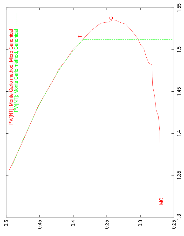
Figure 1: $f(\eta^{R})=PV/[NT]$ as a function of $\eta^{R}$ by Monte Carlo simulations for the microcanonical and canonical ensembles ($N=2000$). Both curves coincide within the statistical error till the point T.

Figure 2: $(\Delta U)^{2}\equiv{{<U^{2}>-<U>^{2}}\over N\;T^{2}}=3\left[f(\eta)-\eta\;f^{\prime}(\eta)-1\right]$ as a function of $\eta$ in the gaseous phase from Monte Carlo simulations with $2000$ particles in the canonical ensemble. Recall that $c_{V}=3/2+(\Delta U)^{2}$.

In the CE, two different phases show up: for $\eta<\eta_{T}$ we have a non-perfect gas and for $\eta>\eta_{T}$ it is a condensed system with negative pressure. The transition between the two phases is very sharp. This phase transition is associated with the Jeans instability.

A negative pressure indicates that the free energy grows for increasing volume at constant temperature [see eq.(57)]. Therefore, the system wants to contract sucking on the walls.

We plot in figs. 1 and 2, $f(\eta)=pV/[NT]$ and $(\Delta U)^{2}$ as functions of $\eta$, respectively.

We find that for small $\eta$, the Monte Carlo results for $pV/[NT]$ well reproduce the analytical formula (107). $pV/[NT]$ monotonically decreases with $\eta$.

In the Monte Carlo simulations the phase transition to the condensed phase happens for $\eta=\eta_{T}$ slightly below $\eta_{C}$. For $N=2000$ we find $\eta_{T}\sim 1.515$. For $\eta_{T}<\eta<\eta_{C}$, the gaseous phase can only exist as a metastable state.

The average distance between particles $<r>$ and the average squared distance between particles $<r^{2}>$ monotonically decrease with $\eta$. When the gas collapses at $\eta_{T}\;,<r>$ and $<r^{2}>$ exhibit a sharp decrease.

The values of $pV/[NT],\;<r>$ and $<r^{2}>$ in the condensed phase are independent of the cutoff for $a<10^{-5}$. The Monte Carlo results in this condensed phase can be approximated for $\eta>2$ as

$${pV\over NT}=f(\eta)\simeq 1-K\;\eta\quad,\quad<r>\simeq 0.016\;.$$ (111)

where $K\simeq 14$.

Since $f(\eta)$ has a jump at the transition, the Gibbs free energy $\Phi$ is discontinuous and we have a phase transition of the zeroth order. We find from eq.(75)

$${\Phi(\mbox{collapse})-\Phi(\eta_{T})\over N\,T}=f(\mbox{collapse})-f(\eta_{T})\simeq-21<0\;.$$ (112)

We can easily compute the latent heat of the transition per particle ($q$) using the fact that the volume $V$ stays constant. Hence, $q=\Delta E/N$ and we obtain from eq.(68)

$${q\over T}={E(\mbox{collapse})-E(\eta_{T})\over N\,T}=3\;\left[f(\mbox{collapse})-f(\eta_{T})\right]\simeq 2-3\,K\;\eta_{T}\simeq-62<0\;.$$ (113)

This phase transition is different from the usual phase transitions since the two phases cannot coexist in equilibrium as their pressures are different.

Eq.(111) can be understood from the general treatment in sec. III as follows. We have from eqs.(60)-(61)

$$f(\eta)=1-{\eta\over 3}<{1\over r}>\;.$$ (114)

The Monte Carlo results indicate that $<{1\over r}>\simeq 42$ is approximately constant in the collapsed region as well as $<r>$ and $<r^{2}>$. Eq.(111) thus follows from eq.(114) using such value of $<{1\over r}>$.

The behaviour of $pV/[NT]$ near $\eta_{C}$ in the gaseous phase can be well reproduced by

$${pV\over NT}=f(\eta)\;\;{\buildrel\eta\uparrow\eta_{C}\over{=}}\;f_{C}+A\;\sqrt{\eta_{C}-\eta}$$ (115)

where $f_{C}\simeq 0.316,\;A\simeq 0.414$ and $\eta_{C}\simeq 1.540$.

In addition, the behaviour of $(\Delta U)^{2}$ in the same region is well reproduced by

$$(\Delta U)^{2}\;\;{\buildrel\eta\uparrow\eta_{C}\over{=}}\;\;C+{D\over\sqrt{\eta_{C}-\eta}}$$ (116)

with $C\simeq-1.64$ and $D\simeq 0.901$. [Notice that for finite $N,\;(\Delta U)^{2}$ will be finite albeit very large at the phase transition]. Eq.(79) relating $f(\eta)$ and $(\Delta U)^{2}$ is satisfied with reasonable approximation.

We thus find a critical region just below $\eta_{C}$ where the energy fluctuations tend to infinity as $\eta\uparrow\eta_{C}$.

The point $\eta_{T}$ where the phase transition actually takes place in the Monte Carlo simulations is at $\eta_{T}\simeq 1.51<\eta_{C}$. This value for $\eta_{T}$ is close to the point $\eta_{0}$ where the isothermal compressibility $\kappa_{T}$ diverges (see sec. VII). They are probably the same point.

Since Monte Carlo simulations are like real experiments, we conclude that the gaseous phase extends from $\eta=0$ till $\eta=\eta_{T}$ in the CE and not till $\eta=\eta_{C}$. Notice that in the literature based on the hydrostatic description of the self-gravitating gas [9, 14, 15, 16], only the instability at $\eta=\eta_{C}$ is discussed whereas the singularities at $\eta=\eta_{0}$ are not considered.

We then performed Monte Carlo calculations in the microcanonical ensemble where the coordinate partition function is given by eq.(18). We thus used

$$\left[\xi+{1\over N}\,u({\vec{r}}_{1},\ldots,{\vec{r}}_{N})\right]^{3N/2-1}\theta\left[\xi+{1\over N}\,u({\vec{r}}_{1},\ldots,{\vec{r}}_{N})\right]\;,$$

as the statistical weight for the Metropolis algorithm.

The MCE and CE Monte Carlo results coincide up to the statistical error for $0<\eta<\eta_{T}$, that is for $\infty>\xi>\xi_{T}\simeq-0.19$. In the MCE the gas does not clump at $\eta=\eta_{C}$ (point $C$ in fig. 1) and the specific heat becomes negative between the points $C$ and $MC$. In the MCE the gas does clump at $\xi\simeq-0.52\;,\;\eta^{T}_{MC}\simeq 1.33$ (point $MC$ in fig. 1) increasing both its temperature and pressure discontinuously. We find from the Monte Carlo data that the temperature increases by a factor $2.4$ whereas the pressure increases by a factor $3.6$ when the gas clumps. The transition point $\eta^{T}_{MC}$ in the Monte Carlo simulations is slightly to the right of the critical point $\eta_{MC}$ predicted by mean field theory. The mean field yields for the sphere $\eta_{MC}=1.2598\ldots$.

In ref.[25] finite $N$ corrections to the critical point $\eta_{MC}$ are computed in mean field for the sphere. This finite $N$ corrections shift $\eta_{MC}$ by $+3.3\%$ for $N=2000$. Since, $\eta^{T}_{MC}$ differs from $\eta_{MC}$ by $+5.6\%$, $\eta^{T}_{MC}$ and $\eta_{MC}$ are probably different critical points.

As is clear, the domain between $C$ and $MC$ cannot be reached in the CE since $c_{V}>0$ in the CE as shown by eq.(78).

We find an excellent agreement between the Monte Carlo and Mean Field (MF) results (both in the MCE and CE). (This happens although the geometry for the MC calculation is cubic while it is spherical for the MF). The points where the collapse phase transition occurs ($\eta_{T}$ and $\eta^{T}_{MC}$) slowly increase with the number of particles $N$.

We verified that the Monte Carlo results in the gaseous phase ($\eta<\eta_{T}$) are cutoff independent for $10^{-3}\geq a\geq 10^{-7}$.

As for the CE, the Gibbs free energy is discontinuous at the transition in the MCE. The transition is then of the zeroth order. We find from eq.(75)

$${\Phi(\mbox{collapse})-\Phi(\eta_{T})\over N\,T_{gas}}={T_{coll}\over T_{gas}}\,f(\mbox{collapse})-f(\eta_{T})\simeq 0.7>0\;.$$

where we used the numerical values from the Monte Carlo simulations. Notice that the Gibbs free energy increases at the MC transition whereas it decreases at the C transition [see eq.(112)].

Here again the two phases cannot coexist in equilibrium since their pressures and temperatures are different.

We display in figs. 3-4 the average particle distribution from Monte Carlo simulations with $2000$ particles in the microcanonical ensemble at both sides of the gravothermal catastrophe, i. e. $\eta=\eta_{MC}$. Fig. 3 corresponds to the gaseous phase and fig. 4 to the collapsed phase. The inhomogeneous particle distribution is clear in fig. 3 whereas fig. 4 shows a dense collapsed core surrounded by a halo of particles.

The different nature of the collapse in the CE and in the MCE can be explained using the virial theorem [see eq.(59)]

$${p\,V\over N\,T}=1+{U\over N\,T}\;.$$

When the gas collapses in the CE the particles get very close and $U$ becomes large and negative while $T$ is fixed. Therefore, $p\,V\over N\,T$ may become large and negative as it does.

We can write the virial theorem also as,

$$p\,V-\frac{1}{2}\,NT=\frac{1}{3}\,E\;.$$

When the gas is near the point MC, $E<0$ is fixed and we have $T>0$. Therefore, $p\,V\over N\,T$ as well as $U=E-3\,N\,T/2$ cannot become large and negative as in the CE collapse. This prevents the distance between the particles to decrease. Actually, the Monte Carlo simulations show that $<r>$ increases by $18\%$ when the gas collapses in the MCE.

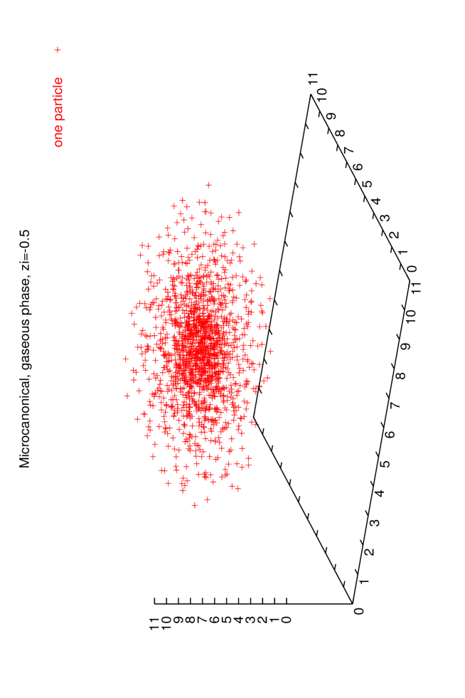
Figure 3: Average particle distribution in the gaseous phase from Monte Carlo simulations with $2000$ particles in the microcanonical ensemble for $\xi=-0.5,\;\eta=1.38,\;pV/[NT]=0.277$.

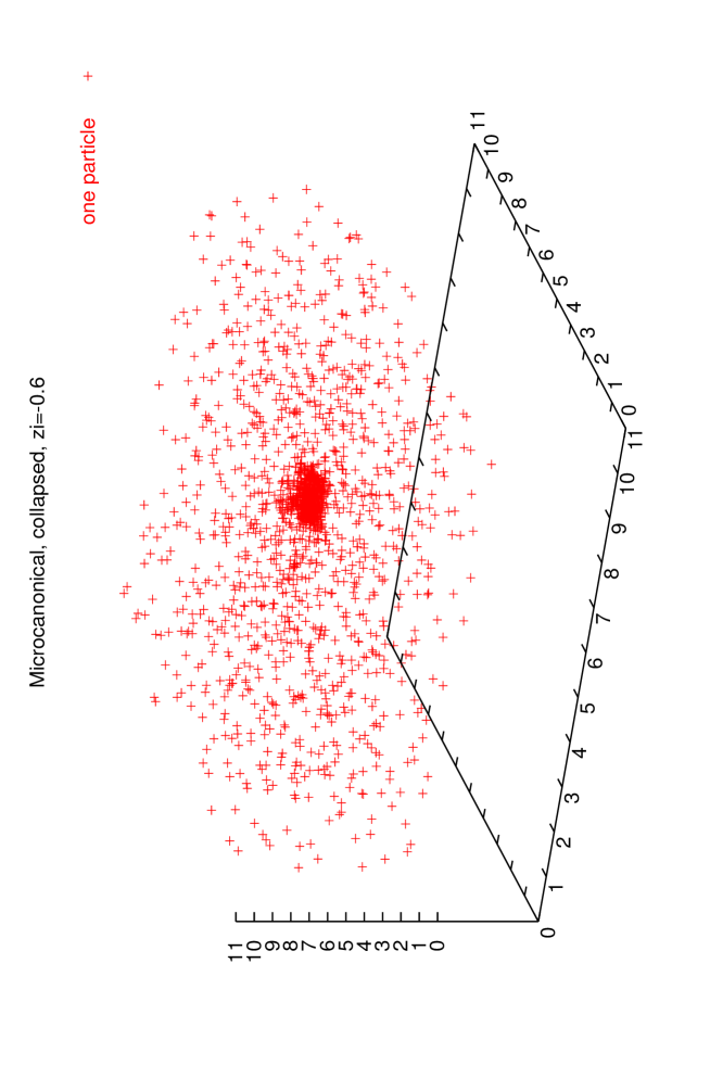
Figure 4: Average particle distribution in the collapsed phase from Monte Carlo simulations with $2000$ particles in the microcanonical ensemble for $\xi=-0.6,\;\eta=0.43,\;pV/[NT]=0.414$.

Figs. 5 and 6 depict the average particle distribution from Monte Carlo simulations with $2000$ particles in the canonical ensemble at both sides of the collapse critical point, i. e. $\eta=\eta_{C}$. Fig. 5 corresponds to the gaseous phase and fig. 6 to the collapsed phase. The inhomogeneous particle distribution is clear in fig. 5 whereas fig. 6 shows a dense collapsed core surrounded by a very little halo of particles.

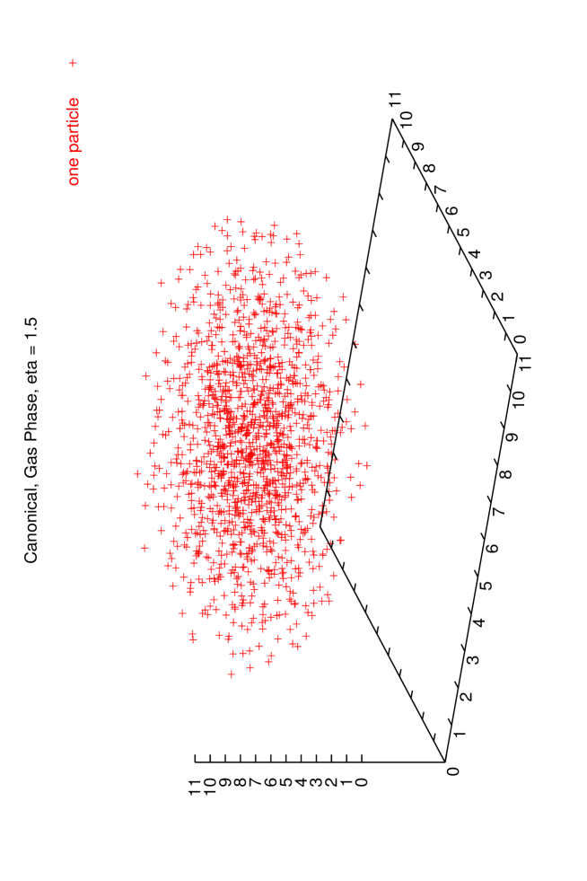
Figure 5: Average particle distribution in the gaseous phase from Monte Carlo simulations in the canonical ensemble for $\eta=1.5$ and $N=2000$

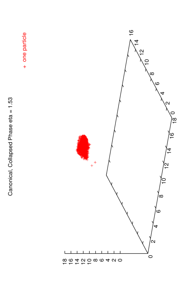
Figure 6: Average particle distribution in the collapsed phase from Monte Carlo simulations with $2000$ particles in the canonical ensemble for $\eta=1.53,\;pV/[NT]=-14.44$.

Notice that the collapsed phases are of different nature in the CE and MCE. The core is much tighter and the halo much smaller in the CE than in the MCE.

Figs. 3 and 5 depict the average particle distribution for the gaseous phase in the MCE and the CE, respectively. In this phase, the MC simulations give identical descriptions for large $N$ in both ensembles. [This important point will be further demostrated in sec. VI by functional integral methods]. The average configurations in figs. 3 and 5 describe a self-gravitating gas in thermal equilibrium within a cube. We may call it the isothermal cube by analogy with the well known isothermal sphere[10]-[16].

6 Mean Field Approach

Both in the microcanonical and the canonical ensembles the coordinate partition functions are given by $3N$-uple integrals [eqs.(18) and (56), respectively]. In the $N\to\infty$ limit both $3N$-uple integrals can be recasted as functional integrals over the continuous particle density as we see below.

6.1 The Canonical Ensemble

We now recast the coordinate partition function $e^{\Phi_{N}(\eta)}$ in the canonical ensemble given by eq.(56) as a functional integral in the thermodynamic limit.

$$e^{\Phi_{N}(\eta)} \buildrel N>>1\over{=} \int\int D\rho\;d{\hat{a}}\;e^{-Ns_{C}[\rho(.),\hat{a},\eta]}$$ (117)

$$s_{C}[\rho(.),\hat{a},\eta] = -{\eta\over 2}\int{d^{3}x\;d^{3}y\over|{\vec{x}}-{\vec{y}}|}\;\rho({\vec{x}})\;\rho({\vec{y}})+\int d^{3}x\;\rho({\vec{x}})\;\log\rho({\vec{x}})-i{\hat{a}}\left(\int d^{3}x\,\rho({\vec{x}})-1\right)\;.$$

where we used the coordinates $\vec{x}$ in the unit volume. The first term is the potential energy, the second term is the functional integration measure for this case (see appendix A). Here $N\;\rho({\vec{x}})$ stands for the density of particles.

The integration over $\hat{a}$ enforces the number of particles to be exactly $N$:

$$\int d^{3}x\;\rho({\vec{x}})=1$$ (119)

That is, in the coordinates $\vec{q}$ (running from $0$ to $L$), the density of particles is

$${N\over L^{3}}\;\rho({\vec{q}})\quad{\rm with}\quad\int d^{3}q\;{N\over L^{3}}\;\rho({\vec{q}})=N\;.$$

6.2 The Microcanonical Ensemble

Let us express the coordinate partition function in the microcanonical ensemble $w(\xi,N)$ defined by eq.(18) in terms of the coordinate partition function in the canonical ensemble $e^{\Phi_{N}(\eta)}$ defined by eq.(56). In order to do that we use the Fourier expansion [23]

$$x^{\lambda}\;\theta(x)={\Gamma(\lambda+1)\over 2\pi}\int_{-\infty}^{+\infty}e^{i\,\omega\,x}{d\omega\over(i\omega)^{\lambda+1}}$$ (120)

We thus find from eqs.(18), (56) and (120) that

$$w(\xi,N) = \Gamma\left({3N\over 2}\right)\int_{-\infty}^{+\infty}{d\omega\over 2\pi}\;e^{i\omega\xi+\Phi_{N}(i\omega/N)-{3N\over 2}\log(i\omega)}$$ (121)

$$= N\,\Gamma\left({3N\over 2}\right)\int_{\gamma}{d\eta\over 2\pi i}\;e^{N\,\eta\,\xi+\Phi_{N}(\eta)-{3N\over 2}\log(N\,\eta)}$$ (123)

where we introduced the integration variable $\eta\equiv i\omega/N$ and where $\gamma$ is an upward integration contour parallel to the imaginary $\eta$ axis. Using Stirling’s approximation for the $\Gamma$ function we find for $N\gg 1$ up to irrelevant constants

$$w(\xi,N)\buildrel N>>1\over{=}\int_{\gamma}{d\eta\over 2\pi i}\;e^{N\,\eta\,\xi+\Phi_{N}(\eta)-{3N\over 2}\log\eta}$$

Now, inserting the functional integral representation (117) for the coordinate canonical partition function yields,

$$w(\xi,N)\buildrel N>>1\over{=}\int\int D\rho\;d{\hat{a}}\;{d\eta\over 2\pi i}\;e^{N\left[\eta\,\xi-{3\over 2}\log\eta-s_{C}[\rho(.),\hat{a},\eta]\right]}$$ (124)

We thus find a functional integral representation in the microcanonical ensemble analogous to the canonical representation eq.(117) but with an extra integration (over $\eta$) that constrains the value of the energy.

The ‘effective action’ in the microcanonical ensemble takes thus the form,

$$s_{MC}[\rho(.),\hat{a},\eta]={3\over 2}\log\eta-\eta\,\xi-{\eta\over 2}\int{d^{3}x\;d^{3}y\over|{\vec{x}}-{\vec{y}}|}\;\rho({\vec{x}})\;\rho({\vec{y}})+\int d^{3}x\;\rho({\vec{x}})\;\log\rho({\vec{x}})-i{\hat{a}}\left(\int d^{3}x\,\rho({\vec{x}})-1\right)$$ (125)

6.3 The Grand Canonical Ensemble

The partition function in the grand canonical ensemble can be written as

$${\cal Z}_{GC}(z,T)=\sum_{N=0}^{\infty}z^{N}\;{\cal Z}(N,T)\;,$$ (126)

where $z=e^{\mu\over T}$ stands for the fugacity and ${\cal Z}(N,T)$ is the partition function in the canonical ensemble given by eqs.(49) and (52).

As shown in ref.[4], this grand canonical partition function can be expressed as a functional integral

$${\cal Z}_{GC}(z,T)=\int\int\;{\cal D}\Phi\;e^{{1\over{T_{eff}}}\;\int_{V}d^{3}q\left[\frac{1}{2}\Phi\;\nabla^{2}\Phi\;+M^{2}\;e^{\Phi({\vec{q}})}\right]}\;,$$ (127)

where

$$M^{2}=\sqrt{2\;T\over{\pi}}\;z\;G\,m^{7/2}\quad,\quad T_{eff}=4\pi\;{{G\;m^{2}}\over{T}}\;.$$ (128)

Notice that the representation (127) is exact while the functional integral representations in the microcanonical and canonical ensembles only apply for large number of particles.

Rewriting eq.(127) in terms of the dimensionless variables (11) yields for the exponent

$${1\over{T_{eff}}}\;\int_{V}d^{3}q\left[\frac{1}{2}\Phi\;\nabla^{2}_{q}\Phi\;+\mu^{2}\;e^{\Phi({\vec{q}})}\right]={L\over T_{eff}}\;\int_{0}^{1}d^{3}x\left[\frac{1}{2}\Phi\;\nabla^{2}_{r}\Phi\;+\zeta^{2}\;e^{\Phi({\vec{x}})}\right]$$

where $\zeta\equiv M\;L$ is of the order one ($L^{0}$), since $M^{2}\sim z=e^{\mu\over T}\sim L^{-2}$ [see eq.(70)].

Since the exponent in the functional integral (127) is proportional to $L$, the large volume limit is dominated by the stationary points (mean field approximation)

$$\nabla^{2}_{r}\Phi_{s}({\vec{x}})\;+\zeta^{2}\;e^{\Phi_{s}({\vec{x}})}=0\;.$$ (129)

We expand around the saddle point $\Phi_{s}({\vec{x}})$ changing to a new functional integration $Y({\vec{x}})$ variable as follows,

$$\Phi({\vec{x}})=\Phi_{s}({\vec{x}})+Y({\vec{x}})\;.$$ (130)

Keeping in eq.(127) quadratic terms in $Y(.)$ yields,

$${\cal Z}_{GC}(z,T)=e^{{L\over T_{eff}}\;\int_{0}^{1}d^{3}x\left[\frac{1}{2}\Phi_{s}\;\nabla^{2}_{r}\Phi_{s}\;+\zeta^{2}\;e^{\Phi_{s}({\vec{x}})}\right]}\;\int\int\;{\cal D}Y\;e^{{L\over 2\;T_{eff}}\;\int_{0}^{1}d^{3}x\;\left[Y\nabla^{2}Y+\zeta^{2}\,Y^{2}\;e^{\Phi_{s}({\vec{x}})}\right]}\left[1+{\cal O}\left({1\over L}\right)\right]$$ (131)

where the Gaussian integral over $Y(.)$ gives a factor of order $L^{0}$ [see paper II].

We recall that the saddle point method applies while all eigenvalues of the quadratic form in the exponent of eq.(131) are positive. Therefore, the determinant of the quadratic fluctuations is positive. The determinant vanishing or changing sign indicates the presence of zero or negative eigenvalues. In such a case the system is no more on a stable phase but on a metastable or unstable phase. The free energy gets an imaginary part in such metastable or unstable situations.

The average number of particles in the grand canonical ensemble is given by

$${\bar{N}}={1\over{\cal Z}_{GC}}\sum_{N=0}^{\infty}Nz^{N}\;{\cal Z}(N,T)=\left.{\partial\log{\cal Z}_{GC}\over\partial\log z}\right|_{V,T}\;.$$

We thus find in the mean field approximation,

$${\bar{N}}={L\;\zeta^{2}\over T_{eff}}\int_{0}^{1}d^{3}x\;e^{\Phi_{s}({\vec{x}})}$$

Therefore, using this and eq.(128) we can express $\zeta^{2}$ in terms of $\eta$ where we denote $\bar{N}$ as $N$ to avoid cluttering of notation,

$$\zeta^{2}={4\pi\eta\over\int_{0}^{1}d^{3}x\;e^{\Phi_{s}({\vec{x}})}}\;,$$ (132)

and the fugacity results

$$z={N\over L^{3}}\left({2\pi\over mT}\right)^{3/2}{1\over\int_{0}^{1}d^{3}x\;e^{\Phi_{s}({\vec{x}})}}\;.$$ (133)

We again see that $z\sim L^{-2}$ in the GCE.

Integrating eq.(129) over the unit volume yields

$$\int{\vec{\nabla}}\Phi_{s}({\vec{x}})\cdot d{\vec{s}}=-4\pi\eta$$ (134)

where we used eq.(132).

We find for the free energy[2],

$$F=-T\log{\cal Z}_{GC}+NT\;\log z=F_{0}+{NT\over 2}K(\eta)-NT\,\log C(\eta)+{\cal O}(N^{0})\;,$$ (135)

where we used the grand canonical partition function (131) evaluated at the stationary point,

$$\log{\cal Z}_{GC}=N\left[1-\frac{1}{2}\,K(\eta)\right]\;,$$ (136)

and $z$ is given by eq.(133) with

$$K(\eta)\equiv{\int_{0}^{1}d^{3}x\;\Phi_{s}({\vec{x}})\;e^{\Phi_{s}({\vec{x}})}\over C(\eta)}\quad\mbox{and}\quad C(\eta)\equiv\int_{0}^{1}d^{3}x\;e^{\Phi_{s}({\vec{x}})}\;.$$ (137)

$F_{0}$ is given by eq.(67).

We easily calculate the mean value of the potential energy in the mean field approximation

$$<U>=-T\;{\partial\log{\cal Z}_{GC}\over\partial\log G}=-{NT\over 2}K(\eta)$$ (138)

Combining the two expressions for the entropy

$$S={E-F\over T}\quad\mbox{and}\quad S=-\left({\partial F\over\partial T}\right)_{V}\;,$$ (139)

yields

$$S=S_{0}-N\left[K(\eta)-\log C(\eta)\right]$$ (140)

and the first order differential equation

$$\eta\,K^{\prime}(\eta)+K(\eta)=2\,\eta{d\over d\eta}\log C(\eta)\;.$$ (141)

The boundary conditions $K(0)=0,\;C(0)=1$ ensure the ideal gas limit $\eta=0$.

The pressure takes the form,

$$P=-\left({\partial F\over\partial V}\right)_{T}={NT\over V}\left[1+{\eta\over 3}\;\left(\frac{1}{2}K^{\prime}(\eta)-{d\over d\eta}\log C(\eta)\right)\right]+{\cal O}(N^{0})\;.$$ (142)

These equations guarantee in addition that the virial theorem (59) holds.

6.4 Saddle point evaluation in the canonical ensemble

The functional integral in eq.(117) is dominated for large $N$ by the extrema of the ‘effective action’ $s_{C}[\rho(.),\hat{a},\eta]$, that is, the solutions of the stationary point equation

$$\log\rho_{s}({\vec{x}})-\eta\int{d^{3}y\;\rho_{s}({\vec{y}})\over|{\vec{x}}-{\vec{y}}|}=a_{s}\;,$$ (143)

$a=i{\hat{a}}$ is a Lagrange multiplier enforcing the constraint (119).

Applying the Laplacian and setting $\phi({\vec{x}})\equiv\log\rho_{s}({\vec{x}})$ yields,

$$\nabla^{2}\phi({\vec{x}})+4\pi\eta\;e^{\phi({\vec{x}})}=0\;,$$ (144)

This equation is scale covariant [4]. That is, if $\phi({\vec{x}})$ is a solution of eq.(144), then

$$\phi_{\lambda}({\vec{x}})\equiv\phi(\lambda{\vec{x}})+\log\lambda^{2}$$ (145)

where $\lambda$ is an arbitrary constant is also a solution of eq.(144). For spherically symmetric solutions this property can be found in ref.[8].

Integrating eq.(144) over the unit volume and using the constraint (119) yields

$$\int{\vec{\nabla}}\phi({\vec{x}})\cdot d{\vec{s}}=-4\pi\eta$$ (146)

where the surface integral is over the boundary of the unit volume.

Comparing eqs.(129)-(134) with (144) and (146) shows that the grand canonical and canonical stationary points are related by

$$\Phi_{s}({\vec{x}})=\phi({\vec{x}})+\log C(\eta)\;.$$ (147)

Eq.(131) can then be written as

$${\cal Z}_{GC}(z,T)=e^{{N\over 4\pi\eta}\;\left\{\int_{0}^{1}d^{3}x\left[\frac{1}{2}\phi\;\nabla^{2}_{r}\phi\;+4\pi\eta\;e^{\phi({\vec{x}})}\right]-2\pi\eta\log C(\eta)\right\}}\times$$ (148)

(149)

$$\int\int\;{\cal D}Y\;e^{{N\over 8\pi\eta}\;\int_{0}^{1}d^{3}x\;\left[Y\nabla^{2}Y+4\pi\eta\,Y^{2}\;e^{\phi({\vec{x}})}\right]}\left[1+{\cal O}\left({1\over N}\right)\right]$$ (150)

where we used eqs.(53), (128), (132) , (146) and (147).

We have taken the zero cutoff limit in eqs.(143)-(144). The mean field equations turn to be finite with regular solutions in such limit. This can be understood from our perturbative calculation in sec. III.A. All potentially divergent contributions at zero cutoff are suppressed by factors $1/N^{2}$ and therefore disappear in the $N=\infty$ limit. Hence one can set the cutoff to zero in the mean field approximation.

In order to evaluate the functional integral in eq.(117) by the saddle point method we change the functional integration variable as follows,

$$\rho({\vec{x}})=\rho_{s}({\vec{x}})+Y({\vec{x}})\quad,\quad a=a_{s}+y_{0}$$ (151)

where $\rho_{s}({\vec{x}})$ and $a_{s}$ obey eq.(143). We can expand the exponent to second order as

$$s_{C}[\rho(.),a,\eta]-s_{C}[\rho_{s}(.),a_{s},\eta]=s^{(2)}_{C}[Y(.),y_{0}]+{\cal O}\left(Y^{3},Y^{2}\,y_{0}\right)$$ (152)

where we use that

$$\left.{\delta s_{C}\over\delta\rho({\vec{x}})}\right|_{\rho=\rho_{s},\,a=a_{s}}=0\quad,\quad\left.{\partial s_{C}\over\partial a}\right|_{\rho=\rho_{s},\,a=a_{s}}=0$$

and

$$\left.\left.s^{(2)}_{C}[Y(.),y_{0}]\equiv\frac{1}{2}\int d^{3}x\;d^{3}y\;Y({\vec{x}})\;Y({\vec{y}})\;{\delta^{2}s_{C}\over\delta\rho({\vec{x}})\delta\rho({\vec{y}})}\right|_{\rho=\rho_{s},\,a=a_{s}}+y_{0}\;\int d^{3}x\;Y({\vec{x}})\;{\delta^{2}s_{C}\over\delta\rho({\vec{x}})\partial a}\right|_{\rho=\rho_{s},\,a=a_{s}}\;.$$

Notice that

$${\partial^{2}s_{C}\over\partial a^{2}}=0\;.$$

We evaluate explicitly the second derivatives from eq.(117) with the result,

$${\delta^{2}s_{C}\over\delta\rho({\vec{x}})\;\delta\rho({\vec{y}})}={\delta(\vec{x}-\vec{y})\over\rho({\vec{x}})}-{\eta\over|\vec{x}-\vec{y}|}\quad,\quad{\delta^{2}s_{C}\over\delta\rho({\vec{x}})\;\partial a}=1$$

Therefore,

$$s^{(2)}_{C}[Y(.),y_{0}]=\frac{1}{2}\;\int d^{3}x\;{Y^{2}({\vec{x}})\over\rho({\vec{x}})}-{\eta\over 2}\int{d^{3}x\;d^{3}y\over|{\vec{x}}-{\vec{y}}|}\;Y({\vec{x}})\;Y({\vec{y}})-y_{0}\;\int d^{3}x\;Y({\vec{x}})$$ (153)

Inserting eqs.(151) and (152) into eq.(117) yields

$$e^{\Phi_{N}(\eta)}\buildrel N>>1\over{=}e^{-N\,s(\eta)}\;\int\int DY\,dy_{0}\;e^{-N\,s^{(2)}_{C}[Y(.),y_{0}]}\;\left[1+{\cal O}\left({1\over N}\right)\right]$$ (154)

where $s(\eta)\equiv s_{C}[\rho_{s}(.),a_{s},\eta]$ stands for the value of the exponent at the saddle point. Terms of order higher than quadratic in $s_{C}[\rho(.),a,\eta]$ contribute to the $1/N$ corrections.

The Gaussian functional integral (154) can be exactly computed in terms of the functional determinant of the quadratic form (153) [see paper II]. It gives a result of order one ($N^{0}$).

In the mean field approximation we only keep the dominant order for large $N$. Therefore, only the exponent at the saddle point accounts and according to eq.(55) we find for the free energy

$$F = F_{0}+N\,T\,s(\eta)+{\cal O}(N^{0})$$ (155)

$${pV\over NT} = 1+{\eta\over 3}{ds\over d\eta}+{\cal O}(N^{-1})$$ (157)

Hence, in the mean field approximation, the function $f(\eta)$ is given by

$$f_{MF}(\eta)\equiv 1+{\eta\over 3}{ds\over d\eta}\;,$$ (158)

From eq.(117) we can compute $s(\eta)$ in terms of the saddle point solution as follows

$$s(\eta)\equiv s_{C}[\rho_{s}(.),a_{s},\eta]=-{\eta\over 2}\int{d^{3}x\;d^{3}y\over|{\vec{x}}-{\vec{y}}|}\;\rho_{s}({\vec{x}})\;\rho_{s}({\vec{y}})+\int d^{3}x\;\rho_{s}({\vec{x}})\;\log\rho_{s}({\vec{x}})\;.$$ (159)

Using eq.(143) we find an equivalent expression that will be useful in paper II,

$$s(\eta)={a_{s}\over 2}+\frac{1}{2}\int\phi({\vec{x}})\;e^{\phi({\vec{x}})}\;d^{3}x\;.$$ (160)

6.5 Saddle point evaluation in the microcanonical ensemble

The extrema of the ‘effective action’ (125) dominate the microcanonical partition function (124) in the large $N$ limit. Extremizing eq.(125) with respect to $\rho(.)$ and $\hat{a}$ gives again eqs.(143) and (119), respectively.

An extra equation follows by extremizing the ‘effective action’ (125) with respect to $\eta$:

$$\xi={3\over 2\,\eta_{s}}-{1\over 2}\int{d^{3}x\;d^{3}y\over|{\vec{x}}-{\vec{y}}|}\;\rho_{s}({\vec{x}})\;\rho_{s}({\vec{y}})$$ (161)

Going back to dimensionful variables this equation takes the familiar form

$$E=\frac{3}{2}NT-{G\,m^{2}\over 2}\int{d^{3}q\;d^{3}q^{\prime}\over|{\vec{q}}-{\vec{q}}\,^{\prime}|}\;N\rho({\vec{q}})\;N\rho({\vec{q}}\,^{\prime})$$

That is, eq.(161) enforces the fixed value of the energy in the microcanonical ensemble.

Therefore, the stationary point equations in the microcanonical and canonical ensembles are identical. Both ensembles yield the same results in the $N\to\infty$ limit in their common region of validity. We derive the domain of validity of the mean field approach for each of the three statistical ensembles in paper II. That is, the regions where all fluctuations around it decrease its statistical weight within their common region of validity.

In order to evaluate the functional integral for the microcanonical partition function (124)

$$w(\xi,N)\buildrel N>>1\over{=}\int\int D\rho\;d{\hat{a}}\;{d\eta\over 2\pi i}\;e^{-Ns_{MC}[\rho(.),\hat{a},\eta]}$$ (162)

we expand the ‘effective action’ $s_{MC}[\rho(.),\hat{a},\eta]$ around the stationary point $\rho_{s}(.),{\hat{a}}_{s},\eta_{s}$ to second order. This gives

$$w(\xi,N)\buildrel N>>1\over{=}e^{-N\,s(\eta)}\;\int\int DY\,dy_{0}\;{d{\tilde{\eta}}\over 2\pi i}\;e^{-N\,s^{(2)}_{MC}[Y(.),y_{0},{\tilde{\eta}}]}\;\left[1+{\cal O}\left({1\over N}\right)\right]$$ (163)

where $Y(.)$ and $y_{0}$ are defined by eq.(151) and we set $\eta=\eta_{s}+{\tilde{\eta}}$. The second order piece of the ‘effective action’ takes now the form

$$s^{(2)}_{MC}[Y(.),y_{0},{\tilde{\eta}}]=s^{(2)}_{C}[Y(.),y_{0}]-{\tilde{\eta}}\int{d^{3}x\;d^{3}y\over|{\vec{x}}-{\vec{y}}|}\;\rho_{s}({\vec{x}})\;Y({\vec{y}})-{3\over 4\,\eta_{s}^{2}}\,{\tilde{\eta}}^{2}\;.$$ (164)

The Gaussian functional integral in eq.(163) yields a contribution of order one ($N^{0}$) [see paper II]. The dominant (mean field) contribution, $e^{-N\,s(\eta)}$, exactly coincides with the mean field result in the canonical ensemble [eq.(154)] Therefore, the canonical and microcanonical ensembles yields identical physical magnitudes and the same equation of state in the mean field limit.

6.6 Spherically symmetric case

We shall consider here the spherically symmetric case where eq.(144) takes the form

$${d^{2}\phi\over dR^{2}}+\frac{2}{R}{d\phi\over dR}+4\pi\eta\;e^{\phi(R)}=0\;.$$ (165)

where we work on an unit volume sphere instead of an unit volume cube as in eq.(11). Therefore, the radial variable runs in the interval

$$0\leq R\leq\left({3\over 4\pi}\right)^{1/3}$$

It is more convenient to introduce a new radial variable

$$r\equiv R\left({4\pi\over 3}\right)^{1/3}$$

such that $0\leq r\leq 1$.

The saddle point equation (165) takes then the form

$${d^{2}\phi\over dr^{2}}+\frac{2}{r}{d\phi\over dr}+4\pi\eta^{R}\;e^{\phi(r)}=0\;.$$ (166)

where

$$\eta^{R}\equiv\eta\;\left({4\pi\over 3}\right)^{1/3}=1.61199\ldots\;\eta\quad\mbox{and}\quad e^{\phi(r)}=e^{\phi(R)}\;{3\over 4\pi}\;.$$ (167)

In order to have a regular solution at $r=0$ one has to impose

$$\phi^{\prime}(0)=0\;.$$ (168)

Otherwise, the second term in eq.(165) diverges for $r\to 0$.

In the spherically symmetric case, the constraint (146) becomes

$$\phi^{\prime}(1)=-\eta^{R}\;.$$ (169)

Figure 7: $\eta^{R}$ as a function of the uniformizing scale variable $\log\lambda$ according to eq.(173). Notice the maximum of $\eta^{R}$ as $\eta_{C}^{R}=2.517551\ldots$. The region beyond the point MC, ($\ln\lambda_{MC}=3.53698\ldots$), is unphysical as we discuss in paper II

Using the scale covariance (145) we can express $\phi(r)$ as

$$\phi(r)=\log\left({\lambda^{2}\over 4\,\pi\,\eta^{R}}\right)+\chi(\lambda\,r)$$ (170)

where

$$\chi^{\prime\prime}(\lambda)+{2\over\lambda}\,\chi^{\prime}(\lambda)+e^{\chi(\lambda)}=0\quad,\quad\chi^{\prime}(0)=0$$ (171)

This equation is invariant under the transformation:

$$\lambda\Rightarrow\lambda\;e^{\alpha}\quad\,\quad\chi(\lambda)\Rightarrow\chi(\lambda)-2\;\alpha\;,$$ (172)

where $\alpha$ is a real number. Hence, we can set $\chi(0)\equiv 0$ without loosing generality.

$\chi(x)$ is independent of $\eta^{R}$, and $\lambda$ is related to $\eta^{R}$ through eq.(169)

$$\lambda\;\chi^{\prime}(\lambda)=-\eta^{R}\;.$$ (173)

Since $\lambda$ and $\eta^{R}$ are always positive, $\chi(\lambda)$ is a monotonically decreasing function of $\lambda$.

Eq.(171) can be easily solved for small arguments as

$$\chi(x)=-{x^{2}\over 6}+{x^{4}\over 120}+{\cal O}(x^{6})$$

Hence, in the dilute limit eq.(173) relating $\eta^{R}$ with $\lambda$ gives

$$\eta^{R}={\lambda^{2}\over 3}-{\lambda^{4}\over 30}+{\cal O}(\lambda^{6})\;.$$ (174)

For large argument, the solution of eq.(171) takes the asymptotic form[8]

$$\chi(x)=\log{2\over x^{2}}+{A\over\sqrt{x}}\cos\left({\sqrt{7}\over 2}\log{x}+B\right)\left[1+{\cal O}\left({1\over x}\right)\right]$$ (175)

where $A$ and $B$ are numerical constants. Using eq.(173) this gives for $\eta^{R}$

$$\eta^{R}=2+{C\over\sqrt{\lambda}}\cos\left({\sqrt{7}\over 2}\log{\lambda}+D\right)\left[1+{\cal O}\left({1\over\lambda}\right)\right]$$ (176)

where $C$ and $D$ are constants related to $A$ and $B$. By numerically solving eq.(171) we find

$$C=1.667\ldots\;.$$

It must be noticed, however, that the mean field solution is unphysical for $\lambda>\lambda_{MC}=34.36361\ldots$ as we shall see in paper II. Anyway, we see from fig. 7 that $\eta^{R}$ approaches very fast its asymptotic behaviour (176) for $\log\lambda>2$.

We plot in fig. 8 $\chi(\lambda(\eta^{R}))$ as a function of $\eta^{R}$.

In the spherically symmetric case the integral over the angles in eq.(143) is immediate with the result,

$$\phi(r)=a_{s}+4\pi\eta^{R}\left[{1\over r}\int_{0}^{r}{r}^{\prime\,2}\;dr^{\prime}\;e^{\phi(r^{\prime})}+\int_{r}^{1}r^{\prime}\;dr^{\prime}\;e^{\phi(r^{\prime})}\right]$$ (177)

Deriving with respect to $r$ yields,

$${d\phi(r)\over dr}=-\frac{4\pi\eta^{R}}{r^{2}}\int_{0}^{r}{r^{\prime}}^{\,2}\;dr^{\prime}\;e^{\phi(r^{\prime})}$$

This again shows that $\phi(r)$ is a monotonically decreasing function of $r$ [see above, eq.(173)].

Setting $r=1$ in eq.(177) leads to the relation

$$\phi(1)=a_{s}+4\pi\eta^{R}\int_{0}^{1}r^{2}\;dr\;e^{\phi(r)}$$

Using now the constraint (119) allows us to compute the Lagrange multiplier $a$ at the saddle point

$$a_{s}=\phi(1)-\eta^{R}$$ (178)

The particle density in MF is given by

$$\rho(r)=e^{\phi(r)}={\lambda^{2}\over 4\,\pi\,\eta^{R}}\;e^{\chi(\lambda\,r)}\;,\;0\leq r\leq 1\;.$$

Since $\chi(\lambda)$ monotonically decreases with $\lambda$, the particle density monotonically decreases with $r$ for fixed $\eta^{R}$.

Figure 8: $\chi(\lambda(\eta^{R}))=\log{p(0)\over p(1)}=\log{\rho(0)\over\rho(1)}$ as a function of $\eta^{R}$.

Let us now compute $s(\eta^{R})$ [the exponent in eq.(117) at the saddle point] for the spherically symmetric case. We find from eq.(160)

$$s(\eta^{R}) = \frac{1}{2}\left[\phi(1)-\eta^{R}\right]+2\pi\int_{0}^{1}r^{2}\;dr\;\phi(r)\;e^{\phi(r)}$$ (179)

$$= \log\left({\lambda^{2}\over 4\,\pi\,\eta^{R}}\right)+\chi(\lambda)-{\eta^{R}\over 2}+{1\over 2\;\lambda\;\eta^{R}}\int_{0}^{\lambda}x^{2}\;dx\;[\chi^{\prime}(x)]^{2}$$ (181)

where we integrated by parts and used eqs.(170)-(173).

The integral in the r.h.s. of eq.(179) can be computed in closed form [see appendix B] with the result,

$$s(\eta^{R})=\log\left({\lambda^{2}\over 4\,\pi\,\eta^{R}}\right)+\chi(\lambda)+3-\eta^{R}-{\lambda^{2}\over\eta^{R}}\;e^{\chi(\lambda)}$$

Inserting now $s(\eta^{R})$ into eq.(158) and using eqs.(171)-(173) yields after calculation

$$f_{MF}(\eta^{R}) = {\lambda^{2}\over 3\,\eta^{R}}\;e^{\chi(\lambda)}\quad,$$ (182)

$$s(\eta^{R}) = 3[1-f_{MF}(\eta^{R})]-\eta^{R}+\log\left[{3f_{MF}(\eta^{R})\over 4\pi}\right]$$

Notice that $f_{MF}(\eta^{R})$ as well as the other physical quantities are invariant under the transformation (172) as it must be.

Figure 9: $f_{MF}(\eta^{R})=PV/[NT]$ as a function of $\eta^{R}$ in the MF approximation [eq.(184)]. $f_{MF}(\eta^{R})$ has a square root branch point at $\eta^{R}_{C}$. The points GC, C and MC indicate the transition to the collapsed phase for each ensemble (grand canonical, canonical and microcanonical, respectively): $\eta^{R}_{GC}=0.797375\ldots,\;\eta^{R}_{C}=2.517551\ldots,\;\eta^{R}_{MC}=2.03085\ldots$ (notice that $\eta^{R}_{MC}$ is in the second Riemann sheet). Since $E/[3NT]=f_{MF}(\eta^{R})-\frac{1}{2}$, this plot also shows the energy per particle as a function of $\eta^{R}$. Furthermore, the particle density at the surface is proportional to $f_{MF}(\eta^{R})$ [eq.(185)].

It follows from eqs.(171), (173) and (182) that $f_{MF}(\eta^{R})$ obeys the first order non-linear differential equation

$$\eta^{R}(3f_{MF}-1)f^{\prime}_{MF}(\eta^{R})+(3f_{MF}-3+\eta^{R})f_{MF}=0\;.$$ (184)

which reduces to an Abel equation of first kind[22].

We thus find that in the mean field approximation all thermodynamic quantities follow from the resolution of the single first order non-linear differential eq.(184) with the initial condition $f_{MF}(0)=1$.

Integrating eq.(184) with respect to $\eta^{R}$ yields,

$$3\int_{0}^{\eta^{R}}{dx\over x}[1-f_{MF}(x)]=3[f_{MF}(\eta^{R})-1]+\eta^{R}-\log f_{MF}(\eta^{R})$$

Further useful relations follow from eqs.(170) and (182)

$$\phi(1)=\log\left[{3\,f_{MF}(\eta^{R})\over 4\,\pi}\right]\quad,\quad\rho(1)={3\over 4\,\pi}\;f_{MF}(\eta^{R})\;.$$ (185)

That is, the particle density at the surface ($r=1$) is proportional to $f_{MF}(\eta^{R})$.

We can then write the different physical magnitudes in the MF approximation as

$${pV\over NT} = f_{MF}(\eta^{R})$$ (186)

$${F-F_{0}\over NT} = 3[1-f_{MF}(\eta^{R})]-\eta^{R}+\log f_{MF}(\eta^{R})$$ (188)

$${S-S_{0}\over N} = 6[f_{MF}(\eta^{R})-1]+\eta^{R}-\log f_{MF}(\eta^{R})$$ (190)

$${E\over NT} = 3[f_{MF}(\eta^{R})-\frac{1}{2}]$$

where we used eqs.(64), (66), (68) and (72).

We derive in appendix C the properties of the function $f_{MF}(\eta^{R})$ from the differential equation (184). One easily obtains for small $\eta^{R}$ (dilute regime),

$$f_{MF}(\eta^{R})=1-\frac{\eta^{R}}{5}-\frac{(\eta^{R})^{2}}{175}+{\cal O}([\eta^{R}]^{3})\;.$$

These terms exactly coincide with the perturbative calculation in the dilute regime for spherical symmetry [see eq.(40), (107) and (167)].

We plot in fig. 1 $f_{MF}(\eta^{R})$ as a function of $\eta^{R}$ obtained by solving eq.(184) by the Runge-Kutta method. We see that $f_{MF}(\eta^{R})$ is a monotonically decreasing function of $\eta^{R}$ for $0<\eta^{R}<\eta^{R}_{C}$. At the point $\eta^{R}=\eta^{R}_{C}$, the derivative $f_{MF}^{\prime}(\eta^{R})$ takes the value $-\infty$. It then follows from eq.(184) that

$$f_{MF}(\eta^{R}_{C})=\frac{1}{3}\;.$$

At the point $\eta^{R}_{C}$ the series expansion for $f_{MF}(\eta^{R})$ in powers of $\eta^{R}$ diverges. Both, from the ratio test on its coefficients and from the Runge-Kutta solution, we find that

$$\eta^{R}_{C}=2.517551\ldots$$ (192)

From eq.(184) we find that $f_{MF}(\eta^{R})-\frac{1}{3}$ has a square root behaviour around $\eta^{R}=\eta^{R}_{C}$:

$$f_{MF}(\eta^{R})\buildrel\eta^{R}\uparrow\eta^{R}_{C}\over{=}\frac{1}{3}+\sqrt{2(\eta^{R}_{C}-2)\over 9\,\eta^{R}_{C}}\;\sqrt{\eta^{R}_{C}-\eta^{R}}+{2\,(\eta^{R}_{C}-1)\over 7\,\eta^{R}_{C}}\;(\eta^{R}_{C}-\eta^{R})+{\cal O}\left[(\eta^{R}_{C}-\eta^{R})^{3/2}\right]$$

Inserting the numerical value (192) for $\eta^{R}_{C}$ yields,

$$f_{MF}(\eta^{R})\buildrel\eta^{R}\uparrow\eta^{R}_{C}\over{=}\frac{1}{3}+0.213738\ldots\sqrt{\eta^{R}_{C}-\eta^{R}}+0.172225\ldots\;(\eta^{R}_{C}-\eta^{R})+{\cal O}\left[(\eta^{R}_{C}-\eta^{R})^{3/2}\right]$$ (193)

We see that $f_{MF}(\eta^{R})$ becomes complex for $\eta^{R}>\eta^{R}_{C}$. Recall that in the Monte Carlo simulations the gas phase collapses at the point $\eta^{R}_{T}<\eta^{R}_{C}$.

From eqs.(186), we plot $pV/[NT],\;S/N$ and ${F-F_{0}\over NT}$ as a function of $\eta^{R}$ in figs. 9, 10 and 11, respectively.

The points GC, C and MC correspond to the collapse phase transition in the grand canonical, canonical and microcanonical ensembles, respectively. Their positions are determined by the breakdown of the mean field approximation through the analysis of the small fluctuations [see paper II].

Figure 10: The entropy per particle minus the ideal gas value as a function of $\eta^{R}$ in the MF approximation [eq.(186)].

Figure 11: ${F-F_{0}\over NT}$ as a function of $\eta$ in the MF approximation [eq.(186)].

$f_{MF}(\eta^{R})$ is a multivalued function of $\eta^{R}$ as well as all physical magnitudes [see eq.(186)].

As noticed before, the CE only describes the region between the ideal gas point, $\eta^{R}=0$ and $C$ in fig. 1. The MCE goes beyond the point $C$ (till the point $MC$) with the physical magnitudes described by the second sheet of the square root in eqs.(193) (minus sign). We have near $C$ between $C$ and $MC$,

$$f_{MF}(\eta^{R})\buildrel\eta^{R}\uparrow\eta^{R}_{C}\over{=}\frac{1}{3}-0.213738\ldots\sqrt{\eta^{R}_{C}-\eta^{R}}+0.172225\ldots\;(\eta^{R}_{C}-\eta^{R})+{\cal O}\;\left[(\eta^{R}_{C}-\eta^{R})^{3/2}\right]$$

The function $f_{MF}(\eta^{R})$ takes its absolute minimum at $\eta^{R}=\eta^{R}_{min}=2.20731\ldots$ in the second sheet where $f_{MF}(\eta^{R}_{min})=0.264230\ldots$.

Since $f_{MF}(\eta^{R})<\frac{1}{2}$ implies that the total energy is negative [see eq.(186)], the gas is in a ‘bounded state’ for $\eta^{R}$ beyond $\eta^{R}_{2}=2.18348\ldots$ in the first sheet.

Since $\chi(\lambda)$ and $\eta(\lambda)$ are single-valued functions of $\lambda,\;f_{MF}(\eta^{R}(\lambda))$ defined by eq.(182) is also a single-valued function of $\lambda$. That is, $\lambda$ is the uniformization variable. All physical magnitudes are single-valued functions of $\lambda$. On the other hand, $\lambda$ is an infinite-valued function of $\eta^{R}$ as one sees from fig. 7 and eq.(176). That is, $f_{MF}(\eta^{R})$ has an infinite number of Riemann sheets. However, only the first two sheets are physically realized. The rest are unphysical. A plot of $f_{MF}(\eta^{R})$ including all sheets produces a nice spiral[8] converging towards $\eta^{R}=2\;,f_{MF}(\eta^{R})=1/3$ for $\lambda=\infty$ as follows from eqs. (175), (176) and (182).

$\lambda$ induces a scale transformation in coordinate space as we see in eq.(170) whereas $\eta^{R}$ plays the coupling constant [Recall that $\eta^{R}$ is proportional to Newton’s gravitational constant].

The variation of $\eta^{R}$ with respect to $\lambda$ yields the renormalization group equation

$$\lambda{d\eta^{R}\over d\lambda}=\eta^{R}\;[3\,f_{MF}(\eta^{R})-1]$$

where we used eqs.(171), (173) and (182). Here $\eta^{R}\;[3\,f_{MF}(\eta^{R})-1]$ plays the role of the renormalization group beta function. We see that it has two fixed points at $\eta^{R}=0$ and at $\eta^{R}=\eta^{R}_{C}$. [See fig. 7 where the running of $\eta^{R}$ with $\lambda$ is exhibited].

We find from eqs.(174) and (193) near these fixed points

$$\eta^{R}\buildrel\lambda\to 0\over{=}{\lambda^{2}\over 3}$$

$$\eta^{R}\buildrel\lambda\to\lambda_{C}\over{=}\eta^{R}_{C}-{\eta^{R}_{C}(\eta^{R}_{C}-2)\over 2\;\lambda_{C}^{2}}\;(\lambda-\lambda_{C})^{2}$$

where the coefficient has the numerical value ${\eta^{R}_{C}(\eta^{R}_{C}-2)\over 2\;\lambda_{C}^{2}}=0.0085515\ldots$.

Figure 12: $(c_{V})_{MF}$ as a function of $\eta^{R}$ from mean field eq.(198). Notice that $(c_{V})_{MF}$ diverges at the point C, that is for $\eta^{R}_{C}=2.517551\ldots$

6.7 Canonical vs. Grand Canonical Ensembles in the Mean Field Approximation

We have seen that the stationary point equations and their respective solutions are closely related in the canonical and grand canonical ensembles [eqs.(129)-(134) and (146)-(147)].

Let us now show that physical quantities obtained from both ensembles do coincide in the mean field approximation.

From eq.(137) and (147) we find that

$$K(\eta)=\int\phi({\vec{x}})\;e^{\phi({\vec{x}})}\;d^{3}x+\log C(\eta)\;.$$ (194)

[Recall that $\int e^{\phi({\vec{x}})}\;d^{3}x=1$].

In the spherically symmetric case this integral takes the form

$$4\pi\int_{0}^{1}r^{2}\;dr\;\phi(r)\;e^{\phi(r)}=\phi(1)+{1\over\eta^{R}}\int_{0}^{1}r^{2}\;dr\;\left({d\phi\over dr}\right)^{2}=6\,[1-f_{MF}(\eta^{R})]-\eta^{R}+\log\left[{3f_{MF}(\eta^{R})\over 4\pi}\right]$$ (195)

where we integrated by parts and used eqs.(170), (173) and appendix B.

From eqs.(194) and (195) we find

$$K(\eta^{R})-\log C(\eta^{R})=6\,[1-f_{MF}(\eta^{R})]-\eta^{R}+\log\left[{3f_{MF}(\eta^{R})\over 4\pi}\right]\;.$$

Inserting this result into the linear differential equations (141) leads to the solution,

$$C(\eta^{R})={4\,\pi\over 3}\;{\exp[\eta^{R}]\over f_{MF}(\eta^{R})}\quad\mbox{and}\quad K(\eta^{R})=6\,[1-f_{MF}(\eta^{R})]$$ (196)

We then find from eqs.(147), (178) and (185) that

$$\log C(\eta)=-a_{s}\;.$$ (197)

Combining eq.(196) with eqs.(138), (135)-(140) and (142) shows that the canonical and the grand canonical ensembles yields identical physical magnitudes (pressure, energy, entropy, free energy, specific heats, compressibilities, speed of sound) and the same equation of state in the mean field approximation.

The thermodynamical potential[2],

$$\Omega\equiv-T\,\log{\cal Z}_{GC}=N\,[3\,f_{MF}(\eta^{R})-2]$$

is not equal to $-PV$. That is, here $\Omega\neq-PV$ and we have instead

$$\Omega+PV=2\,NT[1-f_{MF}(\eta^{R})]$$

This relation is analogous to eq.(76). $\Omega$ differs here from $-PV$ since for the self-gravitating gas we have $N\sim L$ instead of the usual relation $N\sim L^{3}$.

7 Specific Heats, Speed of Sound and Compressibility

The specific heat at constant volume in the mean field approximation takes the form

$$(c_{V})_{MF}=6\,f_{MF}(\eta^{R})-\frac{7}{2}+\eta^{R}+{\eta^{R}-2\over 3\,\,f_{MF}(\eta^{R})-1}$$ (198)

where we used eqs.(77) and (184).

Figure 13: $(\kappa_{T})_{MF}$ as a function of $\eta$ from mean field eq.(200). Notice that $(\kappa_{T})_{MF}$ diverges at $\eta^{R}=\eta_{0}^{R}=2.43450\ldots$

Figure 14: $c_{P}$ as a function of $\eta$ from mean field eq.(204). Notice that $c_{P}$ diverges at $\eta^{R}=\eta^{R}_{0}=2.43450\ldots$

We plot in Fig. 12 eq.(198) for $(c_{V})_{MF}$ as a function of $\eta$. We see that $(c_{V})_{MF}$ increases with $\eta$ till it tends to $+\infty$ for $\eta^{R}\uparrow\eta^{R}_{C}$. It has a square-root branch point at the point C. In the stretch C-MC (only physically realized in the microcanonical ensemble), $(c_{V})_{MF}$ becomes negative. We shall not discuss here the peculiar properties of systems with negative $C_{V}$ as they can be find in refs.[11, 12, 16]

From eqs.(193) and (198) we obtain the following behaviour near the point $C$ in the positive (first) branch

$$(c_{V})_{MF} \buildrel\eta^{R}\uparrow\eta^{R}_{C}\over{=} 0.80714\ldots(\eta^{R}_{C}-\eta^{R})^{-1/2}-0.19924\ldots+{\cal O}(\sqrt{\eta^{R}_{C}-\eta^{R}})$$ (199)

and between $C$ and $MC$ in the negative (second) branch

$$(c_{V})_{MF} \buildrel\eta^{R}\uparrow\eta^{R}_{C}\over{=} -0.80714\ldots(\eta^{R}_{C}-\eta^{R})^{-1/2}-0.19924\ldots+{\cal O}(\sqrt{\eta^{R}_{C}-\eta^{R}})$$

Finally, $(c_{V})_{MF}$ vanishes at the point MC $\eta^{R}_{MC}=2.03085\ldots$.

Figure 15: The speed of sound squared at the surface divided by the temperature, $v_{s}^{2}/T$, as a function of $\eta$ from mean field [eq.(204)]. Notice that $v_{s}^{2}/T$ takes the value $11/18$ at the critical point $\eta=\eta_{C}$ and becomes negative beyond $\eta^{R}_{1}=2.14675\ldots$ in the second sheet.

The isothermal compressibility in mean field follows from eqs.(84) and (184)

$$(\kappa_{T})_{MF}={3\over 2f_{MF}(\eta^{R})}\,\left[1+{\eta^{R}-2\over 6f_{MF}(\eta^{R})-\eta^{R}}\right]\;.$$ (200)

We plot $(\kappa_{T})_{MF}$ in fig. 13. We see that $(\kappa_{T})_{MF}$ is positive for $0\leq\eta^{R}<\eta^{R}_{0}=2.43450\ldots$ where $(\kappa_{T})_{MF}$ diverges. The point $\eta^{R}_{0}$ is defined by the equation

$$6f_{MF}(\eta^{R}_{0})-\eta^{R}_{0}=0\;.$$ (201)

We find from eqs.(184) and (201) that

$$f_{MF}^{\prime}(\eta^{R}_{0})=-\frac{1}{2}$$ (202)

$(\kappa_{T})_{MF}$ diverges for $\eta^{R}\simeq\eta^{R}_{0}$ as

$$(\kappa_{T})_{MF}\buildrel\eta^{R}\simeq\eta^{R}_{0}\over{=}{9\,(\eta^{R}_{0}-2)\over 4\,\eta^{R}_{0}(\eta^{R}_{0}-\eta^{R})}+{\cal O}(1)={0.40157\ldots\over\eta^{R}_{0}-\eta^{R}}+{\cal O}(1)\;.$$

$(\kappa_{T})_{MF}$ is negative for $\eta^{R}_{0}<\eta^{R}<\eta^{R}_{C}$ and exactly vanishes at the point $C$. $(\kappa_{T})_{MF}$ then becomes positive in the stretch between $C$ and $MC$ only physically realized in the microcanonical ensemble.

Notice that the singularity of $(\kappa_{T})_{MF}$ at $\eta^{R}=\eta^{R}_{0}=2.43450\ldots$ is before but near the point $C$. It appears as a preliminary signal of the phase transition at $C$. $\eta^{R}_{0}$ is probably the transition point $\eta_{T}$ seen with the Monte Carlo simulations (see fig. 1). (Recall that $\eta_{T}\sim 1.515$ corresponds to $\eta^{R}_{T}\sim 2.44$).

It is easy to understand the meaning of a large compressibility. From the definition (84)

$${\delta V\over V}=-K_{T}\;\delta p=-\kappa_{T}\;{V\;\delta p\over N\,T}\;.$$ (203)

A large compressibility implies that a small increase in the pressure ($\delta p\ll NT/V$) produces a large change in the density of the gas. That means a very soft fluid.

For negative compressibility, eq.(203) tells us that the gas increases its volume when the external pressure on it increases. This is clearly an unusual behaviour that leads to instabilities as we shall see below.

The specific heat at constant pressure in the mean field approximation takes the form

$$(c_{P})_{MF}=12\,f_{MF}(\eta^{R})-\frac{3}{2}+{24\left(\eta^{R}-2\right)f_{MF}(\eta^{R})\over 6\,\,f_{MF}(\eta^{R})-\eta^{R}}$$ (204)

where we used eqs.(81) and (184). We plot $(c_{P})_{MF}$ in fig. 14. We see that $(c_{P})_{MF}$ is positive and grows with $\eta^{R}$ till it diverges at the same point where $(\kappa_{T})_{MF}$ diverges $\eta^{R}=\eta^{R}_{0}=2.43450\ldots$. That is,

$$(c_{P})_{MF}\buildrel\eta^{R}\simeq\eta^{R}_{0}\over{=}{\eta^{R}_{0}(\eta^{R}_{0}-2)\over\eta^{R}_{0}-\eta^{R}}+{\cal O}(1)={1.05779\ldots\over\eta^{R}_{0}-\eta^{R}}+{\cal O}(1)\;.$$

$(c_{P})_{MF}$ becomes negative for $\eta^{R}_{0}<\eta^{R}<\eta^{R}_{C}$. It keeps negative in the C-MC section till the point $\eta^{R}=\eta^{R}_{1}=2.14675\ldots$ where it becomes positive. The point $\eta^{R}_{1}$ is defined by the equation

$$24\,f_{MF}^{2}(\eta^{R}_{1})+\left(4\,\eta^{R}_{1}-19\right)f_{MF}(\eta^{R}_{1})+\frac{\eta^{R}_{1}}{2}=0\;.$$ (205)

The speed of sound squared at the surface in the mean field approximation takes the form

$${v_{s}^{2}\over T}={f_{MF}(\eta^{R})\over 3}\,\left[4+{3\,f_{MF}(\eta^{R})+\frac{\eta^{R}}{2}-2\over 6\,f_{MF}^{2}(\eta^{R})+\left(\eta^{R}-\frac{11}{2}\right)f_{MF}(\eta^{R})+\frac{1}{2}}\right]\;,$$ (206)

where we used eqs.(89) and (184). We plot ${v_{s}^{2}\over T}$ as a function of $\eta^{R}$ in fig. 15. We see that ${v_{s}^{2}\over T}(\eta^{R})$ is positive and decreasing with $\eta^{R}$ in the whole interval between $\eta^{R}=0$ and $C$. At the point $C$ it takes the value ${v_{s}^{2}\over T}(\eta^{R}_{C})=11/18$. Then, ${v_{s}^{2}\over T}(\eta^{R})$ decreases between $C$ and $MC$ becoming negative at $\eta^{R}_{1}=2.14675...$ in the second sheet where it vanishes. Notice that ${v_{s}^{2}\over T}(\eta^{R})$ and $(c_{P})_{MF}$ vanish at the same point $\eta^{R}_{1}$ defined by eq.(205).

$v_{s}^{2}<0$ indicates an instability. That is, small density fluctuations grow exponentially in time instead of propagating harmonically. It is remarkable that $v_{s}^{2}$ becomes negative at $\eta^{R}_{1}=2.14675...$ in the second sheet before but near the $MC$ critical point $\eta^{R}_{MC}=2.03085...$ in the second sheet. Somehow, the change of sign in $v_{s}^{2}$ announces the $MC$ critical point.

${v_{s}^{2}\over T}(\eta^{R})$ tends to $-\infty$ for $\eta^{R}\downarrow\eta^{R}_{MC}$. Notice that the denominator in eq.(206) exactly vanishes at $\eta^{R}=\eta^{R}_{MC}$ [see Table 1].

The adiabatic compressibility $\kappa_{S}$ is not here an independent quantity. We find from eqs.(87), (198), (200) and (204),

$$\kappa_{S}={c_{V}\over c_{P}}\;\kappa_{T}={3\over f_{MF}(\eta^{R})}\;{12\,f_{MF}^{2}(\eta^{R})+(2\,\eta^{R}-11)\,f_{MF}(\eta^{R})+1\over 48\,f_{MF}^{2}(\eta^{R})+(8\,\eta^{R}-38)\,f_{MF}(\eta^{R})+\eta^{R}}$$

That is,

$$\kappa_{S}={T\over v_{s}^{2}}\;.$$

POINT	$\hskip 22.76228pt\lambda$	$\hskip 22.76228pt\eta^{R}$	Defining Equation	$\hskip 5.69046ptf_{MF}(\eta^{R})$	PHYSICAL MEANING
GC	$1.7772\ldots$	$0.797375\ldots$	$\hskip 49.79231pt2-3\;\eta^{R}_{GC}\;f_{MF}(\eta^{R}_{GC})=0$	$0.836076\ldots$	Collapse in the GCE.
					Energy density
$\;\;\;\;3$	$3.38626\ldots$	$1.73745\ldots$	$\hskip 49.79231pt3-\eta^{R}+\chi(\lambda)=0$	$0.622424\ldots$	vanishes at $r=0$.
$\;\;\;\;2$	$4.73739\ldots$	$2.18348\ldots$	$2\;f_{MF}(\eta^{R}_{2})-1=0$	$\hskip 14.22636pt0.5$	Total Energy vanishes.
$\;\;\;\;0$	$6.45077\ldots$	$2.43450\ldots$	$6\;f_{MF}(\eta^{R}_{0})-\eta^{R}_{0}=0$	$0.40575\ldots$	$\kappa_{T}$ and $c_{P}$ diverge.
					Collapse in the CE.
C	$8.993195\ldots$	$2.517551\ldots$	$\hskip 59.75095pt1-3\;f_{MF}(\eta^{R}_{C})=0$	$\hskip 14.22636pt1/3$	$c_{V}$ diverges.
					Minimum of
Min	$22.5442\ldots$	$2.20731\ldots$	$f^{\prime}_{MF}(\eta^{R}_{min})=0$	$0.264230\ldots$	pV/[NT]
					in the gas phase
$\;\;\;\;1$	$25.7991\ldots$	$2.14675\ldots$	$\;\;48f_{MF}^{2}(\eta^{R}_{1})-(38-8\eta^{R}_{1})\,f_{MF}(\eta^{R}_{1})+$	$0.265290\ldots$	$v_{s}^{2}$ and $c_{P}$ vanish.
			$+\eta^{R}_{1}=0$
					Collapse in the MCE.
MC	$34.36361\ldots$	$2.03085\ldots$	$12f_{MF}^{2}(\eta^{R}_{MC})-(11-2\eta^{R}_{MC})\,f_{MF}(\eta^{R}_{MC})+$	$0.273512\ldots$	$c_{V}$ vanishes.
			$+1=0$

TABLE 1. Values of the critical points in the three ensembles GC, C and MC (using mean field) and further characteristic points for spherical symmetry. $pV/[NT],E$ and $S\to-\infty$ for $\eta^{R}\uparrow\eta^{R}_{GC}$ and $\eta^{R}\uparrow\eta^{R}_{C}$. Notice that $\eta_{Min},\;\eta_{1}$ and $\eta_{MC}$ are in the second Riemann sheet.

8 Discussion

We have presented here a set of new results for the self-gravitating thermal gas obtained by Monte Carlo and analytic methods. They provide a complete picture for the thermal self-gravitating gas.

Contrary to the usual hydrostatic treatments [8, 9], we do not assume here an equation of state but we obtain the equation of state from the partition function [see eq.(64)]. We find at the same time that the relevant variable is here $\eta^{R}=Gm^{2}N/[V^{1/3}T]$. The relevance of the ratio $Gm^{2}/[V^{1/3}T]$ has been noticed on dimensionality grounds [9]. However, dimensionality arguments alone cannot single out the crucial factor $N$ in the variable $\eta^{R}$.

The crucial point is that the thermodynamic limit exist if we let $N\to\infty$ and $V\to\infty$ keeping $\eta^{R}$ fixed. Notice that $\eta$ contains the ratio $N\;V^{-1/3}$ and not $N/V$. This means that in this thermodynamic limit $V$ grows as $N^{3}$ and thus the volume density $\rho=N/V$ decreases as $\sim N^{-2}$. $\eta$ is to be kept fixed for a thermodynamic limit to exist in the same way as the temperature. $pV$, the energy $E$, the free energy, the entropy are functions of $\eta$ and $T$ times $N$. The chemical potential, specific heat, etc. are just functions of $\eta$ and $T$.

We find collapse phase transitions both in the canonical and in the microcanonical ensembles. They take place at different values of the thermodynamic variables and are of different nature. In the CE the pressure becomes large and negative in the collapsed phase. The phase transition in the MCE is sometimes called ‘gravothermal catastrophe’. We find that the temperature and pressure increase discontinuously at the MCE transition. Both are zeroth order phase transitions (the Gibbs free energy is discontinuous). The two phases cannot coexist in equilibrium since the pressure has different values at each phase.

The parameter $\eta^{R}$ [introduced in eq.(53)] can be related to the Jeans length of the system

$$d_{J}=\sqrt{3T\over m}{1\over\sqrt{G\,m\,\rho}}\;,$$ (207)

where $\rho\equiv N/V$ stands for the number volume density. Combining eqs.(53) and (207) yields

$$\eta^{R}=3\left(L\over d_{J}\right)^{2}\;.$$

We see that the phase transition in the canonical ensemble takes place for $d_{J}\sim L$. [The precise numerical value of the proportionality coefficient depends on the geometry]. For $d_{J}>L$ we find the gaseous phase and for $d_{J}<L$ the system condenses as expected. Hence, the collapse phase transition in the canonical ensemble is related to the Jeans instability.

The latent heat of the transition ($q$) is negative in the CE transition indicating that the gas releases heat when it collapses [see eq.(113)]. The MCE transition exhibits an opposite behaviour. The Gibbs free energy increases at the MCE collapse phase transition (point MC in fig.1) whereas it decreases at the CE transition [point T in fig. 1, see eq.(112)]. Also, the average distance between particles increases at the MCE phase transition whereas it decreases dramatically in the CE phase transition. These differences are related to the MCE constraint keeping the energy fixed whereas in the CE the system exchanges energy with an external heat bath keeping fixed its temperature. The constant energy constraint in the MCE keeps the gas stable in a wider domain and makes the collapse transition softer than in the CE. Notice that the core is much tighter and the halo much smaller in the CE than in the MCE [see figs. 4 and 6].

9 Acknowledgements

One of us (H J de V) thanks M. Picco for useful discussions on Monte Carlo methods. We thank S. Bouquet for useful discussions and J. Katz for calling our attention on ref.[25].

Appendix A Functional integration Measure in the Mean Field Approach

We follow the derivation of ref.[21] for the functional integral measure. We want to recast

$$e^{\Phi_{N}(\eta)}=\int_{0}^{1}\ldots\int_{0}^{1}\prod_{l=1}^{N}d^{3}r_{l}\;\;e^{\eta\;u({\vec{r}}_{1},\ldots,{\vec{r}}_{N})}\;,$$ (208)

as a functional integral in the large $N$ limit.

We start by dividing the domain of integration (of unit volume) into $M$ cells. Each cell is of volume $\omega_{r}$ and contains $k_{r}$ particles with $1\leq r\leq M$. Therefore,

$$\sum_{r=1}^{M}k_{r}=N\quad,\quad\sum_{r=1}^{M}\omega_{r}=1\;.$$

We can thus rewrite the multiple integral (208) as follows:

$$e^{\Phi_{N}(\eta)}=\sum_{k_{1},\ldots,k_{M}}\delta\left(N-\sum_{r=1}^{M}k_{r}\right){N!\over\prod_{r=1}^{M}k_{r}!}\prod_{r=1}^{M}(\omega_{r})^{k_{r}}\;e^{-J}$$

where[21]

$$J=-\frac{1}{2}\sum_{r,r^{\prime}}k_{r}\;k_{r^{\prime}}\;V_{r,r^{\prime}}+\frac{1}{2}\sum_{r}k_{r}\;V_{r,r}+\frac{1}{2}\sum_{r,r^{\prime},r^{\prime\prime}}k_{r}\;k_{r^{\prime}}\;k_{r^{\prime\prime}}\left[<V_{r,r^{\prime}}\;V_{r,r^{\prime\prime}}>-<V_{r,r^{\prime}}>\;<V_{r,r^{\prime\prime}}>\right]+\ldots$$

and

$$V_{r,r^{\prime}}=\left.{1\over\omega_{r}\;\omega_{r^{\prime}}}{\eta\over N}\int_{0}^{1}\int_{0}^{1}{{d^{3}r_{1}\;d^{3}r_{2}}\over{|{\vec{r}}_{1}-{\vec{r}}_{2}|}}\right|_{{\vec{r}}_{1}\in\,\omega_{r},\;{\vec{r}}_{2}\in\,\omega_{r^{\prime}}}\;.$$

Assuming $1/N\ll\omega_{r}<N^{-2/3}$ one can neglect in $J$ terms quadratic and higher in $V_{r,r^{\prime}}$[21].

The particle density is defined as

$$N\;\rho({\vec{r}})\equiv\sum_{r=1}^{M}{k_{r}\over\omega_{r}}\;\theta({\vec{r}}\in\,\omega_{r})\;.$$

Therefore, we can write the sums over $r$ as integrals in the following way

$$\frac{1}{2}\sum_{r,r^{\prime}}k_{r}\;k_{r^{\prime}}\;V_{r,r^{\prime}}={\eta\over 2\,N}\int_{0}^{1}\int_{0}^{1}{{d^{3}r_{1}\;d^{3}r_{2}}\over{|{\vec{r}}_{1}-{\vec{r}}_{2}|}}\;\rho({\vec{r}_{1}})\;\rho({\vec{r}_{2}})\;.$$

Using Stirling’s’ formula one finds that

$$\prod_{r=1}^{M}{(\omega_{r})^{k_{r}}\over k_{r}!}\buildrel N\to\infty\over{=}{1\over N^{N}}\,\prod_{r=1}^{M}{1\over\sqrt{2\pi\,k_{r}}}\;e^{-N\int d^{3}x\;\rho({\vec{x}})\;\log[\rho({\vec{x}})/e]}\;.$$

Collecting all terms yields,

$$N!\,\prod_{r=1}^{M}{(\omega_{r})^{k_{r}}\over k_{r}!}\;e^{-J}\buildrel N\to\infty\over{=}e^{{N\;\eta\over 2}\int{d^{3}x\;d^{3}y\over|{\vec{x}}-{\vec{y}}|}\;\rho({\vec{x}})\;\rho({\vec{y}})-N\int d^{3}x\;\rho({\vec{x}})\;\log[\rho({\vec{x}})/e]}$$

whereas the constraint in the number of particles takes the form

$$\delta\left(N-\sum_{r=1}^{M}k_{r}\right)=\frac{1}{N}\;\delta\left(\int d^{3}x\,\rho({\vec{x}})-1\right)$$

and finally,

$$e^{\Phi_{N}(\eta)}\buildrel N>>1\over{=}\frac{1}{N}\int\int D\rho\;e^{{N\;\eta\over 2}\int{d^{3}x\;d^{3}y\over|{\vec{x}}-{\vec{y}}|}\;\rho({\vec{x}})\;\rho({\vec{y}})-N\int d^{3}x\;\rho({\vec{x}})\;\log[\rho({\vec{x}})/e]}\;\delta\left(\int d^{3}x\,\rho({\vec{x}})-1\right)$$

Replacing the Dirac delta by its Fourier representation

$$\frac{1}{N}\delta\left(\int d^{3}x\,\rho({\vec{x}})-1\right)=\int{d{\hat{a}}\;\over 2\pi}\;e^{iN{\hat{a}}\left(\int d^{3}x\,\rho({\vec{x}})-1\right)}$$

yields eq.(117).

Appendix B Calculation of the saddle point

We prove in this Appendix that the integral

$$I(\lambda)\equiv\int_{0}^{\lambda}x^{2}\;dx\;[\chi^{\prime}(x)]^{2}$$ (209)

takes the value

$$I(\lambda)=\lambda\;\eta^{R}\;(6-\eta^{R})-2\;\lambda^{3}\;e^{\chi(\lambda)}$$ (210)

Here $\chi(x)$ is a regular solution of eq.(171) in the interval $0\leq x\leq\lambda$ fulfilling the relation (173).

We start by computing the derivative of $I(\lambda)$ in two ways. According to the definition (209)

$${dI(\lambda)\over d\lambda}=\lambda^{2}\;[\chi^{\prime}(\lambda)]^{2}$$

Then, we compute the derivative of eq.(210) with respect to $\lambda$ and use eqs.(171) and (173). We find after calculation that both results coincide.

Finally, we observe that both eqs.(209) and (210) vanish at $\lambda=0$. Therefore, eq.(210) is valid.

Appendix C Abel’s equation of first kind for the equation of state

In the mean field approximation the equation of state for spherical symmetry satisfies the first order differential equation (184)

$$\eta^{R}(3f_{MF}-1)f^{\prime}_{MF}(\eta^{R})+(3f_{MF}-3+\eta^{R})f_{MF}=0\;.$$ (211)

with the boundary condition $f_{MF}(0)=1$.

We can solve eq.(211) in power series in $\eta^{R}$ around the origin,

$$f_{MF}(\eta)=1+\sum_{n=1}^{\infty}f_{n}\;\eta^{n}$$ (212)

Inserting eq.(212) into eq.(211) yields the quadratic recurrence relation

$$f_{n}=-{1\over 2\,n+3}\;\left[f_{n-1}+3\sum_{k=2}^{n}k\;f_{k-1}\;f_{n-k+1}\right]\quad\mbox{for}\;n\geq 2\;.$$

where $f_{1}=-\frac{1}{5}$.

We find from this recurrence relation,

$$f_{2}=-{1\over 175}\quad,\quad f_{3}=-{2\over 1575}\quad,\quad f_{4}=-{991\over 3031875}$$

All coefficients $f_{n}$ are negative rational numbers for $n\geq 1$. They decrease very fast with $n$ as

$$f_{n}\buildrel n\gg 1\over{=}-{0.0956678\ldots\over[\eta^{R}_{C}]^{n}\;n^{3/2}}\left[1+{\cal O}\left({1\over n}\right)\right]$$

This formula reproduces the large orders of the expansion of $\sqrt{\eta^{R}_{C}-\eta^{R}}$ describing the behaviour of $f_{MF}(\eta)$ near $\eta^{R}_{C}$ [see eq.(193) and ref.[24]]

$$\sqrt{\eta^{R}_{C}-\eta^{R}}=-\frac{1}{2}\sqrt{\eta^{R}_{C}\over\pi}\sum_{n=0}^{\infty}{\Gamma(n-\frac{1}{2})\over n!}\left({\eta^{R}\over\eta^{R}_{C}}\right)^{\!n}$$

Notice that

$$-\frac{1}{2}\sqrt{\eta^{R}_{C}\over\pi}{\Gamma(n-\frac{1}{2})\over n!}\buildrel n\gg 1\over{=}-{0.447594\ldots\over n^{3/2}}\left[1+{\cal O}\left({1\over n}\right)\right]$$

and that $0.213738\ldots\times 0.447594\ldots=0.0956678\ldots$.

The power series (212) thus has a radius of convergence $\eta^{R}_{C}=2.517551\ldots$. The singularity of $f_{MF}(\eta)$ nearest to the origin is thus the critical point.

References

- [1] H. J. de Vega, N. Sánchez, ‘Statistical Mechanics of the Self-Gravitating Gas and Fractal Structures. II’, astro-ph/0101567. Quoted as paper II in the text.
- [2] L. D. Landau and E. M. Lifchitz, Physique Statistique, 4ème édition, Mir-Ellipses, 1996.
- [3] H. J. de Vega, N. Sánchez and F. Combes, Nature, 383, 56 (1996).
- [4] H. J. de Vega, N. Sánchez and F. Combes, Phys. Rev. D54, 6008 (1996).
- [5] H. J. de Vega, N. Sánchez and F. Combes, Ap. J. 500, 8 (1998).
- [6] H. J. de Vega, N. Sánchez and F. Combes, in ‘Current Topics in Astrofundamental Physics: Primordial Cosmology’, NATO ASI at Erice, N. Sánchez and A. Zichichi editors, vol 511, Kluwer, 1998.
- [7] D. Pfenniger, F. Combes, L. Martinet, A&A 285, 79 (1994) D. Pfenniger, F. Combes, A&A 285, 94 (1994)
- [8] S. Chandrasekhar, ‘An Introduction to the Study of Stellar Structure’, Chicago Univ. Press, 1939.
- [9] See for example, W. C. Saslaw, ‘Gravitational Physics of stellar and galactic systems’, Cambridge Univ. Press, 1987.
- [10] R. Emden, Gaskugeln, Teubner, Leipzig und Berlin, 1907.
- [11] D. Lynden-Bell and R. M. Lynden-Bell, Mon. Not. R. astr. Soc. 181, 405 (1977). D. Lynden-Bell, cond-mat/9812172.
- [12] D. Lynden-Bell and R. Wood, Mon. Not. R. astr. Soc. 138, 495 (1968).
- [13] V. A. Antonov, Vest. Leningrad Univ. 7, 135 (1962).
- [14] T. Padmanabhan, Phys. Rep. 188, 285 (1990).
- [15] G. Horwitz and J. Katz, Ap. J. 211, 226 (1977) and 222, 941 (1978).
- [16] J. Binney and S. Tremaine, Galactic Dynamics, Princeton Univ. Press.
- [17] See for example, W. Dehnen, astro-ph/0011568.
- [18] J. Avan and H. J. de Vega, Phys. Rev. D 29, 2891 and 2904 (1984).
- [19] L. Landau and E. Lifchitz, Mécanique des Fluides, Eds. MIR, Moscou 1971.
- [20] See for example, K. Binder and D. W. Heermann, Monte Carlo simulations in Stat. Phys., Springer series in Solid State, 80, 1988.
- [21] L. N. Lipatov, JETP 45, 216 (1978)
- [22] E. Kamke, Differentialgleichungen, Chelsea, NY, 1971.
- [23] I M Gelfand and G. E. Shilov, Distribution Theory, vol. 1, Academic Press, New York and London, 1968.
- [24] I. S. Gradshteyn and I. M. Ryshik, Table of Integrals, Series and Products, Academic Press, New York, 1980.
- [25] J. Katz and I. Okamoto, astro-ph/0004179.