STATISTICAL MECHANICS OF THE SELF-GRAVITATING GAS: II. LOCAL PHYSICAL MAGNITUDES AND FRACTAL STRUCTURES

Abstract

We complete our study of the self-gravitating gas by computing the fluctuations around the saddle point solution for the three statistical ensembles (grand canonical, canonical and microcanonical). Although the saddle point is the same for the three ensembles, the fluctuations change from one ensemble to the other. The zeroes of the small fluctuations determinant determine the position of the critical points for each ensemble. This yields the domains of validity of the mean field approach. Only the S wave determinant exhibits critical points. Closed formulae for the S and P wave determinants of fluctuations are derived. The local properties of the self-gravitating gas in thermodynamic equilibrium are studied in detail. The pressure, energy density, particle density and speed of sound are computed and analyzed as functions of the position. The equation of state turns out to be locally $p(\vec{r})=T\,\rho_{V}(\vec{r})$ as for the ideal gas. Starting from the partition function of the self-gravitating gas, we prove in this microscopic calculation that the hydrostatic description yielding locally the ideal gas equation of state is exact in the $N=\infty$ limit. The dilute nature of the thermodynamic limit ($N\sim L\to\infty$ with $N/L$ fixed) together with the long range nature of the gravitational forces play a crucial role in obtaining such ideal gas equation. The self-gravitating gas being inhomogeneous, we have $PV/[NT]=f(\eta)\leq 1$ for any finite volume $V$. The inhomogeneous particle distribution in the ground state suggests a fractal distribution with Haussdorf dimension $D$, $D$ is slowly decreasing with increasing density, $1<D<3$. The average distance between particles is computed in Monte Carlo simulations and analytically in the mean field approach. A dramatic drop at the phase transition is exhibited, clearly illustrating the properties of the collapse.

1 Statistical Mechanics of the Self-Gravitating Gas

In this paper we continue our investigation of the statistical mechanics of the self-gravitating gas in thermodynamic equilibrium initiated in ref.[1]. We work in the thermodynamic limit which for the self-gravitating gas means the dilute limit

$$N\to\infty\;,\;V\to\infty\;,\;{N\over V^{1/3}}=\mbox{fixed}$$ (1)

where $V$ stands for the volume of the box containing the gas. In this limit, the energy $E$, the free energy and the entropy turns to be extensive. That is, we find that they take the form of $N$ times a function of

$$\eta={G\,m^{2}N\over L\;T}\quad\mbox{or}\quad\xi={E\,L\over G\,m^{2}\,N^{2}}$$ (2)

where $\eta$ and $\xi$ are intensive variables. Namely, $\eta$ and $\xi$ stay finite when $N$ and $V\equiv L^{3}$ tend to infinite. $\eta$ is appropriate for the canonical ensemble and $\xi$ for the microcanonical ensemble.

In paper I we derive functional integral representations for the partition function in each of the three statistical ensembles. These functional integrals are dominated for large $N$ by a saddle point.

When any small fluctuation around the saddle point decreases the statistical weight in the functional integral, the saddle point is dominating the integral and the mean field approach is fully valid. In that case the determinant of small fluctuations is positive. A negative determinant of small fluctuations indicates that some fluctuations around the saddle point are increasing the statistical weight in the functional integral and hence the saddle point does not dominate the partition function. The mean field approach cannot be used when the determinant of small fluctuations is negative.

The zeroes of the small fluctuations determinant determine the position of the critical points for each of the three statistical ensembles. The Monte Carlo simulations for the CE and the MCE show that the self-gravitating gas collapses near the critical points obtained from mean field.

The saddle point solution is identical for the three statistical ensembles. This is not the case for the fluctuations around it. The presence of constraints in the CE (on the number of particles) and in the MCE (on the energy and the number of particles) changes the functional integral over the quadratic fluctuations with respect to the GCE.

We compute the determinant of small fluctuations around the saddle point solution for spherical symmetry for all three statistical ensembles. In the spherically symmetric case the determinant of small fluctuations is written as an infinite product over partial waves. The S and P wave determinants are written in closed form in terms of the saddle solution. The determinants for higher partial waves are computed numerically. All partial wave determinants are positive definite except for the S-wave. The S-wave determinant for each ensemble vanishes at the respective critical point. We find for spherical symmetry: $\eta^{R}_{GC}=0.797375\ldots,\;\eta^{R}_{C}=2.517551\ldots$ and $\eta^{R}_{MC}=2.03085\ldots$ [see fig. 1]. The variable $\eta^{R}$ appropriate for a spherical symmetry is defined as $\eta^{R}\equiv{G\,m^{2}N\over R\;T}=\eta\;\left({4\pi\over 3}\right)^{1/3}=1.61199\ldots\;\eta\;$ .

The reason why the fluctuations are different in the three ensembles is rather simple. The more contraints are imposed the smaller becomes the space of fluctuations. Therefore, in the grand canonical ensemble (GCE) the system is more free to fluctuate and the phase transition takes place earlier than in the micro-canonical (MCE) and canonical ensembles (CE). For the same reason, the transition takes place earlier in the CE than in the MCE.

The conclusion being that the MF correctly gives an excellent description of the thermodynamic limit except near the critical points (where the small fluctuations determinant vanishes); the MF is valid for $N|\eta-\eta_{crit}|\gg 1$. The vicinity of the critical point should be studied in a double scaling limit $N\to\infty,\;\eta\to\eta_{crit}$. Critical exponents are reported in paper I for $\eta\to\eta_{C}$ using the mean field. These mean field results apply for $|\eta-\eta_{C}|\ll 1\ll N|\eta-\eta_{C}|$ and $N\gg 1$. Fluctuations around mean field can be neglected in such a regime.

In paper I we expressed all global physical quantities in terms of a single function $f(\eta)$. This function obeys a first order non-linear differential equation of first Abel’s type [20]. $f(\eta)$ exhibits a square-root cut at $\eta_{C}$, the critical point in the CE. The first Riemann sheet is realized both in the CE and the MCE whereas the second Riemann sheet (where $c_{V}<0$) is only realized in the MCE.

Besides the global physical quantities computed in paper I, we compute here the local energy density $\epsilon(r)$, the local particle density, the local pressure and the local speed of sound.

The particle distribution $\rho_{V}({\vec{q}})$ proves to be inhomogeneous (except for $\eta\ll 1$) and described by an universal function of $\eta$, the geometry and the ratio ${\vec{r}}={\vec{q}}/R,\;R$ being the radial size. Both Monte Carlo simulations and the Mean Field approach show that the system is inhomogeneous forming a clump of size smaller than the box of volume $V$ [see figs. 3 and 5 in paper I]. The particle density in the bulk behaves as $\rho_{V}({\vec{q}})\simeq r^{D-3}$. That is, the mass $M(R)$ enclosed on a region of size $R$ vary approximately as

$$M(R)\simeq C\;R^{D}\;.$$

$D$ slowly decreases from the value $D=3$ for the ideal gas ($\eta=0$) till $D=0.98$ in the extreme limit of the MC point taking the value $1.6$ at $\eta_{C}$ [see Table 2]. This indicates the presence of a fractal distribution with Haussdorf dimension $D$.

Our study of the statistical mechanics of a self-gravitating system indicates that gravity provides a dynamical mechanism to produce fractal structures[3]-[5].

The average distance between particles monotonically decrease with $\eta$ in the first sheet. The mean field and Monte Carlo are very close in the gaseous phase whereas the Monte Carlo simulations exhibit a spectacular drop in the average particle distance at the clumping transition point T (see fig.4 ). In the second sheet (only described by the MCE) the average particle distance increases with $\eta$ (see fig.3).

We find that the local equation of state is given by $p(\vec{r})=T\,\rho_{V}(\vec{r})$. We have thus derived the equation of state for the self-gravitating gas. It is locally the ideal gas equation, but the self-gravitating gas being inhomogeneous, the pressure at the surface of a given volume is not equal to the temperature times the average density of particles in the volume. In particular, for the whole volume: $PV/[NT]=f(\eta)\leq 1$ (the equality holds only for $\eta=0$).

Notice that we have found the local ideal gas equation of state $p(\vec{r})=T\,\rho_{V}(\vec{r})$ for purely gravitational interaction between particles. Therefore, non-ideal gas equations of state (as often assumed and used in the literature[8, 9, 14, 16]) imply the presence of additional non-gravitational forces. Such non-ideal equations of state appear for quantum gases [2].

The energy density turns out to be an increasing function of $r$ in the spherically symmetric case. The energy density is always positive on the surface whereas it is positive at the center for $0\leq\eta^{R}<\eta_{3}^{R}=1.73745\ldots$ and negative beyond the point $\eta^{R}=\eta_{3}^{R}=1.73745\ldots$.

The speed of sound is computed in the mean field approach as a function of the position for spherical symmetry and long wavelengths. $v_{s}^{2}(r)$ diverges at $\eta^{R}=\eta_{0}^{R}=2.43450\ldots$ in the first Riemann sheet. Just beyond this point $v_{s}^{2}(r)$ is large and negative in the bulk showing the strongly unstable behaviour of the gas for such range of values of $\eta^{R}$.

Moreover, we have shown the equivalence between the statistical mechanical treatment in the mean field approach and the hydrostatic description of the self-gravitating gas [9]-[16].

The success of the hydrodynamical description depends on the value of the mean free path ($l$) compared with the relevant sizes in the system. $l$ must be $\ll 1$. We compute the ratio $l/a$ (Knudsen number) where $a$ is a length scale that stays fixed for $N\to\infty$ and show that $l/a\sim N^{-2}$. This result ensures the accuracy of the hydrodynamical description for large $N$.

Furthermore, we have computed in this paper several physical magnitudes as functions of $\eta$ and $r$ which were not previously computed in the literature as the speed of sound, the energy density, the average distance between particles and we notice the presence of a Haussdorf dimension in the particle distribution.

This paper is organized as follows. In section II we summarize the main results from [1] on the mean field approach, in sec. III we compute the small fluctuations around the mean field theory solution. Sec. IV presents our results for space dependent quantities as the particle distribution, the average distance between particles, the local energy density, the local pressure and the local speed of sound. In section V we discuss the generalization for a space with any number of dimensions. In sec. VI the molecular clouds in the interstellar medium are discussed as a self-gravitating gas. Discussion and remarks are presented in section VII whereas appendix A-B contain relevant mathematical developments.

2 Summary of the Mean Field Results

Let us summarize here the main results of paper I in the mean field approach for spherical symmetry which will be used in what follows.

The saddle point is given by

$$\phi(r)=\log\rho(r)=\log\left({\lambda^{2}\over 4\,\pi\,\eta^{R}}\right)+\chi(\lambda\,r)\;.$$ (3)

Here $\rho(r)$ is the particle density and $\chi(\lambda)$ obeys the equation

$$\chi^{\prime\prime}(\lambda)+{2\over\lambda}\,\chi^{\prime}(\lambda)+e^{\chi(\lambda)}=0\quad,\quad\chi^{\prime}(0)=0\quad,\quad\chi(0)=0\ ;.$$ (4)

$\chi(x)$ is independent of $\eta^{R}$, and $\lambda$ is related to $\eta^{R}$ through

$$\lambda\;\chi^{\prime}(\lambda)=-\eta^{R}\;.$$ (5)

We have in addition,

$$\phi(1)=\log\left[{3\,f_{MF}(\eta^{R})\over 4\,\pi}\right]\quad,\quad\rho(1)={3\over 4\,\pi}\;f_{MF}(\eta^{R})\;.$$ (6)

where

$$f_{MF}(\eta^{R})={\lambda^{2}\over 3\,\eta^{R}}\;e^{\chi(\lambda)}\quad,$$ (7)

The function $f_{MF}(\eta^{R})$ obeys the Abel equation,

$$\eta^{R}(3f_{MF}-1)f^{\prime}_{MF}(\eta^{R})+(3f_{MF}-3+\eta^{R})f_{MF}=0\;.$$ (8)

For $\eta^{R}=0$ it follows from eq.(8) that

$$f_{MF}(0)=1\;.$$ (9)

For the main physical magnitudes in the mean field approach, [that is, from the above saddle point and neglecting the fluctuations around it] we find:

$${pV\over NT} = f_{MF}(\eta^{R})$$ (10)

$${F-F_{0}\over NT} = 3[1-f_{MF}(\eta^{R})]-\eta^{R}+\log f_{MF}(\eta^{R})$$ (12)

$${S-S_{0}\over N} = 6[f_{MF}(\eta^{R})-1]+\eta^{R}-\log f_{MF}(\eta^{R})$$ (14)

$${E\over NT} = 3[f_{MF}(\eta^{R})-\frac{1}{2}]\;,$$

We find for the speed of sound squared at the surface

$${v_{s}^{2}\over T}={f_{MF}(\eta^{R})\over 3}\,\left[4+{3\,f_{MF}(\eta^{R})+\frac{\eta^{R}}{2}-2\over 6\,f_{MF}^{2}(\eta^{R})+\left(\eta^{R}-\frac{11}{2}\right)f_{MF}(\eta^{R})+\frac{1}{2}}\right]\;,$$ (16)

The specific heat at constant volume takes the form

$$(c_{V})_{MF}=6\,f_{MF}(\eta^{R})-\frac{7}{2}+\eta^{R}+{\eta^{R}-2\over 3\,\,f_{MF}(\eta^{R})-1}\;,$$ (17)

whereas for the specific heat at constant pressure we find

$$(c_{P})_{MF}=12\,f_{MF}(\eta^{R})-\frac{3}{2}+{24\left(\eta^{R}-2\right)f_{MF}(\eta^{R})\over 6\,\,f_{MF}(\eta^{R})-\eta^{R}}$$ (18)

3 Calculation of the Functional Determinants: the Validity of Mean Field

The mean field gives the dominant behaviour for $N\to\infty$. We evaluate in this section the Gaussian functional integral of small fluctuations around the stationary points.

As remarked in paper I, the three statistical ensembles (grand canonical, canonical and microcanonical) yield identical results for the saddle point. However, the small fluctuations around the saddle take different forms in each ensemble.

Let us recall the partition functions for the three ensembles keeping quadratic fluctuations around the saddle point. In the grand canonical ensemble (see eq.(VI.29) in paper I), we have

$${\cal Z}_{GC}(z,T)=e^{{N\over 4\pi\eta}\;\left\{\int_{0}^{1}d^{3}x\left[\frac{1}{2}\phi\;\nabla^{2}_{r}\phi\;+4\pi\eta\;e^{\phi({\vec{x}})}\right]-2\pi\eta\log C(\eta)\right\}}\times$$ (19)

(20)

$$\int\int\;{\cal D}Y\;e^{{N\over 8\pi\eta}\;\int_{0}^{1}d^{3}x\;\left[Y\nabla^{2}Y+4\pi\eta\,Y^{2}\;e^{\phi({\vec{x}})}\right]}\left[1+{\cal O}\left({1\over N}\right)\right]$$ (21)

In the canonical ensemble, we have for the coordinate partition function,

$$e^{\Phi_{N}(\eta)}\buildrel N>>1\over{=}e^{-N\,s(\eta)}\;\int\int DY\,dy_{0}\;e^{-N\,s^{(2)}_{C}[Y(.),y_{0}]}\;\left[1+{\cal O}\left({1\over N}\right)\right]$$ (22)

where

$$s^{(2)}_{C}[Y(.),y_{0}]=\frac{1}{2}\;\int d^{3}x\;{Y^{2}({\vec{x}})\over\rho({\vec{x}})}-{\eta\over 2}\int{d^{3}x\;d^{3}y\over|{\vec{x}}-{\vec{y}}|}\;Y({\vec{x}})\;Y({\vec{y}})-y_{0}\;\int d^{3}x\;Y({\vec{x}})$$ (23)

and

$$s(\eta^{R})=3[1-f_{MF}(\eta^{R})]-\eta^{R}+\log\left[{3f_{MF}(\eta^{R})\over 4\pi}\right]\;.$$

In the microcanonical ensemble, we have for the coordinate partition function,

$$w(\xi,N)\buildrel N>>1\over{=}e^{-N\,s(\eta)}\;\int\int DY\,dy_{0}\;{d{\tilde{\eta}}\over 2\pi i}\;e^{-N\,s^{(2)}_{MC}[Y(.),y_{0},{\tilde{\eta}}]}\;\left[1+{\cal O}\left({1\over N}\right)\right]$$ (24)

where,

$$s^{(2)}_{MC}[Y(.),y_{0},{\tilde{\eta}}]=s^{(2)}_{C}[Y(.),y_{0}]-{\tilde{\eta}}\int{d^{3}x\;d^{3}y\over|{\vec{x}}-{\vec{y}}|}\;\rho_{s}({\vec{x}})\;Y({\vec{y}})-{3\over 4\,\eta_{s}^{2}}\,{\tilde{\eta}}^{2}\;.$$ (25)

Fluctuations of order higher than quadratic contribute to the $1/N$ corrections in the three ensembles.

As remarked in paper I, the functional integral for the canonical and microcanonical ensembles, eqs.(22) and (24), respectively, are rather close; in the last one, eq.(24), there is an extra integration over one variable that constrains the energy.

In the grand canonical functional integral (19), we have to compute the determinant of the operator

$$L_{\rho}(\vec{x},\vec{y})\equiv\delta(\vec{x}-\vec{y})\left[-\nabla^{2}-4\pi\,\eta\;e^{\phi({\vec{x}})}\right]\;.$$

In the canonical functional integral (23), we find the operator

$$K_{\rho}(\vec{x},\vec{y})\equiv{\delta(\vec{x}-\vec{y})\over e^{\phi({\vec{x}})}}-{\eta\over|\vec{x}-\vec{y}|}$$

These operators are related by

$$-\nabla^{2}_{\vec{x}}[K_{\rho}(\vec{x},\vec{y})\;e^{\phi({\vec{y}})}]=L_{\rho}(\vec{x},\vec{y})\;.$$ (26)

Since,

$$L_{0}(\vec{x},\vec{y})=-\delta(\vec{x}-\vec{y})\,\nabla^{2}\quad,\quad K_{0}(\vec{x},\vec{y})=\delta(\vec{x}-\vec{y})\;,$$

eq.(26) can be written in abstract form as,

$$L_{0}\;K_{\rho}\;D=L_{\rho};.$$ (27)

Here,

$$D(\vec{x},\vec{y})=\delta(\vec{x}-\vec{y})\;e^{\phi({\vec{y}})}\;.$$

Therefore, taking the determinant of both sides of eq.(27) yields,

$$\mbox{Det}\left({K_{\rho}\over K_{0}}\right)=\mbox{Det}\left({L_{\rho}\over L_{0}}\right)\;e^{-\int d^{3}x\;\phi({\vec{x}})}\;,$$ (28)

where we used that for any trace class operator $M$ as $D$

$$\log\mbox{Det}M=\mbox{Tr}\log M\;.$$

That is,

$$\mbox{Det}D=e^{\int d^{3}x\;\phi({\vec{x}})}$$

The functional determinants are well defined in eq.(28) by normalizing with respect to the vacuum values at zero density $\rho=e^{\phi}=0$.

For spherically symmetric stationary points $\phi(r)$ we can expand the determinants in partial waves:

$$\log\mbox{Det}\left({L_{\rho}\over L_{0}}\right)=\sum_{l=0}^{\infty}(2l+1)\,\log\mbox{Det}\left({L^{l}_{\rho}\over L^{l}_{0}}\right)\;.$$

where

$$L^{l}_{\rho}=\delta(r-r^{\prime})\left[{d^{2}\over dr^{2}}+\frac{2}{r}{d\over dr}-{l(l+1)\over r^{2}}+4\pi\eta^{R}\;e^{\phi(r)}\right]$$

We evaluate these partial wave functional determinants in Appendix A.

We expand the fluctuations in partial waves,

$$Y(\vec{x})=\sum_{l,m}c_{l,m}\;y_{l}(r)\;Y_{l,m}({\check{r}})\;,$$ (29)

where the $Y_{l,m}({\check{r}})$ are spherical harmonics and the $c_{l,m}$ arbitrary coefficients.

The small fluctuations determinants explicitly depend on the boundary conditions imposed to the fluctuations $Y(\vec{x})$ around the mean field stationary point.

Following the arguments by Hurwitz and Katz[15], one assumes that outside the sphere (no sources) the fluctuations obey the Laplace equation and therefore

$$y_{l}(r)={A\over r^{l+1}}\quad\mbox{for}\;r>1\;.$$

Here $A$ is some constant. Therefore, imposing continuity for $Y(\vec{x})$ and its radial derivative at $r=1$ yields,

$$0={d\over dr}\left[r^{l+1}\,y_{l}(r)\right]=y_{l}^{\prime}(1)+(l+1)\,y_{l}(1)=0\;,$$ (30)

We impose this condition to the solutions in Appendix A.

3.1 The Grand Canonical Ensemble

Evaluating the Gaussian functional integral in eq.(19) yields

$${\cal Z}_{GC}(z,T)\buildrel N>>1\over{=}{e^{-N\,s_{GC}(\eta^{R})}\over\sqrt{\mbox{Det}_{GC}(\eta^{R})}}\left[1+{T(\eta^{R})\over N}+{\cal O}\left({1\over N^{2}}\right)\right]$$ (31)

where $s_{GC}(\eta^{R})$ stands for the ‘effective action’ at the saddle point

$$s_{GC}(\eta^{R})=\frac{1}{2}\,K(\eta)-1=2-3\,f_{MF}(\eta^{R})$$

where we used eqs.(VI.17) and (VI.66) from paper I.

Det${}_{GC}(\eta^{R})$ stands for the determinant of small fluctuations around this spherically symmetric saddle point and $T(\eta^{R})$ for the two-loop corrections. Det${}_{GC}(\eta^{R})$ can be expressed as an infinite product over the partial waves

$$\mbox{Det}_{GC}(\eta^{R})=\mbox{Det}\left({L_{\rho}\over L_{0}}\right)=\prod_{l\geq 0}[\Delta_{l}(\eta^{R})]^{2l+1}\,.$$

where $\Delta_{l}(\eta^{R})=\mbox{Det}\left({L_{\rho}^{l}\over L_{0}^{l}}\right)$. This infinite product can be properly defined using, for example, dimensional regularization[17]. One finds in this way that it takes a finite value.

$\Delta_{0}(\eta^{R})$ and $\Delta_{1}(\eta^{R})$ can be computed in closed form [see eqs.(103) and (105)]

$$\Delta_{0}(\eta^{R})=1-\frac{3}{2}\,\eta^{R}\,f_{MF}(\eta^{R})\quad,\quad\Delta_{1}(\eta^{R})={3\,\eta^{R}\over\lambda^{2}}f_{MF}(\eta^{R})\;.$$ (32)

We see that $\Delta_{0}(\eta^{R})>0$ for $0\leq\eta^{R}<\eta^{R}_{GC}=0.797375\ldots$. Therefore, the mean field approach breaks down for the grand canonical ensemble at $\eta^{R}_{GC}$.

Notice that the determinants for all waves except the S-wave are positive definite for $\eta^{R}_{C}>\eta^{R}\geq 0$.

Adding the contributions from the functional determinant to the mean field results eq.(10) in the grand canonical ensemble yields,

$${F-F_{0}\over NT} = 3[1-f_{MF}(\eta^{R})]-\eta^{R}+\log f_{MF}(\eta^{R})+{1\over 2N}\log\mbox{Det}_{GC}(\eta^{R})+{\cal O}\left({1\over N^{2}}\right)$$ (33)

$${pV\over NT} = f_{MF}(\eta^{R})+{\eta^{R}\over 6N}{d\over d\eta^{R}}\log\mbox{Det}_{GC}(\eta^{R})+{\cal O}\left({1\over N^{2}}\right)$$ (35)

$${S-S_{0}\over N} = 6[f_{MF}(\eta^{R})-1]+\eta^{R}-\log f_{MF}(\eta^{R})+{1\over 2N}\left(\eta^{R}{d\over d\eta^{R}}-1\right)\log\mbox{Det}_{GC}(\eta^{R})+{\cal O}\left({1\over N^{2}}\right)$$ (37)

$${E\over NT} = 3[f_{MF}(\eta^{R})-\frac{1}{2}]+{\eta^{R}\over 2N}\;{d\over d\eta^{R}}\log\mbox{Det}_{GC}(\eta^{R})+{\cal O}\left({1\over N^{2}}\right)\;,$$ (39)

where we used eqs.(VI.16), (VI.20) and (VI.23) from paper I.

These results correspond to include $1/N$ corrections in the function $f(\eta^{R})$ as follows,

$$f(\eta^{R})=f_{MF}(\eta^{R})+{\eta^{R}\over 6N}{d\over d\eta^{R}}\log\mbox{Det}_{GC}(\eta^{R})+{\cal O}\left({1\over N^{2}}\right)\;.$$

Eqs.(10)-(18) permit to compute the various physical quantities in terms of $f(\eta^{R})$.

Since,

$$\eta^{R}{d\over d\eta^{R}}\log\mbox{Det}_{GC}(\eta^{R})\buildrel\eta^{R}\uparrow\eta^{R}_{GC}\over{=}-{\eta^{R}_{GC}\over\eta^{R}_{GC}-\eta^{R}}\to-\infty\;,$$

${pV\over NT}$, the energy and the entropy tend to minus infinity when $\eta^{R}\uparrow\eta^{R}_{GC}$. This behaviour correctly suggests that the gas collapses for $\eta^{R}\uparrow\eta^{R}_{GC}$. Indeed, the Monte Carlo simulations yield a large and negative value for ${pV\over NT}$ in the collapsed phase (paper I).

We want to stress that the mean field values provide excellent approximations as long as $N|\eta^{R}_{GC}-\eta^{R}|>>1$ in the grand canonical ensemble. Namely, the mean field is completely reliable for large $N$ unless $\eta^{R}$ gets at a distance of the order $N^{-1}$ from $\eta^{R}_{GC}$.

3.2 The Canonical Ensemble

We have to compute the Gaussian functional integral in eq.(22)

$$\int\int DY\,dy_{0}\;e^{-N\,s^{(2)}_{C}[Y(.),y_{0}]}\;.$$ (40)

where $s^{(2)}_{C}[Y(.),y_{0}]$ is given by eq.(23). The simplest way is to find a saddle point for $Y(.)$ in eq.(40), that is, a solution ${\tilde{Y}}(\vec{x})$ of the equation

$${{\tilde{Y}}(\vec{x})\over\rho({\vec{x}})}-\eta\int{d^{3}y\;{\tilde{Y}}({\vec{y}})\over|{\vec{x}}-{\vec{y}}|}-y_{0}=0\;.$$ (41)

It is convenient to write such solution as ${\tilde{Y}}(\vec{x})=y_{0}\,\rho({\vec{x}})\,w({\vec{x}})$ and shift the integration variable in eq.(40) as follows

$$Y(\vec{x})=\rho({\vec{x}})\left[y_{0}\,w({\vec{x}})+Z({\vec{x}})\right]$$ (42)

where $Z({\vec{x}})$ is the new functional integration variable and $w({\vec{x}})$ is a solution of the equation

$$w({\vec{x}})-\eta\int{d^{3}y\;\rho({\vec{y}})\;w({\vec{y}})\over|{\vec{x}}-{\vec{y}}|}-1=0\;.$$ (43)

$s^{(2)}_{C}[Y(.),y_{0}]$ takes now the form

$$s^{(2)}_{C}[Y(.),y_{0}]=\frac{1}{2}\;[y_{0}]^{2}\;\int d^{3}x\,\rho({\vec{x}})\;w({\vec{x}})+A[Z(.)]\;,$$

where

$$A[Z(.)]=\frac{1}{2}\int d^{3}x\;\rho({\vec{x}})\;Z^{2}({\vec{x}})-{\eta\over 2}\int{d^{3}x\;d^{3}y\over|{\vec{x}}-{\vec{y}}|}\;\rho({\vec{x}})\;\rho({\vec{y}})\;Z({\vec{x}})\;Z({\vec{y}})\;.$$ (44)

We then have,

$$\int\int DY\,dy_{0}\;e^{-N\,s^{(2)}_{C}[Y(.),y_{0}]} = J\;\int DZ\,dy_{0}\;e^{-{N\over 2}\;[y_{0}]^{2}\;\int d^{3}x\,\rho({\vec{x}})\;w({\vec{x}})}\;e^{-N\,A[Z(.)]}$$ (45)

$$= {1\over\sqrt{\mbox{Det}\left({K_{\rho}\over K_{0}}\right)\,\int d^{3}x\,\rho({\vec{x}})\;w({\vec{x}})}}\;,$$ (47)

where we used eq.(28) and the jacobian $J$ of the change of variables (42) has the value

$$J=e^{\int d^{3}x\;\phi(\vec{x})}\;.$$ (48)

In the spherically symmetric case eq.(41) has a spherically symmetric solution $w(r)$ which can be expressed in terms of the stationary point solution $\phi(r)$ as follows,

$$w(r)={1\over 2-3\,\eta^{R}\,f_{MF}(\eta^{R})}\left[2+r{d\phi\over dr}\right]$$

[$w(r)$ is related to the S-wave regular solution (102)]. We can then compute the integral in the r. h. s. of eq.(45) with the result,

$$\int d^{3}x\,e^{\phi(r)}\;w(r)={3\,f_{MF}(\eta^{R})-1\over 2-3\,\eta^{R}\,f_{MF}(\eta^{R})}$$

The argument of the square-root in eq.(45) becomes then

$$D_{C}(\eta^{R})\equiv\mbox{Det}\left({K_{\rho}\over K_{0}}\right)\,\int d^{3}x\,\rho({\vec{x}})\;w({\vec{x}})=\frac{1}{2}\left[3\,f_{MF}(\eta^{R})-1\right]\;\prod_{l\geq 1}[\Delta_{l}(\eta^{R})]^{2l+1}\;e^{-\int d^{3}x\;\phi(\vec{x})}\;.$$ (49)

where we used eqs.(28), (32) as well as

$$\Delta_{0}(\eta^{R})\;\int d^{3}x\,e^{\phi(r)}\;w(r)=\frac{1}{2}\left[3\,f_{MF}(\eta^{R})-1\right]$$

and we normalize to unit at $\eta^{R}=0$. All factors in eq.(49) are positive definite except the first one. Hence the sign of $D_{C}(\eta^{R})$ is defined by the sign of $3\,f_{MF}(\eta^{R})-1$.

$D_{C}(\eta^{R})$ is thus positive for $0\leq\eta^{R}<\eta^{R}_{C}=2.517551\ldots$. That is, the mean field for the canonical ensemble can be applied for $0\leq\eta^{R}<\eta^{R}_{C}$.

$D_{C}(\eta^{R})$ vanishes linearly in $\sqrt{\eta^{R}_{C}-\eta^{R}}$ at $\eta^{R}=\eta^{R}_{C}$. We plot the S-wave part of $D_{C}(\eta^{R})$ as a function of $\eta^{R}$ in fig. 1.

In conclusion, the coordinate partition function $e^{\Phi_{N}(\eta)}$ in the canonical ensemble takes the form

$$e^{\Phi_{N}(\eta)}\buildrel N>>1\over{=}{e^{-N\,s(\eta^{R})}\over\sqrt{D_{C}(\eta^{R})}}\left[1+{\cal O}\left({1\over N}\right)\right]$$

For the various physical quantities, we get analogous expressions to eqs.(33), but with Det${}_{GC}(\eta^{R})$ replaced by $D_{C}(\eta^{R})$. That is, in the canonical ensemble, up to the order $N^{-1}$ the function $f(\eta^{R})$ takes the form

$$f(\eta^{R})=f_{MF}(\eta^{R})+{\eta^{R}\over 6N}{d\over d\eta^{R}}\log D_{C}(\eta^{R})+{\cal O}\left({1\over N^{2}}\right)\;.$$ (50)

The clumping phase transition takes place when $D_{C}(\eta^{R})$ vanishes at $\eta^{R}=\eta^{R}_{C}$. Near such point the expansion in $1/N$ breaks down since the correction terms in eq.(50) become large. Mean field applies when $N|\eta^{R}_{C}-\eta^{R}|>>1$.

Since

$${\eta^{R}\over 6}\;{d\over d\eta^{R}}\log D_{C}(\eta^{R})\buildrel\eta^{R}\uparrow\eta^{R}_{C}\over{=}-{\eta^{R}_{C}\over 12(\eta^{R}_{C}-\eta^{R})}\to-\infty\;,$$ (51)

eq.(51) correctly suggests that $PV/[NT],\;E/[NT]$ and the entropy per particle become large and negative for $\eta^{R}\uparrow\eta^{R}_{C}$. Indeed the Monte Carlo simulations yield a large and negative value for these three quantities in the collapsed phase (paper I).

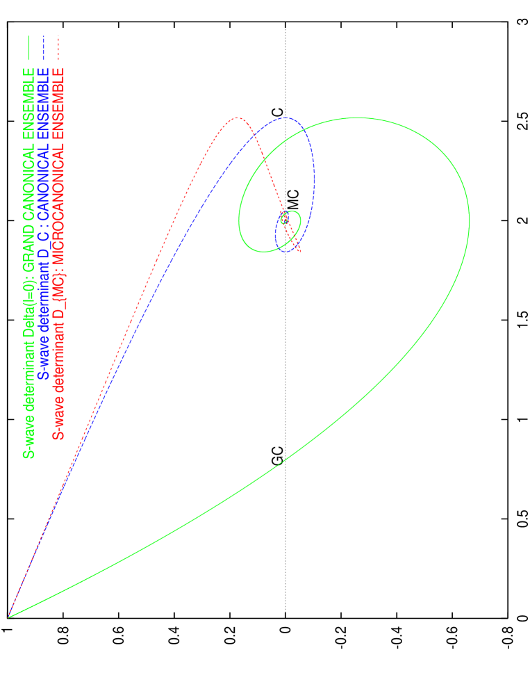
Figure 1: The S-wave determinants $\Delta_{0}(\eta^{R}),\;D_{C}(\eta^{R})$ and $D_{MC}(\eta^{R})$ in the grand canonical, canonical and microcanonical ensembles, respectively, as functions of $\eta^{R}$. Notice that the mean field approximation for each ensemble breaks down as soon as the respective determinant becomes negative when $\eta$ increases starting from $\eta=0$.

3.3 The Microcanonical Ensemble

We have to compute the Gaussian functional integral in eq.(24)

$$\int\int DY\,dy_{0}\;{d{\tilde{\eta}}\over 2\pi i}\;e^{-N\,s^{(2)}_{MC}[Y(.),y_{0},{\tilde{\eta}}]}\;$$ (52)

where $s^{(2)}_{MC}[Y(.),y_{0},{\tilde{\eta}}]$ is given by eq.(25).

As for the canonical ensemble, we start by finding a saddle point ${\tilde{Y}}(.)$ in the Gaussian functional integral (52). We have,

$${{\tilde{Y}}(\vec{x})\over\rho({\vec{x}})}-{\tilde{\eta}}\int d^{3}y\;{{\tilde{Y}}({\vec{y}})+\rho({\vec{y}})\over|{\vec{x}}-{\vec{y}}|}-y_{0}=0\;,$$ (53)

which has as solution

$${\tilde{Y}}(\vec{x})=\rho({\vec{x}})\left[\left(y_{0}+{{\tilde{\eta}}\over\eta_{s}}\right)w(\vec{x})-{{\tilde{\eta}}\over\eta_{s}}\right]\;.$$

Here, $w(\vec{x})$ obeys eq.(43).

We define a new integration variable $Z({\vec{x}})$ in eq.(52) as

$$Y(\vec{x})={\tilde{Y}}(\vec{x})+\rho({\vec{x}})\;Z({\vec{x}})$$

Eq.(52) takes then the form,

$$\int\int DY\,dy_{0}\;{d{\tilde{\eta}}\over 2\pi i}\;e^{-N\,s^{(2)}_{MC}[Y(.),y_{0},{\tilde{\eta}}]} = J\;\int\int DZ\,dy_{0}\;{d{\tilde{\eta}}\over 2\pi i}\;e^{-N\left[A_{0}\,(y_{0})^{2}+B_{0}\,{\tilde{\eta}}^{2}+C_{0}\,{\tilde{\eta}}\,y_{0}+A[Z(.)]\right]}$$ (54)

$$= {\sqrt{3/2}\over\eta\sqrt{\mbox{Det}\left({K_{\rho}\over K_{0}}\right)\,\left[4A_{0}\,B_{0}-C_{0}^{2}\right]}}\;,$$ (56)

where

$$A_{0}\equiv-\frac{1}{2}\int d^{3}x\,\rho({\vec{x}})\;w({\vec{x}})\;,\;B_{0}\equiv{5\over 4\eta^{2}}-{\xi\over\eta}-\frac{1}{2}{\eta^{2}}\int d^{3}x\,\rho({\vec{x}})\;w({\vec{x}})\;,\;C_{0}\equiv\frac{1}{\eta}\left[1-\int d^{3}x\,\rho({\vec{x}})\;w({\vec{x}})\right]$$

$A[Z(.)]$ is given by eq.(44), $J$ by eq.(48) and we have normalized the integral to unit at $\eta=0$.

Then, the argument of the square-root in eq.(56) becomes

$$D_{MC}(\eta^{R})\equiv{2\eta^{2}\over 3}\mbox{Det}\left({K_{\rho}\over K_{0}}\right)\;\left[4A_{0}\,B_{0}-C_{0}^{2}\right]$$ (57)

(58)

$$=\left[6\,f^{2}_{MF}(\eta^{R})-\left(\frac{11}{2}-\eta^{R}\right)f_{MF}(\eta^{R})+\frac{1}{2}\right]\;\prod_{l\geq 1}[\Delta_{l}(\eta^{R})]^{2l+1}\;e^{-\int d^{3}x\;\phi(\vec{x})}\;,$$ (59)

where we used

$$\frac{2}{3}\,(\eta^{R})^{2}\;\Delta_{0}(\eta^{R})\,\left[4A_{0}\,B_{0}-C_{0}^{2}\right]=6\,f^{2}_{MF}(\eta^{R})-\left(\frac{11}{2}-\eta^{R}\right)f_{MF}(\eta^{R})+\frac{1}{2}$$ (60)

All factors in eq.(57) are positive definite except the first one. The sign of $D_{MC}(\eta^{R})$ is therefore determined by the sign of the expression (60).

Thus, $D_{MC}(\eta^{R})$ is positive in the interval $0\leq\eta^{R}\leq\eta^{R}_{C}$ and keeps positive in the second branch of $f_{MF}(\eta^{R})$ for $\eta^{R}_{MC}=2.03085\ldots<\eta^{R}\leq\eta^{R}_{C}$. At the point MC ($\eta^{R}=\eta^{R}_{MC}=2.03085\ldots$ in the second Riemann sheet), the expression (60) becomes negative and the mean field approximation breaks down for the microcanonical ensemble. $D_{MC}(\eta^{R})$ vanishes linearly in $\eta^{R}-\eta^{R}_{MC}$ at $\eta^{R}=\eta^{R}_{MC}$.

In conclusion, the coordinate partition function $w(\xi,N)$ in the microcanonical ensemble takes the form

$$w(\xi,N)\buildrel N>>1\over{=}{e^{-N\,s(\eta^{R})}\over\sqrt{D_{MC}(\eta^{R})}}\left[1+{\cal O}\left({1\over N}\right)\right]$$

Adding the contributions from the functional determinant to the mean field results (10) yields expressions analogous to eqs.(33) but with Det${}_{GC}(\eta^{R})$ replaced by $D_{MC}(\eta^{R})$. That is, in the microcanonical ensemble the function $f(\eta^{R})$ to the order $N^{-1}$ takes the form,

$$f(\eta^{R})=f_{MF}(\eta^{R})+{\eta^{R}\over 6N}{d\over d\eta^{R}}\log D_{MC}(\eta^{R})+{\cal O}\left({1\over N^{2}}\right)\;.$$ (61)

For $\eta^{R}\downarrow\eta^{R}_{MC}$, reaching the point MC, we find

$${\eta^{R}\over 6}\;{d\over d\eta^{R}}\log D_{C}(\eta^{R})\buildrel\eta^{R}\downarrow\eta^{R}_{MC}\over{=}{\eta^{R}_{MC}\over 12(\eta^{R}-\eta^{R}_{MC})}\to+\infty\;,$$

We see that the MF predicts that $pV/[NT]$ grows approaching the critical point MC. This behaviour is confirmed by the Monte Carlo simulations. At the point MC, $pV/[NT]$ increases discontinuously by $50\%$ in the Monte Carlo simulations.

4 Local Physical Magnitudes

We obtain in this section physical magnitudes at at point $\vec{r}$ in the gaseous phase, that is, the space dependence of the particle density, the local energy density, the pressure and the speed of sound. We also compute the average distance between particles.

4.1 Particle Distribution

The particle distribution at thermal equilibrium obtained through the Monte Carlo simulations and mean field methods is inhomogeneous both in the gaseous and condensed phases. In the dilute regime $\eta\ll 1$ the gas density is uniform, as expected.

We plot in figs. 3-6 in paper I the density of particles from Monte Carlo simulations in the cube for the gaseous and for the condensed phases, respectively.

In the mean field approximation and for the spherically symmetric case, the particle density is given by

$$\rho_{MF}(r)=e^{\phi(r)}={\lambda^{2}\;e^{\chi(\lambda r)}\over 4\,\pi\,\eta^{R}}\quad,\quad 0\leq r\leq 1\;.$$ (62)

The mass inside a radius $r$ is then given by

$$M(r)=4\,\pi\int_{0}^{r}{r^{\prime}}^{2}\;\rho_{MF}(r^{\prime})\;dr^{\prime}=-{\lambda\;r^{2}\over\eta^{R}}\,\chi^{\prime}(\lambda r)\;,$$

where we used eq.(4). For small $r$ this gives

$$M(r)\buildrel r\ll 1\over{=}{\lambda^{2}\;r^{3}\over 3\,\eta^{R}}\left[1+{\cal O}(\lambda^{2}\;r^{2})\right]\;.$$ (63)

We find an uniform mass distribution near the origin. This is simply explained by the absence of gravitational forces at $r=0$. Due to the spherically symmetry, the gravitational field exactly vanishes at the origin. The particles exhibit a perfect gas distribution in the vicinity of $r=0$. Actually, eq.(63) is both a short distance and a weak coupling expression. Eq.(63) is valid in the dilute limit $\eta^{R}\ll 1$ for all $0\leq r\leq 1$.

Figure 2: $\log M(r)$ vs. $\log r$ for five different values of $\eta^{R}:\;\eta^{R}_{MC}=2.03085\ldots,\;\eta^{R}_{C}=2.517551\ldots,\;\eta^{R}=2,\;\eta^{R}_{GC}=0.797375\ldots$ and $\eta^{R}=0.1$.

$\eta^{R}$	$\hskip 14.22636ptD$	$\hskip 14.22636ptC$
$0.1$	$2.97$	$1.0$
$\eta^{R}_{GC}=0.797375\ldots$	$2.75$	$1.03$
$2.0$	$2.22$	$1.1$
$\eta^{R}_{C}=2.517551\ldots$	$1.60$	$1.07\hskip 8.5359pt$
$\eta^{R}_{MC}=2.03085\ldots$	$0.98$	$1.11$

TABLE 2. The Fractal Dimension $D$ and the proportionality coefficient $C$ as a function of $\eta^{R}$ from a fit to the mean field results according to ${\cal M}(r)\simeq C\;r^{D}$.

We plot in fig. 2 the particle distribution for $90\%$ of the particles for several values of $\eta^{R}$. We exclude in the plots the region $M(r)<0.1$ where the distribution is uniform.

We find that these mass distributions approximately follow the power law

$${\cal M}(r)\simeq C\;r^{D}$$ (64)

where, as depicted in Table 2, $D$ slowly decreases with $\lambda(\eta^{R})$ from the value $D=3$ for the ideal gas ($\eta=0$) till $D=0.98$ in the extreme limit of the MC point.

The presence of a critical region where scaling holds supports our previous work in the grand canonical ensemble based on field theory[3, 4, 5, 6].

The values of the fractal dimension $D$ of the self-gravitating gas are around $D=2$ (see Table 2). Such value can be analytically obtained assuming exact scale invariance, the virial theorem and the extensivity of the total energy in the limit defined by eq.(1) as follows, [18].

Let us assume that the density scales as $\rho(r)\sim r^{-a}$. Then, using the virial theorem, the total energy $E$ will scale as

$$E\sim\int^{R}d^{3}r\;d^{3}r^{\prime}\;{\rho(r)\;\rho(r^{\prime})\over|{\vec{r}}-{\vec{r}^{\prime}}|}\sim R^{5-2a}$$

Therefore,

$${E\over R^{3}}\sim R^{2(1-a)}$$

Now, extensivity requires $E/V$ to be independent of $R$, that is, $a=1$ and

$$\rho(r)\sim r^{-1}\quad,\quad M(R)\sim R^{2}\;.$$

In addition, this implies that the gravity force in the surface of the gas is independent of $R$.

4.2 Average distance between particles

We investigate here the average distance between particles $<r>$ and the average squared distance $<r^{2}>$. The study of $<r>$ and $<r^{2}>$ as functions of $\eta$ permit a better understanding of the self-gravitating gas and its phase transition in the different statistical ensembles.

These average distances are defined as

$$<r> \equiv \int\int\left|{\vec{r}}-{\vec{r}\,}^{\prime}\right|\;<\rho({\vec{r}})\;\rho({\vec{r}\,}^{\prime})>\;d^{3}r\;d^{3}r^{\prime}\;,$$ (65)

$$<r^{2}> \equiv \int\int\left|{\vec{r}}-{\vec{r}\,}^{\prime}\right|^{2}\;<\rho({\vec{r}})\;\rho({\vec{r}\,}^{\prime})>\;d^{3}r\;d^{3}r^{\prime}$$ (67)

In the mean field approximation we have

$$<\rho({\vec{r}})\;\rho({\vec{r}\,}^{\prime})>=\rho_{MF}({\vec{r}})\;\rho_{MF}({\vec{r}\,}^{\prime})+{\cal O}\left({1\over N}\right)\;.$$ (68)

In addition, in the spherically symmetric case we use eq.(62) for the particle density. In Appendix E we compute the integrals in eqs.(65) and we get as result,

$$<r> = 2-2\;\int_{0}^{1}r^{2}\;dr\;\left[1+{\phi(r)-\phi(1)\over\eta^{R}}\right]^{2}\;,$$ (69)

$$<r^{2}> = 2-{12\over\eta^{R}}\;\int_{0}^{1}r^{2}\;dr\;\left[\phi(r)-\phi(1)\right]$$ (71)

where $\phi(r)$ is given by eq.(3).

We plot $\,<r>$ and $<r^{2}>$ as functions of $\eta^{R}$ in fig. 3. Both $<r>$ and $<r^{2}>$ monotonically decrease with $\lambda(\eta^{R})$. Their values for the ideal gas are

$$\left.<r>\right|_{\eta=0}=\frac{36}{35}=1.02857\ldots\quad,\quad\left.<r^{2}>\right|_{\eta=0}=\frac{6}{5}\;.$$

At the critical points (C for the canonical ensemble and MC for the microcanonical ensemble) the average distances sharply decrease. Both $\,<r>$ and $<r^{2}>$ have infinite slope as functions of $\eta^{R}$ at the point C.

Figure 3: Mean value of the distance between particles ($<r>$) and mean value of the squared distance between particles ($<r^{2}>$) as functions of $\eta^{R}$ in the mean field approach from eqs.(69). Notice that the particles are inside a sphere of unit radius.

We plot in fig. 4 the Monte Carlo results for $<r>$ in a unit cube together with the MF results in a unit sphere. Notice that $<r>$ sharply falls at the point T clearly indicating the transition to collapse.

Figure 4: Mean value of the distance between particles ($<r>$) in a unit cube from Monte Carlo simulations and in a unit sphere from mean field as functions of $\eta^{R}$.

4.3 Local energy density and gravitational potential

The gravitational potential at the point $\vec{q}$ is given by

$$U({\vec{q}})=-G\,m\sum_{1\leq l\leq N}{1\over{|{\vec{q}}-{\vec{q}}_{l}|}}=-{G\,m\over L}\sum_{1\leq l\leq N}{1\over{|{\vec{r}}-{\vec{r}}_{l}|}}$$ (72)

where ${\vec{q}}=L{\vec{r}}$ and ${\vec{q}}_{l}=L{\vec{r}}_{l},1\leq l\leq N.\;U({\vec{q}})$ can be easily related to the saddle point solution in the mean field approach. We write the sum in eq.(72) in terms of the particle density $\rho_{s}({\vec{r}})=e^{\phi({\vec{r}})}$ as,

$$U({\vec{q}})=-{G\,m\,N\over L}\int{d^{3}y\over|{\vec{r}}-{\vec{y}}|}\;\rho({\vec{y}})$$ (73)

Comparison of the saddle point equation (VI.24) in paper I and (73) yields,

$$U({\vec{q}})=-{T\over m}\left[\phi({\vec{r}})-a_{s}\right]$$ (74)

and using eq.(VI.67) in paper I we recover the relation [4]

$$U({\vec{q}})=-{T\over m}\;\Phi_{s}({\vec{r}})\;.$$

The local density of potential energy is thus given by,

$$\epsilon_{P}({\vec{r}})=\frac{1}{2}\;m\;\rho({\vec{q}})\;U({\vec{q}})=-{NT\over 2V}\;\left[\phi({\vec{r}})-a_{s}\right]\;e^{\phi({\vec{r}})}\;,$$

while the local density of kinetic energy takes the form

$$\epsilon_{K}({\vec{r}})={3NT\over 2V}\;e^{\phi({\vec{r}})}\;.$$

It is easy to check that

$$U=\int d^{3}q\;\epsilon_{P}({\vec{r}})\quad,\quad\frac{3}{2}NT=\int d^{3}q\;\epsilon_{K}({\vec{r}})\;.$$

where $U=E-3NT/2$ follows from eq.(10).

In the spherically symmetric case, the local energy density takes the form

$$\epsilon(r)=\epsilon_{K}(r)+\epsilon_{P}(r)={NT\over V}\;{\lambda^{2}\over 8\,\pi\,\eta^{R}}\left[3-\eta^{R}+\chi(\lambda)-\chi(\lambda\,r)\right]\;e^{\chi(\lambda\,r)}\;,$$ (75)

where we used eqs.(3), (6) and eq.(VI.55) from paper I.

The energy density at the surface is always positive:

$$\epsilon(1)={NT\over V}\;{\lambda^{2}\over 8\,\pi\,\eta^{R}}\;(3-\eta^{R})>0\;,$$

whereas the energy density at the center,

$$\epsilon(0)={NT\over V}\;{\lambda^{2}\over 8\,\pi\,\eta^{R}}\left[3-\eta^{R}+\chi(\lambda)\right]\;,$$

is positive for $0\leq\eta^{R}<\eta_{3}^{R}=1.73745\ldots$ and negative beyond the point $\eta^{R}=\eta_{3}^{R}=1.73745\ldots$.

We plot in figs. 5 and 6 the energy density as a function of $r$ for different values of $\eta^{R}$ in the first and second sheets.

Figure 5: The local energy density, $\epsilon(r)$ as a function of $r$ in units of ${NT\over V}$ for $\eta^{R}=0.1,\;1.0,\;1.5$ and $2.0$.

Figure 6: The local energy density, $\epsilon(r)$ as a function of $r$ in units of ${NT\over V}$ for $\eta^{R}$ in the second sheet $\eta^{R}=\eta^{R}_{C},\;2.3,\;2.15$ and $\eta^{R}_{MC}$.

4.4 The pressure at a point ${\vec{r}}$ and the local equation of state

The pressure $p$ that we have obtained in sec. VII [see fig. 9 in paper I] corresponds to the external pressure on the gas. Let us now calculate the local pressure at a point ${\vec{r}}$ in the interior of the self-gravitating gas. We perform that computation in the mean field approach.

The gravitational force is given by

$$F({\vec{q}})=-m\;\rho({\vec{q}})\;{\vec{\nabla}}_{q}U({\vec{q}})={T\,N\over L^{4}}\;e^{\phi({\vec{r}})}\;{\vec{\nabla}}_{r}\phi({\vec{r}})={T\,N\over L^{4}}\;{\vec{\nabla}}_{r}e^{\phi({\vec{r}})}\;,$$ (76)

where we used eq.(74), the expression for the particle density in the volume $L^{3},\;\rho_{V}({\vec{q}})={N\over L^{3}}\;e^{\phi({\vec{r}})}$ and ${\vec{q}}=L\;{\vec{r}}$.

Since the density of force eq.(76) is the gradient of the local pressure, we find

$${\vec{\nabla}}_{r}p({\vec{r}})={T\,N\over L^{3}}\;{\vec{\nabla}}_{r}e^{\phi({\vec{r}})}=T\;{\vec{\nabla}}_{r}\rho_{V}({\vec{r}})$$ (77)

i. e.

$$p({\vec{r}})=T\;\rho_{V}({\vec{r}})$$ (78)

That is, we have shown that the equation of state for the self-gravitating gas is locally the ideal gas equation in the mean field approximation. Notice that contrary to ideal gases, the density here is never uniform in thermal equilibrium. Therefore, in general the pressure at the surface of a given volume is not equal to the temperature times the average density of particles in the volume. In particular, for the whole volume, $PV/[NT]<1$ (except for $\eta=0$).

The local pressure in the spherically symmetric case can be written in a more explicit way using eqs.(3) and (78):

$${p(r)\;V\over N\,T}={\lambda^{2}\over 3\,\eta^{R}}\;e^{\chi(\lambda\,r)}$$ (79)

For $r=1$, eqs. (7) and (10) show that $p=p(1)$ coincides with the external pressure.

The local density and the local pressure monotonically decreases with $r$.

The particle density at the origin follows from eqs.(62) and (4):

$$\rho(r=0)={\lambda^{2}\over 4\,\pi\;\eta^{R}}$$ (80)

This particle density at the origin grows when moving from $\eta=0$ to MC as shown in fig. 7. In particular, for $\eta^{R}=0$ we have

$$\left.\rho(r=0)\right|_{\eta^{R}=0}={3\over 4\pi}$$ (81)

where we used eqs. (7), (9) and (80). Notice that $\rho(r)$ is $r$-independent for $\eta^{R}=0$.

The particle density at the surface is proportional to $f_{MF}(\eta^{R})$ [see eq.(6)] and plotted in fig. 9 of paper I. We see that it decreases when moving from $\eta=0$ to $\eta=\eta_{Min}=2.20731\ldots$ in the second sheet. The migration of particles towards the center as $\eta$ varies is manifestly responsible for these variations in the density.

Figure 7: $\rho(r=0)={\lambda^{2}\over 4\,\pi\;\eta^{R}}$ as a function of $\eta^{R}$. For $\eta^{R}=0$, $\rho(r=0)=3/(4\pi)$ [see eq.(81)].

The pressure (and density) contrast is given by

$${p(0)\over p(1)}={\rho(0)\over\rho(1)}=e^{-\chi(\lambda)}$$

We plot in fig. 8 $\chi(\lambda(\eta^{R}))$ as a function of $\eta^{R}$. For $\eta^{R}=\eta^{R}_{C}$ and $\eta^{R}=\eta^{R}_{MC}$ we recover the known values $p(0)/p(1)=32.125\ldots$ and $p(0)/p(1)=708.63\ldots$, respectively [14, 15].

Figure 8: $\chi(\lambda(\eta^{R}))=\log{p(0)\over p(1)}=\log{\rho(0)\over\rho(1)}$ as a function of $\eta^{R}$.

Notice that $pV/[NT]<1$ (see fig. 9 in paper I) for $\eta>0$ although the equation of state is locally the one of an ideal gas as we have showed. The inhomogeneous particle distribution in the self-gravitating gas is responsible of such inequality.

Local equations of state other than the ideal gas are often assumed in the context of self-gravitating fluids [8, 9, 11, 14]. Our result imply that forces other than gravitational are necessary to obtain a non-ideal local equation of state in thermal equilibrium.

We have thus shown the equivalence for the self-gravitating gas between the statistical mechanical treatment in the mean field approach with the hydrostatic description [9]-[16].

4.5 The speed of sound as a function of ${\vec{r}}$

For very short wavelengths $\lambda_{s}\ll L$, the sound waves just feel the local equation of state (78) and the speed of sound will be that of an ideal gas. For long wavelengths (of the order $L$), the situation changes. The calculation in eq.(16) corresponds to the speed of sound for an external wave arriving on the sphere in the long wavelength limit. Let us now make the analogous calculation for a wave reaching the point ${\vec{q}}$ inside the gas.

Our starting point is again eq.(III.29) in paper I,

$$v_{s}^{2}({\vec{q}})=-{{c_{P}\;V^{2}}\over{c_{V}\;N}}\left({\partial p({\vec{q}})\over\partial V}\right)_{T,{\vec{q}}}\;,$$ (82)

where $c_{P}$ and $c_{V}$ are the specific heats of the whole system at constant (external) pressure and volume, respectively, and $p({\vec{q}})$ is the local pressure at the point ${\vec{q}}$.

We find for the spherically symmetrical case in MF

$${v_{s}^{2}(r)\over T}={c_{P}\over c_{V}}\;{\lambda^{2}\over 9\,\eta^{R}\;\left[3f(\eta^{R})-1\right]}\;\left[6\,f(\eta^{R})+\lambda\,r\;\chi^{\prime}(\lambda\,r)\right]\;e^{\chi(\lambda\,r)}\;,$$ (83)

where we used eqs.(79), (82) and

$$\left({\partial\eta\over\partial V}\right)_{T}=-{\eta\over 3\,V}\;.$$

[$\lambda$ is a function of $\eta^{R}$ as defined by eq.(5)].

At the surface, $(r=1),\;v_{s}^{2}(r)$ reduces to eq.(16) after using eqs.(5), (7), (17) and (18).

Figure 9: $v_{s}^{2}(r)/v_{s}^{2}(1)$ as a function of $r$ for $\eta^{R}=2.0,\;1.5,\;1.0$ and $0.1$. That is, values of $\eta^{R}$ smaller than $\eta^{R}_{0}=2.43450\ldots$. $v_{s}^{2}(r)/v_{s}^{2}(1)$ is here always positive and decreases with $r$.

Figure 10: $v_{s}^{2}(r)/v_{s}^{2}(1)$ as a function of $r$ for values of $\eta^{R}$ around $\eta^{R}_{0}=2.43450\ldots$. Positive values of $v_{s}^{2}(r)/v_{s}^{2}(1)$ correspond to $\eta^{R}<\eta^{R}_{0}$ and negative values of $v_{s}^{2}(r)/v_{s}^{2}(1)$ correspond to $\eta^{R}>\eta^{R}_{0}$. We see that the speed of sound squared tends to $+\infty$ in the bulk ($r<1$) for $\eta^{R}\uparrow\eta^{R}_{0}$ while it tends to $-\infty$ for $\eta^{R}\downarrow\eta^{R}_{0}$.

Figure 11: $v_{s}^{2}(r)/v_{s}^{2}(1)$ as a function of $r$ for $\eta^{R}$ in the second sheet: $\eta^{R}=\eta^{R}_{MC}=2.03085\ldots,\;2.15,\;2.3$ and $\eta^{R}_{C}=2.517551\ldots$. $v_{s}^{2}(r)/v_{s}^{2}(1)$ is here strongly negative in the core of the sphere. Notice that $v_{s}^{2}(1)<0$ for $\eta^{R}=\eta^{R}_{MC}=2.03085\ldots$ while $v_{s}^{2}(1)>0$ for $\eta^{R}=2.15,\;2.3$ and $\eta^{R}_{C}$.

For $\eta^{R}<\eta^{R}_{0}=2.43450\ldots$ in the first sheet, $v_{s}^{2}(r)$ is positive and decreases with $r$ as shown in fig. 9.

At $\eta^{R}=\eta^{R}_{0},\;v_{s}^{2}(r)$ diverges for all $0\leq r<1$ due to the factor $c_{P}$ in eq.(83) [cfr. eq.(18)]. The derivative of $p$ with respect to $V$ is proportional to $6\,f(\eta^{R})+\lambda\,r\;\chi^{\prime}(\lambda\,r)$ as we see in eq.(83). At $r=1$ this factor becomes $6\,f(\eta^{R})-\eta^{R}$ [see eq.(5)] which exactly vanishes at $\eta^{R}=\eta^{R}_{0}$ canceling the singularity that $c_{P}$ possesses at such point [see eq.(18)]. Thus, $v_{s}^{2}(1)$ is regular at $\eta^{R}=\eta^{R}_{0}$.

$v_{s}^{2}(r)$ becomes large and positive below and near $\eta^{R}_{0}$ and large and negative above and near $\eta^{R}_{0}=2.43450\ldots$ as depicted in fig. 10. This singular behaviour witness the appearance of strong instabilities at $\eta^{R}=\eta^{R}_{0}$. For $\eta^{R}>\eta^{R}_{0},\;v_{s}(r)$ becomes imaginary indicating the exponential growth of disturbances in the gas. This phenomenon is especially dramatic in the denser regions (the core).

For $\eta^{R}$ beyond $\eta^{R}_{0}$ and before $\eta^{R}_{1}=2.14675\ldots$ in the second sheet $v_{s}^{2}(r)$ stays negative around the core while it becomes positive in the external regions as depicted in fig. 11. For example, $v_{s}^{2}(r)$ is positive at $\eta^{R}=\eta^{R}_{C}$ for $r>0.4526\ldots$.

For $\eta^{R}$ in the second sheet beyond $\eta^{R}_{1}$ and before $\eta^{R}_{MC},\;v_{s}^{2}(r)$ is positive in the core and negative outside.

5 $\nu$-dimensional generalization

The self-gravitating gas can be studied in $\nu$-dimensional space where the Hamiltonian takes the form

$$H_{N}=\sum_{l=1}^{N}\;{{p_{l}^{2}}\over{2m}}-G\,m^{2}\sum_{1\leq l<j\leq N}{1\over{|{\vec{q}}_{l}-{\vec{q}}_{j}|_{A}^{\nu-2}}},\quad{\rm for}\;\nu\neq 2$$ (84)

and

$$H_{N}=\sum_{l=1}^{N}\;{{p_{l}^{2}}\over{2m}}-G\,m^{2}\sum_{1\leq l<j\leq N}\log{1\over{|{\vec{q}}_{l}-{\vec{q}}_{j}|_{A}}},\quad{\rm at}\;\nu=2\;.$$ (85)

The partition function in the microcanonical, canonical and grand canonical ensembles takes forms analogous to eqs.(II.2), (III.1) and (VI.7) in paper I, respectively.

We now find for the microcanonical ensemble,

$$S(E,N)=\log\left[{N^{\nu N-2}\,m^{3\nu N/2-2}\,L^{\nu(2-\nu/2)N+\nu-2}\,G^{\nu N/2-1}\over N!\,\Gamma\left({\nu N\over 2}\right)\,{(2\pi)}^{\nu N/2}}\right]+\log w(\xi,N)\;.$$

where the coordinate partition function takes now the form

$$w(\xi,N)\equiv\int_{0}^{1}\ldots\int_{0}^{1}\prod_{l=1}^{N}\;d^{\nu}r_{l}\;\left[\xi+{1\over N}u({\vec{r}}_{1},\ldots,{\vec{r}}_{N})\right]^{\nu N/2-1}\theta\left[\xi+{1\over N}u({\vec{r}}_{1},\ldots,{\vec{r}}_{N})\right]\;.$$

with

$$\xi={E\,L^{\nu-2}\over G\,m^{2}\,N^{2}}$$ (86)

and

$$u({\vec{r}}_{1},\ldots,{\vec{r}}_{N})\equiv{1\over N}\sum_{1\leq l<j\leq N}{1\over{|{\vec{r}}_{l}-{\vec{r}}_{j}|_{a}^{\nu-2}}}\;.$$

In the canonical ensemble we obtain now,

$${\cal Z}_{C}(N,T)={1\over N!}\left({mTL^{2}\over{2\pi}}\right)^{\frac{\nu N}{2}}\;\int_{0}^{1}\ldots\int_{0}^{1}\prod_{l=1}^{N}d^{\nu}r_{l}\;\;e^{\eta\;u({\vec{r}}_{1},\ldots,{\vec{r}}_{N})}$$

where the variable $\eta$ takes the form

$$\eta={G\,m^{2}N\over L^{\nu-2}\;T}\;.$$ (87)

As we can see from eqs.(86)-(87) the only change going off three dimensional space is in the exponent of $L$.

In $\nu$-dimensional space the thermodynamic limit is defined as $V,\;N\to\infty$ keeping $\eta$ and $\xi$ fixed. That is, $N/L^{\nu-2}=N/V^{1-2/\nu}$ is kept fixed. The volume density of particles $N/V$ vanishes as $V^{-2/\nu}$ for $V,\;N\to\infty$ and $\nu>2$. It is a dilute limit for $\nu>2$.

When $\nu\leq 2$, one has to assume that the temperature tends to infinity in the thermodynamic limit in order to keep $\eta$ and $\xi$ fixed as $V,\;N\to\infty$.

6 The Interstellar Medium

The interstellar medium (ISM) is a gas essentially formed by atomic (HI) and molecular ($H_{2}$) hydrogen, distributed in cold ($T\sim 5-50K$) clouds, in a very inhomogeneous and fragmented structure. These clouds are confined in the galactic plane and in particular along the spiral arms. They are distributed in a hierarchy of structures, of observed masses from $10^{-2}\;M_{\odot}$ to $10^{6}M_{\odot}$. The morphology and kinematics of these structures are traced by radio astronomical observations of the HI hyper fine line at the wavelength of 21cm, and of the rotational lines of the CO molecule (the fundamental line being at 2.6mm in wavelength), and many other less abundant molecules. Structures have been measured directly in emission from 0.01pc to 100pc, and there is some evidence in VLBI (very long based interferometry) HI absorption of structures as low as $10^{-4}\;pc=20$ AU (3 $10^{14}\;cm$). The mean density of structures is roughly inversely proportional to their sizes, and vary between $10$ and $10^{5}\;atoms/cm^{3}$ (significantly above the mean density of the ISM which is about $0.1\;atoms/cm^{3}$ or $1.6\;10^{-25}\;g/cm^{3}$ ). Observations of the ISM revealed remarkable relations between the mass, the radius and velocity dispersion of the various regions, as first noticed by Larson [21], and since then confirmed by many other independent observations (see for example ref.[22]). From a compilation of well established samples of data for many different types of molecular clouds of maximum linear dimension (size) $R$, total mass $M$ and internal velocity dispersion $\Delta v$ in each region:

$$M(R)\sim R^{d_{H}}\quad,\quad\Delta v\sim R^{q}\;,$$ (88)

over a large range of cloud sizes, with $10^{-4}\;-\;10^{-2}\;pc\;\leq R\leq 100\;pc,\;$

$$1.4\leq d_{H}\leq 2,\;0.3\leq q\leq 0.6\;.$$ (89)

These scaling relations indicate a hierarchical structure for the molecular clouds which is independent of the scale over the above cited range; above $100$ pc in size, corresponding to giant molecular clouds, larger structures will be destroyed by galactic shear.

These relations appear to be universal, the exponents $d_{H},\;q$ are almost constant over all scales of the Galaxy, and whatever be the observed molecule or element. These properties of interstellar cold gas are supported first at all from observations (and for many different tracers of cloud structures: dark globules using ¹³CO, since the more abundant isotopic species ¹²CO is highly optically thick, dark cloud cores using $HCN$ or $CS$ as density tracers, giant molecular clouds using ¹²CO, HI to trace more diffuse gas, and even cold dust emission in the far-infrared). Nearby molecular clouds are observed to be fragmented and self-similar in projection over a range of scales and densities of at least $10^{4}$, and perhaps up to $10^{6}$.

The physical origin as well as the interpretation of the scaling relations (88) have been the subject of many proposals. It is not our aim here to account for all the proposed models of the ISM and we refer the reader to refs.[22] for a review.

The physics of the ISM is complex, especially when we consider the violent perturbations brought by star formation. Energy is then poured into the ISM either mechanically through supernovae explosions, stellar winds, bipolar gas flows, etc.. or radiatively through star light, heating or ionizing the medium, directly or through heated dust. Relative velocities between the various fragments of the ISM exceed their internal thermal speeds, shock fronts develop and are highly dissipative; radiative cooling is very efficient, so that globally the ISM might be considered isothermal on large-scales. Whatever the diversity of the processes, the universality of the scaling relations suggests a common mechanism underlying the physics.

We proposed that self-gravity is the main force at the origin of the structures, that can be perturbed locally by heating sources[3, 4]. Observations are compatible with virialised structures at all scales. Moreover, it has been suggested that the molecular clouds ensemble is in isothermal equilibrium with the cosmic background radiation at $T\sim 3K$ in the outer parts of galaxies, devoid of any star and heating sources [7]. This colder isothermal medium might represent the ideal frame to understand the role of self-gravity in shaping the hierarchical structures.

In order to compare the properties of the self-gravitating gas with the ISM it is convenient to express $m,\;T$ and $L$ in $\eta$ in appropriate units. We find from eq.(2)

$$\eta=0.52193\;{m\;{\cal M}_{\odot}\over L\;T}\;,$$

where $m$ is in multiples of the hydrogen atom mass, $T$ in Kelvin, $L$ in parsecs and ${\cal M}_{\odot}$ is the mass of the cloud in units of solar masses. Notice that $L$ is many times ($\sim 10$) the size of the cloud.

The observed parameters of the ISM clouds[22] yield an $\eta$ around $\sim 2.0$ for clouds not too large: ${\cal M}_{\odot}<1000$. Such $\eta$ is in the range where the self-gravitating gas exhibits scaling behaviour.

We conclude that the self-gravitating gas in thermal equilibrium well describe the observed fractal structures and the scaling relations in the ISM clouds [see, for example fig. 2 and table 2]. Hence, self-gravity accounts for the structures in the ISM.

7 Discussion

We have presented in paper I and here a set of new results for the self-gravitating thermal gas obtained by Monte Carlo and analytic methods. They provide a complete picture for the thermal self-gravitating gas.

Starting from the partition function of the self-gravitating gas, we have proved from a microscopic calculation that the local equation of state $p(\vec{r})=T\;\rho_{V}(\vec{r})$ and the hydrostatic description are exact. Indeed, the dilute nature of the thermodynamic limit ($N\sim L\to\infty$ with $N/L$ fixed) together with the long range nature of the gravitational forces play a crucial role in the obtention of such ideal gas equation of state.

More generally, one can investigate whether a hydrodynamical description will apply for a self-gravitating gas. One has then to estimate the mean free path $(l)$ for the particles and compare it with the relevant scales $a$ in the system [19]. We have,

$$l\sim{1\over\rho_{V}\;\sigma_{t}}\sim{L^{3}\over N\;\sigma_{t}}$$ (90)

where $\rho_{V}={N\over L^{3}}\;\rho$ is the volume density of particles and $\sigma_{t}$ the total transport cross section.

Due to the long range nature of the gravitational force, $\sigma_{t}$ diverges logarithmically for small angles. On a finite volume the impact parameter is bounded by $L$ and the smaller scattering angle is of the order of

$${\Delta q\over q}\sim{G\;m^{2}\over L\,T}$$

since $q=mv\sim\sqrt{m\;T}$ and $\Delta q\sim{G\,m^{2}\over L^{2}}{L\over v}\sim{G\,m^{5/2}\over L\,\sqrt{T}}$.

We then have for the transport cross section[19],

$$\sigma_{t}\sim{(G\,m)^{2}\over|\vec{v}-\vec{v}^{\prime}|^{4}}\log{L\,T\over G\,m^{2}}\sim\left({L\,N\over\eta}\right)^{2}\log{N\over\eta}$$ (91)

where we used that $v\sim\sqrt{T\over m}$ and $|\vec{v}-\vec{v}^{\prime}|\sim\Delta q/m$. As we see, the collisions with very large impact parameters ($\sim L$) dominate the cross-section.

From eqs.(90) and (91), we find for the mean free path:

$$l\sim{L\over N}\;\left({G\,m^{2}\over T\,L}\right)^{2}{1\over\log{T\,L\over G\,m^{2}}}\sim{L\over N^{3}}{\eta^{2}\over\log{N\over\eta}}\;,$$ (92)

where we have here replaced $\rho_{V}$ by ${N\over L^{3}}$. A more accurate estimate introduces the factor $\rho=e^{\phi}$ in the denominator of $l$. This factor for spherical symmetry can vary up to two orders of magnitude [see fig. 7] but it does not change essentially the estimate (92).

We see from eq.(92) that in the thermodynamic limit $l$ becomes extremely small compared with any length $a={\cal O}(N^{0})$ that stays fixed for $N\to\infty$. We find from eq.(92),

$${l\over a}\sim{1\over N^{2}}{\eta^{2}\over\log{N\over\eta}}\;,$$

In conclusion, the smallness of the ratio $l/a$ (Knudsen number) guarantees that the hydrodynamical description for a self-gravitating fluid becomes exact in the $N,\;L\to\infty$ limit for all scales ranging from the order $L^{0}$ till the order $L$.

It must me noticed that the time between two collisions $t_{col}=l/v\sim l\,\sqrt{m\over T}$ is different both from the relaxation time and from the crossing time used in the literature. In particular, it is well known that[9, 16]

$${t_{crossing}\over t_{relaxation}}\sim{8\over N}\,\log N\;.$$

This formula does not concern the time $t_{col}$ between two successive collisions. The time $t_{col}$ is indeed very short due to the small angle behaviour of the gravitational cross section. For constant cross sections one finds a very different result for $t_{col}$ [see ref. [16]].

In this paper and in its companion paper [1] we thoroughly investigate the physics of the self-gravitating gas in thermal equilibrium. It is natural to study now the hydrodynamics of the self-gravitating fluid using $p(\vec{r})=T\;\rho(\vec{r})$ as local equation of state. A first work on this direction is ref.[23].

8 Acknowledgements

One of us (H J de V) thanks M. Picco for useful discussions on Monte Carlo methods. We thank S. Bouquet for useful discussions.

Appendix A Calculation of Functional Determinants in the Spherically Symmetric Case

We compute here the determinant of the one-dimensional differential operator:

$$D_{1}(l)=-{d^{2}\over dr^{2}}-\frac{2}{r}{d\over dr}+{l(l+1)\over r^{2}}-4\pi\eta^{R}\;e^{\phi(r)}$$

where $\phi(r)$ is the stationary point given by eqs.(3)-(4).

It is convenient to change the variable $r$ to

$$x\equiv\log r\quad,\quad 0\leq r\leq 1\quad,\quad-\infty\leq x\leq 0\;,$$

and perform a similarity transformation by $\sqrt{r}=e^{x/2}$ on $D_{1}(l)$. That is, we define

$$D(l)\equiv e^{-x/2}\;D_{1}(l)\;e^{x/2}=-{d^{2}\over dx^{2}}-k^{2}+v(x)\;,$$

where,

$$v(x)\equiv-4\pi\eta^{R}\;e^{\phi(r=e^{x})+2x}\quad,\quad k\equiv i\left(l+\frac{1}{2}\right)\;.$$

$D(l)$ has the form of a standard Schrödinger operator. Notice that,

$$\lim_{x\to-\infty}v(x)=0\quad\mbox{and}\quad v(0)=-3\,\eta^{R}\,f_{MF}(\eta^{R})<0\;.$$

We thus have an ‘attractive’ potential $v(x)$. The appearance of a ‘bound state’ (that is, a negative eigenvalue $k^{2}<0$) corresponds here to an instability in the self-gravitating gas.

We compute now the determinant

$$\Delta_{l}\equiv\Delta(k)\equiv{\mbox{Det}\left[-{d^{2}\over dx^{2}}-k^{2}+v(x)\right]\over\mbox{Det}\left[-{d^{2}\over dx^{2}}-k^{2}\right]}$$

where we normalize at $v=0$, as usual.

The logarithmic derivative with respect to $k^{2}$ can be expressed in terms of the inverse of the operator $D(l)$

$$-{\partial\log\Delta(k)\over\partial k^{2}}=\int_{-\infty}^{0}dx\left[\left(x\right|{1\over-{d^{2}\over dx^{2}}-k^{2}+v(x)}\left|x\right)-\left(x\right|{1\over-{d^{2}\over dx^{2}}-k^{2}}\left|x\right)\right]\;.$$ (93)

In order to express the Green function (inverse of the operator $D(l)$) we introduce the Jost and regular solutions of the Schrödinger-like equation

$$\left[-{d^{2}\over dx^{2}}-k^{2}+v(x)\right]f(k,x)=0\;.$$ (94)

The solution of eq.(94) with the asymptotic behaviour

$$f(k,x)\buildrel x\to-\infty\over{=}e^{-ikx}=e^{\left(l+\frac{1}{2}\right)x}\buildrel r\to 0\over{=}r^{l+\frac{1}{2}}\;.$$ (95)

is called the Jost solution, while the solutions $\varphi(k,x)$ of eq.(94) obeying the boundary conditions

$$\varphi(k,0)=\alpha\quad,\quad{\dot{\varphi}}(k,0)=\beta$$ (96)

where $\alpha$ and $\beta$ are $k$-independent arbitrary parameters, are called regular solutions. The values of $\alpha$ and $\beta$ must be selected on physical grounds as discussed in sec. III. $\Delta(k)$ explicitly depends on them as we shall see below.

For large and negative $x$ we have

$$\varphi(k,x)\buildrel x\to-\infty\over{=}F(k)\;e^{ikx}+G(k)\;e^{-ikx}$$

where the coefficients $F(k)$ and $G(k)$ depend on $v(.)$. $F(k)$ is called the Jost function.

The small fluctuations defined by eq.(29) are related to the regular solutions by

$$y_{l}(r)={1\over\sqrt{r}}\;\varphi(k=i\left(l+\frac{1}{2}\right),\,x=\log r)$$ (97)

where $y_{l}(r)$ is the radial part of $Y(\vec{x})$ in the $l$th. wave [see eq.(29)].

The Green function of $D(l)$ takes then the form

$$\left(x\right|{1\over-{d^{2}\over dx^{2}}-k^{2}+v(x)}\left|x^{\prime}\right)={i\over 2\,k}\;\varphi(k,x_{>})\;f(k,x_{<})\;,$$ (98)

where $x_{>}$ ($x_{<}$) stands for the larger (the smaller) between $x$ and $x^{\prime}$.

Inserting eq.(98) into eq.(93), the integration over $x$ can be performed with the help of wronskian identities with the result

$$\Delta(k)={2\,k\;F(k)\over\alpha\;k-i\;\beta}\;,$$

where we used that $\Delta(\infty)=1$ as normalization.

The Jost function $F(k)$ can be expressed in terms of the Jost solution at the origin just computing at the origin the wronskian of the regular and Jost solutions,

$$F(k)={1\over 2\,i\,k}\left[\beta f(k,0)-\alpha{\dot{f}}(k,0)\right]\;.$$

Therefore, once the Jost solution is known, the calculation of the determinant is immediate

$$\Delta(k)={\beta f(k,0)-\alpha{\dot{f}}(k,0)\over\beta+i\,\alpha\;k}$$ (99)

Notice that $\Delta(k)$ is an homogeneous function of $\alpha$ and $\beta$.

We impose the physical boundary conditions (30) to the regular solution (96). This gives

$$(2\,l+1)\alpha+2\,\beta=0$$ (100)

and

$$\Delta_{l}=\frac{1}{2}f(k,0)+{1\over 2l+1}{\dot{f}}(k,0)$$ (101)

Figure 12: The partial wave determinants for $l=1,\,2,\,3$ and $4$ as a function of $\eta^{R}$. Notice that all these determinants are positive definite for $\eta^{R}_{C}\geq\eta^{R}\geq 0$.

A.1 The S-wave determinant

For $l=0,\;k=i/2$, eq.(94) can be solved in terms of the stationary point solution $\phi(r=e^{x})$. That is,

$$f(i/2,x)=e^{x/2}\left[1+\frac{1}{2}\;{d\phi(r=e^{x})\over dx}\right]\;,$$ (102)

obeys both eq.(94) and the boundary conditions (95). Eq.(94) for the function (102) can be checked just taking the derivative of the stationary point equation (VI.43) in paper I with respect to $x=\log r$.

We can now compute $f(i/2,0)$ and ${\dot{f}}(i/2,0)$ using eqs.(VI.43), (VI.46) in paper I, and (6) with the result,

$$f(i/2,0)=1-{\eta^{R}\over 2}\quad,\quad{\dot{f}}(i/2,0)=\frac{1}{2}+{\eta^{R}\over 4}-\frac{3}{2}\;\eta^{R}\;f_{MF}(\eta^{R})\;.$$

This yields for the S-wave determinant (99)

$$\Delta_{0}=\Delta(k=i/2)={1\over\alpha-2\,\beta}\,\left\{\alpha\left[1+{\eta^{R}\over 2}-3\,\eta^{R}\;f_{MF}(\eta^{R})\right]+\beta\;(\eta^{R}-2)\right\}$$

for arbitrary values of $\alpha$ and $\beta$.

For the boundary conditions (100) we find

$$\Delta_{0}(\eta^{R})=1-\frac{3}{2}\,\eta^{R}\,f_{MF}(\eta^{R})\;.$$ (103)

A.2 The P-wave determinant

For $l=1,\;k=3i/2$, eq.(94) can also be solved in terms of the stationary point solution $\phi(r=e^{x})$. That is,

$$f(3i/2,x)=-{3\over\lambda^{2}}\;e^{-x/2}\;{d\phi(r=e^{x})\over dx}$$ (104)

obeys both eq.(94) and the boundary conditions (95). Eq.(94) for the function (104) can be checked just taking the derivative with respect to $r$ of the stationary point equation (VI.43) in paper I.

We obtain for $f(3i/2,0)$ and ${\dot{f}}(3i/2,0)$,

$$f(3i/2,0)={3\,\eta^{R}\over\lambda^{2}}\quad,\quad{\dot{f}}(3i/2,0)={9\over\lambda^{2}}\left[f_{MF}(\eta^{R})-{\eta^{R}\over 2}\right]$$

where we used again eqs.(VI.43), (VI.46) in paper I, and (6).

We finally obtain for the P-wave determinant for arbitrary values of $\alpha$ and $\beta$,

$$\Delta_{1}=\Delta(k=3i/2)={3\,\eta^{R}\over\lambda^{2}(3\,\alpha-2\,\beta)}\left\{3\,\alpha\left[2\,f_{MF}(\eta^{R})-1\right]-2\,\beta\right\}$$

For the boundary conditions (100) we find

$$\Delta_{1}(\eta^{R})={3\,\eta^{R}\over\lambda^{2}}f_{MF}(\eta^{R})\;.$$ (105)

A.3 The D-wave and higher waves

We plot in fig. 12 the determinants for $l=2,3,4$ and $5$ for the boundary conditions (100) We see that these partial waves determinants are positive for all positive values of $\eta^{R}\leq\eta^{R}_{C}$.

We can evaluate the Jost solutions asymptotically for large $k$ (large $l$). Using the standard Riccati transformations yields

$$f(k,x)=e^{(l+\frac{1}{2})x}\left[1+{I(x)\over 2l+1}-{I^{2}(x)+2\,v(x)\over 2(2l+1)^{2}}+{\cal O}\left({1\over(2l+1)^{3}}\right)\right]$$

where $k=i\left(l+\frac{1}{2}\right)$ and

$$I(x)\equiv\int_{-\infty}^{x}dy\,v(y)=\lambda\,e^{x}\,\chi^{\prime}(\lambda e^{x})+\chi(\lambda e^{x})$$

Therefore, for the boundary conditions (100) we find from eq.(101),

$$\Delta_{l}(\eta^{R})=1+{I(0)\over 2l+1}-{I^{2}(0)\over 2(2l+1)^{2}}+{\cal O}\left({1\over(2l+1)^{3}}\right)$$

where,

$$I(0)=\log\left[{3\,\eta^{R}\over\lambda^{2}}f_{MF}(\eta^{R})\right]-\eta^{R}\;.$$

Appendix B Calculation of $<r>$ and $<r^{2}>$ in the mean field

In the mean field approach we have from eqs.(65) and (68)

$$<r>=\int_{0}^{1}r^{2}\;dr\int_{0}^{1}{r^{\prime}}^{2}\;dr^{\prime}\;\int d\Omega(\hat{r})\;\int d\Omega(\hat{r}^{\prime})\;\rho(r)\;\rho(r^{\prime})\;\sqrt{r^{2}+{r^{\prime}}^{2}-2rr^{\prime}\;\cos({\hat{r},\hat{r}^{\prime}})}\;,$$

$$<r^{2}>=\int_{0}^{1}r^{2}\;dr\int_{0}^{1}{r^{\prime}}^{2}\;dr^{\prime}\;\int d\Omega(\hat{r})\;\int d\Omega(\hat{r}^{\prime})\;\rho(r)\;\rho(r^{\prime})\;[r^{2}+{r^{\prime}}^{2}-2rr^{\prime}\;\cos({\hat{r},\hat{r}^{\prime}})]\;.$$

Integrating over the angles yield,

$$<r>={16\,\pi^{2}\over 3}\int_{0}^{1}r\,dr\;\rho(r)\left\{\int_{0}^{r}{r^{\prime}}^{2}\;dr^{\prime}\;\rho(r^{\prime})\left[{r^{\prime}}^{2}+3\,r^{2}\right]+r\;\int_{r}^{1}r^{\prime}\;dr^{\prime}\;\rho(r^{\prime})\left[r^{2}+3\,{r^{\prime}}^{2}\right]\right\}$$

$$<r^{2}>=8\pi\;\int_{0}^{1}r^{4}\;dr\;\rho(r)$$

We have then to compute integrals of the type $\int r^{n}\;dr\;e^{\phi(r)}\;$ for $n=1,\;2,\;3$ and $4$. We find using eqs.(VI.43), (VI.45), (VI.46) and (VI.54) in paper I,

$$4\,\pi\,\eta^{R}\int_{0}^{r}{r^{\prime}}^{2}\;e^{\phi(r^{\prime})}\;dr^{\prime} = -r^{2}\;{d\phi(r)\over dr}$$ (106)

$$4\,\pi\,\eta^{R}\int_{r}^{1}r^{\prime}\;e^{\phi(r^{\prime})}\;dr^{\prime} = {d\over dr}[r\;\phi(r)]+\eta^{R}-\phi(1)$$ (108)

$$4\,\pi\,\eta^{R}\int_{r}^{1}{r^{\prime}}^{3}\;e^{\phi(r^{\prime})}\;dr^{\prime} = r^{3}\,{d\phi(r)\over dr}-r^{2}\phi(r)+\eta^{R}+\phi(1)-2\int_{r}^{1}r^{\prime}\;\phi(r^{\prime})\;dr^{\prime}$$ (110)

$$4\,\pi\,\eta^{R}\int_{0}^{r}{r^{\prime}}^{4}\;e^{\phi(r^{\prime})}\;dr^{\prime} = -r^{4}\,{d\phi(r)\over dr}+2\,r^{3}\phi(r)-6\,\int_{0}^{r}{r^{\prime}}^{2}\;\phi(r^{\prime})\;dr^{\prime}$$ (112)

Collecting all terms yields after calculation eq.(69).

References

- [1] H. J. de Vega, N. Sánchez, ‘Statistical Mechanics of the Self-Gravitating Gas and Fractal Structures. I’, astro-ph/0101568. Quoted as paper I in the text.
- [2] L. D. Landau and E. M. Lifchitz, Physique Statistique, 4ème édition, Mir-Ellipses, 1996.
- [3] H. J. de Vega, N. Sánchez and F. Combes, Nature, 383, 56 (1996).
- [4] H. J. de Vega, N. Sánchez and F. Combes, Phys. Rev. D54, 6008 (1996).
- [5] H. J. de Vega, N. Sánchez and F. Combes, Ap. J. 500, 8 (1998).
- [6] H. J. de Vega, N. Sánchez and F. Combes, in ‘Current Topics in Astrofundamental Physics: Primordial Cosmology’, NATO ASI at Erice, N. Sánchez and A. Zichichi editors, vol 511, Kluwer, 1998.
- [7] D. Pfenniger, F. Combes, L. Martinet, A&A 285, 79 (1994) D. Pfenniger, F. Combes, A&A 285, 94 (1994)
- [8] S. Chandrasekhar, ‘An Introduction to the Study of Stellar Structure’, Chicago Univ. Press, 1939.
- [9] See for example, W. C. Saslaw, ‘Gravitational Physics of stellar and galactic systems’, Cambridge Univ. Press, 1987.
- [10] R. Emden, Gaskugeln, Teubner, Leipzig und Berlin, 1907.
- [11] D. Lynden-Bell and R. M. Lynden-Bell, Mon. Not. R. astr. Soc. 181, 405 (1977). D. Lynden-Bell, cond-mat/9812172.
- [12] D. Lynden-Bell and R. Wood, Mon. Not. R. astr. Soc. 138, 495 (1968).
- [13] V. A. Antonov, Vest. Leningrad Univ. 7, 135 (1962).
- [14] T. Padmanabhan, Phys. Rep. 188, 285 (1990).
- [15] G. Horwitz and J. Katz, Ap. J. 211, 226 (1977) and 222, 941 (1978).
- [16] J. Binney and S. Tremaine, Galactic Dynamics, Princeton Univ. Press.
- [17] J. Avan and H. J. de Vega, Phys. Rev. D 29, 2891 and 2904 (1984).
- [18] C. Destri, private communication.
- [19] E. Lifchitz and L. Pitaevsky, ‘Cinétique Physique’, vol. X, cours de Physique Théorique de L. Landau and E. Lifchitz, Editions Mir, Moscou, 1980.
- [20] E. Kamke, Differentialgleichungen, Chelsea, NY, 1971.
- [21] R. B. Larson, M.N.R.A.S. 194, 809 (1981)
- [22] J. M. Scalo, in ‘Interstellar Processes’, D.J. Hollenbach and H.A. Thronson Eds., D. Reidel Pub. Co, p. 349 (1987). H. Scheffler and H. Elsässer, ‘Physics of Galaxy and Interstellar Matter’, Springer Verlag, Berlin, 1988. C. L. Curry and C. F. Mckee, ApJ, 528, 734 (2000), C. L. Curry, astro-ph/0005292.
- [23] B. Semelin, H. J. de Vega and N. Sánchez, Phys. Rev. D 63, 084005 (2001) [astro-ph/9908073].