Difference Image Analysis of the OGLE-II Bulge Data. I.
The Method.

Abstract

I present an implementation of the difference image photometry based on the Alard & Lupton optimal PSF matching algorithm. The most important feature distinguishing this method from the ones using Fourier divisions is that equations are solved in real space and the knowledge of each PSF is not required for determination of the convolution kernel. I evaluate the method and software on 380 GB of OGLE-II bulge microlensing data obtained in 1997–1999 observing seasons. The error distribution is Gaussian to better than 99% with the amplitude only 17% above the photon noise limit for faint stars. Over the entire range of the observed magnitudes the resulting scatter is improved by a factor of 2–3 compared to DoPhot photometry, currently a standard tool in microlensing searches. For testing purposes the photometry of $\sim 4600$ candidate variable stars and sample difference image data are provided for BUL_SC1 field. In the candidate selection process, very few assumptions have been made about the specific types of flux variations, which makes this data set well suited for general variability studies, including the development of the classification schemes.

1 Introduction

Microlensing in the Galaxy is an intrinsically rare phenomenon. It happens to a couple of stars per million at any given time and this is why Galactic microlensing surveys are monitoring millions of stars in the densest fields of the sky: Galactic Center region and galaxies of the Local Group which are, at least partially, resolved into stars. Paczyński (1996) presents a review of the basic theory and microlensing surveys.

The price for reasonably high event rates is complicated systematics and limitations of the photometry in crowded fields. Overlapping stellar images make it hard to estimate the point spread function (PSF) and inevitably influence light centroid of the variables and number of detected sources. Over past few years it has become clear that the optical depth to microlensing cannot be reliably determined until the effects of blending are considered (Nemiroff 1994, Han 1997, Woźniak & Paczyński 1997). From the very beginning microlensing surveys are upgrading their photometry and detection techniques. In this area image subtraction is the most promising method, as it naturally removes numerous problems by eliminating multi-PSF fits. It is often referred to as the Difference Image Analysis (DIA) and we should probably settle on this terminology.

There are a number of implementations based on the standard PSF matching algorithms which involve Fourier division (Crotts 1992, Phillips & Davis 1995, Tomaney & Crotts 1996, Reiss et al. 1998, Alcock et al. 1999a). These techniques have become fairly sophisticated. Recently a nearly optimal algorithm have been found (in a least square sense). Alard & Lupton (1998) eliminated division in Fourier space and came up with the technique which is particularly well suited for crowded fields. It actually works better in denser frames up to an enormous level of crowding, at which the light distribution becomes almost smooth. Alard (2000) generalized this result for spatially variable kernels.

Using a modified version of DoPhot (Schechter, Mateo & Saha 1995, Udalski, Kubiak & Szymański 1997) OGLE-II has successfully detected events in real time as well as from general searches of the database. During 3 observing seasons between 1997 and 1999 OGLE detected 214 microlensing events (Udalski et al. 2000). However for the derivation of the optical depth it is essential to have as much control over systematics as possible. A complete reanalysis of the OGLE-II bulge data using image subtraction is under way. This paper is a technical description of the implementation of software used to perform our photometry on difference images. The catalog of $\sim 500$ microlensing events and statistical analysis will be published elsewhere.

In the remainder of this paper we describe all the steps of the data reduction process, the software, some basic evaluations of its performance, and the availability of the data.

2 Overview of the photometric method

Retrieving photometric information from images of crowded stellar fields is an important but at the same time a difficult task. The most serious complications are associated with overlapping stellar images. In such conditions it is virtually impossible to get a reliable background estimate, PSFs are ill defined, there are degeneracies in multi-parameter fits, and finally the centroids of the light for variable stars are influenced by neighboring stars. Any attempt to cross identify faint sources is bound to lead to a high confusion rate. For years, observers handled this problem using DoPhot software (Schechter, Mateo & Saha 1995), usually customized for a particular experiment. That package employs the traditional approach, that is the modeling of the heavily blended neighborhood for each star, and indeed, stands behind most of the important scientific results from microlensing so far. Various authors have attempted subtracting images of stellar fields over the past decade to eliminate fitting of multi-PSF models, however successful applications were usually limited to best quality data sets and focussed on one particular type of project. The demands encountered in microlensing surveys triggered new efforts in this area. Several groups are now using image subtraction algorithms based on convolution kernels derived from high signal to noise PSFs. The basic equation for this method would be:

$$\hbox{\it Ker}=\hbox{\it FFT}^{-1}\left({\hbox{\it FFT}(PSF_{1})}\over{\hbox{\it FFT}(PSF_{2})}\right).$$ (1)

A variation of this algorithm uses the above equation for the core of the PSF and supplements this with the analytic fit in the wings, where otherwise noise dominates the solution (e.g. Tomaney & Crotts 1996). This technique produced a number of results, but we believe it still suffers from some of the problems mentioned above. The derived kernel is obviously as weak as both PSFs; Fourier division is uncertain and difficult to control; and the more crowding the worse it gets.

Recently an algorithm has been proposed in which the final difference of two images of the same stellar field is nearly optimal (Alard & Lupton 1998). The basic idea is to work on full pixel distributions of both images and do the calculation in real space:

$$\hbox{\it Im\/}(x,y)=\hbox{\it Ker\/}(x,y;u,v)\otimes\hbox{\it Ref\/}(u,v)+\hbox{\it Bkg\/}(x,y),$$ (2)

where Ref is a reference image, Ker is a convolution kernel, Bkg is a difference in background and Im is a program image. The above equation should be understood in the least square sense and treats PSF gradients. To solve for the PSF matching kernel and background we minimize the squared differences between the images on both sides of the Equation 2, summed over all pixels. It is assumed that most stars do not vary, and as a result, most pixels vary only slightly due to seeing variations. The problem is linear for kernels made of Gaussians with constant sigmas and modified by polynomials. For the full description of the algorithm see Alard (2000). Here we would like to emphasize that the knowledge of the PSF and background for individual images is not required and the method works better as the crowding increases, because in denser fields more pixels contain information about the PSF difference. It is very easy to impose flux conservation and the flux scale is automatically adjusted, so that the effects of variable atmospheric extinction and exposure time are taken out. Also, after correct subtraction the derived centroid of the variable object is unbiased by surrounding objects, as the variable part of the image is uncrowded. On the down side, the variables must be found before the actual measurement and the method requires some preliminary processing. Pixel grids of all images must be matched and images must be resampled. Preparation of the reference image to be subtracted from all the other frames takes some effort, and is an absolutely critical factor for the quality of the final result.

The DIA method measures flux differences between the frames, also called the AC signal, as opposed to the DC signal, that is the total flux, given by most photometric tools. Intuitive arguments that measuring AC signal is inferior to having DC signal are a common misconception, at least in microlensing. It is certainly true that for some applications we need to know the total flux, not just the variable part of it. However, if we can be sure of our identification of the variable with an object seen on the reference frame, than we can calibrate the light curve on DC scale and the result will not be worse than using say DoPhot on the reference image. It is often merely an illusion that we know what has varied in fields as crowded as Galactic bar or globular clusters, and jumping to the conclusion that the DoPhot light curve represents the truth, the whole truth and nothing but the truth, is not advisable. At a crowding level of one source per couple of beams, source confusion is as common as correct identification (Hogg 2000). This is the essence of the blending problem in microlensing searches.

2.1 The data

A few words on the data are due in order to put the discussion of the processing and photometric accuracy in context. All frames used in this paper were obtained with the 1.3 m Warsaw Telescope at the Las Campanas Observatory, Chile, which is operated by the Carnegie Institution of Washington. The “first generation” camera uses a SITe 3   $2048\times 2048$ CCD detector with $24\mu m$ pixels resulting in 0.417 arcsec/pixel scale. Images of the Galactic bulge are taken in driftscan mode at “medium” readout speed with the gain 7.1 $e^{-}$/ADU and readout noise of 6.3 $e^{-}$. Saturation level is about 55,000 ADU. For the details of the instrumental setup, we refer the reader to Udalski, Kubiak & Szymański (1997).

The majority of frames was taken in the $I$ photometric band. During observing seasons of 1997–1999 the OGLE experiment collected typically between 200 and 300 $I$-band frames for each of the 49 bulge fields SC1–SC49 (for simplicity the prefix BUL_ will be omitted in field designations). The number of frames in $V$ and $B$ bands is small and we do not analyze them with the DIA method. The median seeing is 1.3 arcsec for our data set.

3 Photometric pipeline

We start with a general description of the data flow followed by more detailed descriptions of individual image processing algorithms in Sections 3.1 through 3.10. For better orientation we provide schematic diagrams of the data flow in Figures 1 and 2. Although I wrote all of the software from scratch I was strongly inspired by programs from Alard (2000) distributed on the web at http://www.iap.fr/users/alard/package.html.

Figure 1: Construction of the reference image. Pseudo coding of the data flow. Framed names indicate programs described in the following sections.

Figure 2: Main photometric pipeline. Pseudo coding of the data flow. Framed names indicate programs described in the following sections.

The general design of the pipeline is modular. There are separate programs for each step of the reductions, controlled by a shell script. Each program can be customized using an extensive list of input parameters. This provides a relatively easy setup for modifications.

Processing of large 2k$\times$8k frames is done after subdivision into 512$\times$128 pixel subframes with 14 pixel margin to ensure smooth transitions between solutions for individual pieces. There are 4$\times$64=256 subframes in our case of 2k$\times$8k data. Processing frames piece by piece makes no real difference for the final photometry except that it enables the use of the low order polynomials in the modeling of the field distortions and of the PSF variations. The shape of the small frame reflects the much more rapid PSF variability in $Y$ direction compared to the $X$ direction in driftscan images and the fact that the subtraction algorithm used the same order of PSF variability in both directions. The first stage of reductions is a construction of the reference image. A stack of 20 of the best seeing frames with small relative shifts and low backgrounds is a good choice for the reference frame. The corresponding shell script (Make_template) takes the list of the images to stack and determines a crude shift for each of these frames. One of the 20 frames being stacked together is taken as a coordinate template. All other images will be resampled to the pixel grid of that image. We used the frame selected by the OGLE Early Warning System to enforce the agreement of pixel coordinate systems between our analysis and standard OGLE pipeline.

Then processing of the individual subframes begins. Because of the imperfections in the telescope pointing we need to find a crude shift between each frame and the coordinate template. This shift is used to cut the same 512$\times$128 pixel subframe (with 14 pixel margin) from each of the 20 images. These small images contain approximately the same piece of the sky. Separate code detects stars in all subframes and writes ASCII lists to files. Next step is matching star lists of all images with the coordinate template. A matched ASCII list is created for each subframe. Another piece of code calculates coordinate transformation and stores the coefficients in a binary file. The next step is resampling of the subframes onto a pixel grid of the coordinate template using these coefficients. These resampled subframes are ready for stacking. The stacking code takes all current subframes and takes the mean values of the corresponding pixels adjusted for differential background and intensity scale. This allows us to renormalize and “save” pixels which were bad only on some of the 20 images and had meaningful values otherwise. In particular, 11 bad columns on the CCD chip can be totally eliminated in this fashion. All steps of the procedure must be repeated for each of the 256 pieces of the full format.

The quality of our stacked images is very good. If they are reassembled to form a single 2k$\times$8k reference frame, there are no discontinuities at the subframe boundaries. However, for the remaining part of the processing we keep the reference image subdivided. Still, there may be small differences of the zero point between the subframes of the reference image due to variable aperture corrections in the presence of the variable PSF and also due to imperfections of the derived backgrounds and intensity normalizations. They can be corrected for later using the overlap regions. Nevertheless linearity is preserved, as the final value for each pixel is a linear combination of the individual pixel values with some background offset.

Although the PSF is not required in order to obtain the PSF matching kernel and the difference frames, we still need it if we want to perform the profile photometry on the difference images. For each 512$\times$128 pixel subframe we find spatially variable PSF and store the coefficients in a binary file (Section 3.7).

At this point, with the reference image and its PSF constructed, the main part of the reductions can be initiated. A separate shell script runs individual programs for this part. All steps from cutting the same piece of sky to resampling onto the pixel grid of the coordinate template must be repeated, this time not only for the 20 best frames, but for all of the data for a given field. Only after resampling the correct subtraction can take place. This is the most important part of the processing. Our subtraction code takes a series of the resampled subframes plus a reference image and determines the spatially variable convolution kernel, which enables transforming the seeing of a given piece of the reference image to match that of a corresponding piece of each test image. Difference subframes are created. Each of them has PSF of the corresponding test image, but the intensity scale of the reference image.

The difference frames can be measured using profile or aperture photometry, or both. However before we can measure variables, they need to be found. Our variable finding code takes a series of subtracted subframes, corresponding resampled images before subtraction (for noise estimates and mapping of defects), a reference image, and PSF coefficients for that reference image. It finds groups of variable pixels, which have the shape of the PSF, and computes their centroids. Additionally it performs simplistic PSF and aperture photometry on the reference image at the position of each variable. This crude photometry does not model the neighboring stars and is sometimes severely contaminated by the light of the nearby objects. Nevertheless it provides a quick reference check as to how much flux there is at the location of the variable object. Coordinates and crude photometry (plus some additional information, see Section 3.9 for details) are written to a binary file which will be referred to as “catalog”. The last step is the actual photometry. The photometric program makes a single PSF fit to variable light at the location given by the variable finder. It also performs aperture photometry and determines numerous parameters of the quality of each photometric point. Section 3.10 contains full details. Finally it writes the results to a binary file which will be referred to as “database”.

The following sections give more details on algorithms and implementation.

3.1 Selection of frames for construction of the reference image

For each field we need to select the best frames, which will be stacked together and used as a reference image in all subsequent subtractions. The properties of these images should be as uniform as possible. After 3 observing seasons OGLE collected typically 200–300 frames for a bulge field. Among those about 20 best seeing images also have low background and relative shifts in the range $\pm 75$ pixels. Therefore we adopted 20 as the number of individual frames to be coadded. By definition we included the OGLE template image from DoPhot pipeline (Udalski, Kubiak & Szymański 1997) and used it as a coordinate reference to simplify cross identifications and transformations to celestial coordinates. All images were carefully inspected visually for possible background gradients, an occasional meteor, and more importantly bad shape and spatial dependence of the PSF. About 25 images had to be reviewed before 20 could be satisfactorily included in the reference image. The seeing in the coadded image was typically 1.1 arcsec while the median for all of our data is 1.3 arcsec.

3.2 Shifts between frames

Before we can track the same piece of the sky in all frames we must first find a crude shift between each full frame and the coordinate template frame. This is best accomplished using a cross correlation function

$$\hbox{\it CRF\/}(u,v)=\int f_{1}(x,y)f_{2}(x-u,y-v)~{}dxdy,$$ (3)

where $f_{1},f_{2}$ are images in question. To find the shift we just need to find the maximum of this function. For that purpose we used a central 2k$\times$4k piece of each frame. It may seem unnecessarily large, but in this way the software can tolerate very large shifts, and also there is more signal in the maximum we are looking for. Such large shifts were the case for several frames, which otherwise looked normal and had useful pixels in them. This is an adjustable parameter and could be changed for other applications.

Program cross subtracts first a median background estimate from both frames to avoid excessive base line level for the resulting cross correlation. Then the images are binned by a factor 16 in both directions to speed the whole process up. Fourier transforms of both images are taken and cross correlation function is calculated as

$$\hbox{\it FFT}^{-1}(\hbox{\it FFT}(f_{1})\times\hbox{\it FFT}^{*}(f_{2})),$$ (4)

where $*$ indicates complex conjugate. The maximum of that function cannot be missed, especially in a crowded field! It is sufficient to take the brightest pixel to be the location of the maximum. Due to binning, the accuracy of this first guess is 16 pixels. The result will be refined to 1 pixel accuracy using the same method, but now on 128$\times$128 pixel central piece, adjusted for the initial guess and without binning. To save time cross can calculate FFT of the coordinate template frame once for the entire series of frames, and write all shifts to a single file.

3.3 Detection of stars and centroiding

For the purpose of detection of point sources the PSF can be approximated with a Gaussian of some typical width. We take the FWHM to be 2.5 pixels, about 1 arcsec. Program sfind calculates the correlation coefficient with this approximate PSF model at each pixel by convolving with the lowered Gaussian filter and renormalizing with the model norm and local noise estimate. Convolved image has pixel values in [0,1] range. Local maxima of this image (defined by the brightest pixel in a square neighborhood of $\pm 4$ pixels) with the correlation coefficient above 0.7 are added to the list of candidate stars. Objects with saturated or dead pixels are ignored. In addition, the program outputs primitive aperture photometry using 1.5 pixel aperture radius and the median background estimate within an annulus between radii of 3.0 and 7.0 pixels. This photometry is used only to sort the sources in the order of increasing brightness. Detection threshold is set to provide $\sim 100$ stars for fitting the coordinate transformation.

Centroids of detected stars are calculated using a 3$\times$3 pixel neighborhood centered on the brightest pixel of a given star. To obtain the centroid in say $X$ we integrate the flux in such neighborhood along $Y$ to get 3 flux values at 3 integer values of $X$, and then find the location of the maximum of so defined parabola. We repeat this for $Y$. This simple algorithm for our particular purpose gave consistently better accuracy than any other prescription we tried, e.g. fitting the position using a Gaussian approximation to the PSF.

3.4 Cross identification of stars between images

Cross identification of star lists for two images is done using a variation of the triangle method (program xymatch). It does not require the initial tie information, although our subframes are already corrected for the crude shift (Section 3.2). Because of the nature of field distortions in driftscan imaging using OGLE telescope, the local residual shift with respect to the mean value for the entire 2k$\times$8k format can reach several pixels. The algorithm starts with the lists of all triangles that can be formed from stars in both images. A triangle is defined by: the length of the longest side, the ratio of the longest to shortest sides and the cosine of the angle between those sides. In so defined 3 dimensional space the program looks for close points using a combination of fractional and absolute tolerance levels. Because the cost of this method is ${\sim}n\times(n-1)\times(n-2)/6$ we can afford only 20–30 stars for the initial matching. These are selected to be the brightest stars in both lists, therefore the size of the subframe cannot be too large. In the case of a large format the slightest difference in the stellar magnitude corresponding to the saturation level, e.g. due to seeing variations, would shift the tip of the luminosity function by much more than 20–30 stars, making both lists exclusive. The initially matched list of $\sim 20$ stars provides the linear fit to the coordinate transformation. It is sufficient for identification of all remaining stars needed in the final fit.

3.5 Resampling pixel grids

Program xygrid takes the matched lists of coordinates for stars in two images and fits the full polynomial transformation between the two coordinate systems, which will enable the difference in the field distortions to be taken out. For our 540$\times$156 pixel subframes we use 2nd order polynomials. The fit is cleaned by the iterative rejection of the points deviating by more than 3$\sigma$ from the current best fit. Typical scatter in the matched positions is 0.06 pixels, consistent with our discussion of centroid errors in Section 4.2. It can be safely assumed that transformation is accurate to 0.1 pixels. Coefficients stored in a binary file are then used in program resample to interpolate a given subframe. We use a bicubic spline interpolator (Press et al. 1992). Pixels for which there is no information are given values which will be later recognized as saturated. At this point the images can be subtracted or coadded.

3.6 Image coaddition

Preparation of the reference image requires stacking of frames, which is a relatively simple problem, since it does not require matching of the PSFs. If it were not for saturated pixels, bad columns and edge effects due to shifts, after resampling a simple mean value of each pixel would suffice. Things change if we want to save pixels which are bad only on some of the stacked images, but otherwise have photometric information in them. We need to adjust for different background and scale of each frame, at least to the level when the effects of the patched defects in the final result are negligible.

Our simple algorithm for stacking was implemented in program mstack. We start with a series of 20 subframes. The first of them is a piece of the coordinate template and will also become the reference for background and scale. For each frame we prepare a histogram of pixel values. It is dominated by a broad sky peak at low values, followed by a much weaker wing due to stars, which extends all the way to the saturation level. In a crowded field the sky peak is heavily skewed by faint stars. We found that the simple fit for the scale and the background difference to all the pixels in the image is very unreliable. The results are sufficiently accurate if we take the part of the peak inside its own FWHM and consider the flux such that 30% of the pixels in this trimmed distribution lies below. Then, for bright pixels we consider the ratio of their values in each image to the value in the first image (with the backgrounds subtracted). Assuming that the PSFs of all frames going into the reference image are similar, the variance weighted mean of the pixel by pixel ratios is an estimate of the scaling factor. The assumption is justified by the narrow range of the seeing allowed for the frames which were used in the construction of the reference image. To assure that the compared pixels belong to stars the minimum pixel level for this comparison is 300 counts above the upper boundary of the FWHM region of the sky peak. The results of these renormalizations are very good. It is impossible to tell which areas of the final frame have been recovered from minor bad spots. In particular the strip of 11 bad columns on the CCD chip of the OGLE camera disappears completely. It is important to realize that even if the backgrounds and scaling factors were in error, the pixel value of the final combined image would still be a linear function of the individual pixel levels (with the background offset). This matters only for noise estimates, but in our case the reference image constructed here is treated as noiseless. Noise estimates later on are taken from individual frames.

The program has an option of using the median statistic instead of the mean. However it should not be used unless the seeings of the frames are matched. In this case even slight problems with the background levels and scalings will result in significant nonlinearity.

3.7 PSF calculation

As mentioned before, the PSF is not required in order to obtain the PSF matching kernel and the difference frames. We determine the PSF solely for the purpose of the profile photometry on the difference images.

Substantial part of program getpsf deals with the selection of good PSF stars. First the full list of candidate objects is selected at local maxima of the intensity, for which the highest pixel stands out by more than 2$\sigma$ above the background, where $\sigma$ is the photon noise estimate. A simplistic value of the flux is calculated using an aperture with 3.0 pixel radius. The frame is subdivided into 64$\times$64 pixel boxes to ensure the uniform density of candidate PSF stars by selecting approximately the same number of stars in each box. We require about 100 PSF stars for the fit taken from bright end of the luminosity function. The peak value for a star is refined using parabolic fits in the 3$\times$3 pixel area around the central pixel. The ratio of the background subtracted peak to the total flux in the object measures light concentration and is required to be less than 20% for stars. For most cosmic rays this parameter is much larger. The sample of well behaved stars is cleaned of misshapen objects, e.g. cosmic rays and very tight blends, using sigma clipping on the distribution of light concentrations. Finally candidates for the fit are checked for close neighbors. The star is rejected from the fit if in the area $\pm 3$ pixels around the peak there is another local maximum at least 2$\sigma$ above the background and brighter than $0.15\times r\times f_{\rm peak}$, where $r$ is the distance in pixels and $f_{\rm peak}$ is the peak flux of the candidate star. With typical FWHM seeing values of around 3 pixels, this eliminates stars which have fluxes significantly contaminated due to crowding.

The PSF model consists of two Gaussians, one for the core and one a factor of 1.83 wider for the wings, each multiplied by a 3rd order polynomial. Both Gaussians are elliptical. The position angle of the major axis and ellipticity can vary but remain the same for the core and wing components. Spatial variability is modeled by allowing each of the local polynomial coefficients to be a function of $X,Y$ coordinates across the format, also a polynomial, but this time of the 2nd order. The above procedure is similar to the algorithm for fitting the PSF matching kernel in Section 3.8, for which there are published descriptions (Alard & Lupton 1998 and Alard 2000).

The first guess for the shape of the Gaussians is taken to be circularly symmetric and the initial FWHM of the core component is 3.0 pixels. The linear and nonlinear parts of the fit are separated. The shape of the Gaussian and its centering are nonlinear parameters and they are adjusted iteratively since the required correction is often minute, certainly for our data. Also, the individual amplitudes of stars must be taken out before the fit to generic PSF parameters. Therefore in each iteration we first solve the linear problem for all polynomial coefficients, then we update the shape of the Gaussian using moments of the light distribution of the current fit and finally we correct centroids of fitted objects with linearized least squares and recalculate the norm of each star. To avoid any potential instability the first few iterations are done with spatial variability turned off and then the full fit can be safely completed. In our case only 2 iterations are required at each stage.

PSF coefficients are stored in a binary file for later use in detection of variables and profile photometry on difference images.

3.8 Subtraction

The goal at this stage of the data processing is to find the best PSF matching kernel and subtract the reference image from all the remaining images. A detailed description of the method for optimal image subtraction is given by Alard & Lupton (1998). Alard (2000) presents a very refined algorithm with spatially variable kernels and flux conservation. Here we describe our implementation and parameters used with the OGLE bulge microlensing data. The corresponding program is called aga. It takes a series of frames resampled onto a common pixel grid of the reference frame. We did not use the capability for external masking of unwanted pixels, because the internal rejection algorithms gave us satisfactory results.

The heart of the method is the choice of the kernel decomposition: 3 Gaussians of constant widths multiplied by polynomials. The kernel in this form is linear in the parameters, making the solution of Equation 2 simply a big least square problem. We used Gaussians with sigmas $\sigma$ = 0.78, 1.35, and 2.34 pixels modified by 2D polynomials of orders $n$ = 4, 3, and 2 respectively. The above parameters previously gave us good results for ground based data sampled near the Nyquist frequency (Woźniak et al. 2000, Olech et al. 1999). Convolutions are performed directly, i.e. in real space, using a 15$\times$15 pixel rasters for the kernel components. This is considerably faster than Fourier calculation in the case of a large difference between the spatial scales of the functions to be convolved. Spatial variability is introduced by allowing each of the local kernel coefficients to be a function of $X,Y$, again a polynomial, to keep things linear. The spatially variable problem quickly grows, the number of coefficients is $(n_{\rm spatial}+1)\times(n_{\rm spatial}+2)/2$   times larger than in the case of a constant kernel and can exceed 100 in normal applications, still affordable in terms of the S/N ratio given the enormous number of pixels. We used second order spatial dependence, $n_{\rm spatial}=2$. The program also fits the difference in backgrounds between the images. A first order polynomial was used for that purpose.

The first step is convolving a reference image with each piece of the kernel to form a set of images, which can be viewed as the basis vectors. Solving Equation 2 means finding a linear combination of these basis vectors that closest reproduces the light distribution of the frame to be differenced. Because of the computing time requirements spatial variability is handled by subdividing the fitted area into a number of square domains, sufficiently small so that the PSF variability can be ignored inside a single domain. Local kernel coefficients at the domain center are adopted for the entire domain, here 23$\times$23 pixels (see Alard 2000 for detailed derivations). Some pixels are better left unused, e.g. those which vary because they belong to variable stars, not due to seeing. Also one should avoid fitting large areas dominated by the background, where all the structure is dominated by noise and the resulting kernel will display the large amplitude, high frequency oscillations. In crowded fields this is never a problem. Due to the finite width of the kernel for some pixels the value of the convolution cannot be determined. Pixels near the edges of the image or near unusable pixels are rejected with the safety margin of 7 pixels (half width of the kernel) for convolutions and 2 pixels for other images. Two choices of the domain patterns are available: uniformly distributed domains or centered on bright stars. By trial and error we determined that the kernel fits are best in the second mode with 20$\times$10 individual domains spread over the area of a subframe. Once the appropriate domains in the basis images have been selected, we get the first guess for the solution. To solve the Equation 2 we used LU decomposition from numerical recipes throughout our programs (Press et al. 1992). The initial solution is cleaned with sigma clipping of individual pixels within domains and clipping of the entire distribution of whole domains using their $\chi^{2}$ per pixel values. We require that after sigma clipping at least 75% of the domain area must be acceptable for the domain to enter the final solution. Also at least 40% of the total fitted area must be left in the fit and the final $\chi^{2}$ per pixel must be less than 8.0 for the program to declare a successful subtraction. If this is the case, the reference image is convolved with the best fit kernel and subtracted from the program subframe. Otherwise the subframe is rejected and flagged as such. At the end the code writes the difference frames and kernel coefficients to binary files.

It turns out that for the OGLE-II bulge data the solution is dominated by red clump stars with $I\/\simeq 15.5$ mag. The photometric errors for these bright stars are already influenced by systematic effects of seeing and PSF uncertainties due to the resolved background. To acknowledge the sources of error other than just the photon noise we rescaled the photon noise estimate by a factor of 1.6, which resulted in average $\chi^{2}$ per pixel = 1 in the difference images. We used this fudge factor in selection of variables and for error bars in the database light curves. After we had completed our reductions, we discovered that this was actually a pretty big overestimate for faint stars (see Section 4.1).

3.9 Finding variables and centroiding

We decided to detect variable objects using some preliminary variability measures based on the entire series of difference images for a given field, and make final measurements only for those candidates. We also avoided strong assumptions about the type of flux variations to be extracted. The main idea is to encode all interesting variability of several basic types in a corresponding number of “variability images”, find variables in these frames and calculate their centroids. A single value for the centroid for each variable is calculated using the entire series of difference frames, which eliminates the need for cross identification of variables between images and enables the measuring of photometric points for frames on which the difference signal for a given variable has not been detected. This way our databases contain only the light curves for candidate variables, non-variable stars will not be included. Our algorithm for finding variables may not seem especially natural, but it is the most efficient we could find in the sense that it recovers practically all stars which appear variable upon visual inspection of the difference frames, and does not return too many spurious detections. In fact about 80% of the 4597 candidate variables in the database for SC1 bulge field could be classified as one of the known types of the periodic variables or had significant night-to-night correlations in their light curves, which are a strong indicator of real variability (Mizerski & Bejger, private communication). The remaining objects are either non-variable stars which passed our selection cuts, or ghost variables caused by various undetected problems, e.g. the telescope tracking errors or cosmic rays. We deliberately admit some noise background in the catalog to provide the testing ground for new automated variability classification schemes.

Program getvar starts by rejecting some fraction of the frames with the worst seeing, in our case 10%. It also uses a conservative value for the noise estimate, 1.6 times photon noise. This factor matches the average quality of subtraction measured by $\chi^{2}$ per pixel and is a correct scaling for red clump giants, bright stars which dominate the solution of the main equation for the PSF matching kernel (Equation 2). For faint stars this is an overestimate, as shown in Section 4.1, but the detailed noise properties of the data were not known at the time when parameter values had to be selected.

In the next step we consider individual light curves in the 3$\times$3 pixels square aperture centered on every pixel. This corresponds to smoothing of all difference frames with the 3 pixels wide mean filter before examining pixel light curves. Some points are rejected for saturated and dead pixels and we require that at least 50% of the measurements remain in the cleaned light curve. For each pixel light curve we take the median flux to be the base line flux and analyze the ratios of the departures from this base level to their noise estimates. The specific numbers we quote here are all adjustable parameters of the program. To include periodic and quasi periodic variables which vary continuously, as well as eclipsing binaries and other transient phenomena like flares and microlensing, we have two channels for selecting variable pixels. The pixel is declared as variable if one of the two conditions are met:

1. there are at least 3 consecutive points departing at least 3$\sigma$ from the base line in the same direction (up or down), or

2. there are at least 10 points total departing at least 4$\sigma$ from the base line in the same direction, not necessarily consecutive.

In the next step we label variable pixels according to the ratio of the number of the deviating points from the above cut which depart upwards to the number of points departing downwards. If the ratio is between 0.5 and 2.0 we fill a corresponding pixel of the variability image for “continuous” variables. Otherwise we fill the pixel of the image for “transients”. As the measure of pixel variability we adopt $D=\sum_{i}|F_{i}-F_{\rm 0}|$, where $F_{i}$ is the flux and $F_{\rm 0}$ is base line flux. For “continuous” variables the pixel value in the variability image will be: $(D_{\rm up}+D_{\rm down})/(n_{\rm up}+n_{\rm down})$, where $n$ is the number of points high or low with respect to $F_{\rm 0}$. For “transients” variability image will contain: $D_{\rm up}/n_{\rm up}$ or $D_{\rm down}/n_{\rm down}$ depending whether $n_{\rm up}>=n_{\rm down}$ or $n_{\rm up}<n_{\rm down}$ respectively.

After the variability images are constructed we can look for groups of variable pixels. With the above definition of $D$ sufficiently high signal to noise variables will produce groups of pixels resembling the local PSF shape. Therefore the last step is to detect “point sources” in variability images using a PSF model, a very similar procedure to our star detection algorithm (Section 3.3). Just like in the case of star detection we look for local maxima of the correlation coefficient with the PSF in the excess of 0.7. In the end we have two lists of candidate variables of the basic types we described.

As mentioned before we determine the centroid of a variable only once using entire series of difference images. The program takes 9$\times$9 pixel rasters centered on each variable from frames on which the difference between the measured flux and the template flux was at least 3$\sigma$. The absolute values of these rasters are subsequently weighted by their signal to noise and coadded to accumulate as much signal in the peak as possible. Using a 3$\times$3 neighborhood of this peak and parabolic fit we calculate the centroid in exactly the same way as for regular frames (Section 3.3).

Cross identification of variables from “continuous” and “transient” channels is done because some of them can in principle appear in both lists. Variables closer than 2.0 pixels are treated as one and are given the value of variability type 11. “Transients” are type 1 and “continuous variables” are type 10. Currently these are all variability types included, but the extension to other types should be straightforward. One interesting example to consider in the future might be a single high point, which would filter moving objects.

The final step is simple PSF and aperture photometry on the reference image at the location of the variable. It must be emphasized that this photometry does not attempt any modeling of the surrounding stars and therefore for faint and/or blended variables it can be severely contaminated by the neighbors. This information provides only a quick check of how much flux there is in the template image at the location of the variable, because the actual light curve contains only the difference signal. We also set a crowding flag equal to 1 if there is a pixel brighter than $0.15\times r\times f$ in the $\pm 4$ pixels neighborhood, where $r$ is the distance (in pixels) and $f$ is the flux of the central pixel of the variable on the reference image. Given that in the reference images the FWHM of the seeing disk is typically less than 3 pixels, for an object with the crowding flag set to 0 (uncrowded) it will be likely that less than 10% of the flux within its PSF belongs to the neighboring stars.

Program getvar writes a catalog entry for each of the variables. The format of the 52 byte record is the following (all fields are 4 byte float numbers except for the last 4, which are of 4 byte integer type; the most significant byte is stored first):

1.	$X$ template coordinate
2.	$Y$ template coordinate
3.	flux – profile photometry
4.	flux error – profile photometry
5.	flux – aperture photometry
6.	flux error – aperture photometry
7.	background
8.	$\chi^{2}$ per pixel for the PSF fit (usually bad fit due to neighboring stars)
9.	correlation coefficient with the PSF
10.	number of bad pixels
11.	variability type
12.	number of frames used for centroid calculation
13.	crowding flag

With this paper we make a public release of the pipeline output for the first OGLE-II bulge field (SC1). To facilitate the easiest possible data access we decided to format the distribution files as ASCII tables. Section 6.2 provides the details.

3.10 Photometry

We perform both profile and aperture photometry on our difference images, keeping the centroid fixed. Aperture photometry and its noise are given by equations 5 through 7.

$$a_{\rm ap}=\sum_{i}^{r_{i}<r_{\rm ap}}f_{i}$$ (5)

$$\sigma_{\rm ap}=\root \of{\sum_{i}\sigma^{2}_{i}}$$ (6)

$$\sigma^{2}_{i}={f_{i,0}\over G},$$ (7)

where $f_{i}$ is the difference flux in pixel $i$, $f_{\rm i,0}$ is the actual pixel flux including background and before subtraction of the reference image, the sum is over pixels with centers within the aperture radius $r_{\rm ap}$ from the centroid. $G$ is the gain in $e^{-}$/ADU.

Profile photometry comes down to a 1 parameter fit for the amplitude with

$$\chi^{2}=\sum_{i}^{r_{i}<r_{\rm fit}}{(a_{\rm psf}P_{i}-f_{i})^{2}\over\sigma^{2}_{i}}.$$ (8)

$P_{i}$ at pixel $i$ is the value of the PSF profile centered on the variable and the sum is within the fitting radius $r_{\rm fit}$ around the centroid. The best fit is given by:

$$a_{\rm psf}={\sum_{i}(f_{i}P_{i}/\sigma^{2}_{i})\over\sum_{i}(P^{2}_{i}/\sigma^{2}_{i})}$$ (9)

$$\sigma_{\rm psf}={1\over\root \of{\sum_{i}(P^{2}_{i}/\sigma^{2}_{i})}}$$ (10)

Obviously the PSF photometry gives optimal noise and allows the meaningful renormalization for the rejected saturated and dead pixels. Program phot takes a series of difference frames, resampled frames before subtraction for noise estimates, coefficients of spatially variable PSF matching kernel for each subframe and finally coefficients of the PSF for the reference frame. By convolving local kernel and reference PSF for each subframe it constructs a PSF profile at the position of each variable and calculates amplitudes $a_{\rm ap}$ and $a_{\rm psf}$ with corresponding errors $\sigma_{\rm ap}$ and $\sigma_{\rm psf}$, which involves little more than simple sums over pixels. We used $r_{\rm ap}=r_{\rm fit}=3.0$ pixels. Whenever there is no information phot will put requested error codes to keep the record of such gaps. The final light curves are stored in a binary file. Records for all epochs for a given variable must be written before the next light curve can be stored. The total number of 40 byte records is equal to $n_{\rm variables}\times n_{\rm epochs}$. The time vector is the same for all stars and therefore it is more efficient in terms of storage to keep it separately in a short ASCII file. All fields of the record are 4 byte float numbers except for the last one, which is a 4 byte integer; the most significant byte is stored first. The format of the binary record is the following:

1.	flux – profile photometry
2.	flux error – profile photometry
3.	flux – aperture photometry
4.	flux error – aperture photometry
5.	background
6.	$\chi^{2}$ per pixel for the PSF fit
7.	correlation coefficient with the PSF
8.	$\chi^{2}$ per pixel of subtraction for entire corresponding subframe
9.	FWHM of the PSF profile
10.	number of bad pixels within the fitting radius

As in the case of the catalog the results for SC1 field in public domain are available in ASCII format (see Section 6.2 for details).

4 Performance

Figure 3: The ratio of the actual scatter to the photon noise estimate as a function of flux logarithm. The data in this plot comes from 483 classic single microlensing events. Only points outside the $t_{\rm max}\pm 2t_{\rm 0}$ region of each event were used to get residuals around the best fit model (Section 4.1). Error bars indicate the size of the flux bin. The solid line is the empirical fit to the data points: ${\sigma_{F}/\sigma_{\rm ph}}=1.1671~{}\root \of{1+8.736\times 10^{-4}F}$.

Figure 4: Nominal signal to noise in our DIA database as a function of flux for 483 microlensing events. Photon noise was multiplied by 1.6 in the DIA database and in the figure. The solid line is the empirical fit to the data points: ${\rm S/N_{db}}=4.8~{}{F/\root \of{F+800}}$. This relation combined with the one in Figure 3 gives the actual scatter as a function of flux.

Figure 5: Differential (upper) and cumulative (lower) distributions of normalized residuals for 92523 individual measurements of all microlensing events in Figure 3. Each residual was normalized by its own error estimate. For the error bars we adopted photon noise corrected using the fit in Figure 3. The solid lines are the data histograms and the dotted lines indicate Gaussian distributions which have the same centered range containing 68.3% of the points and the same norm as the data histograms. Please note that in the lower panel we showed only the left wing of the cumulative distribution. The full distribution spans the range between 0 and 92523. The non-Gaussian tail amounts to about 700 points, 0.7% of the total.

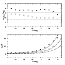
Figure 6: Fractional flux error as a function of magnitude for OGLE bulge catalogs compared to the results from difference image photometry. In the lower panel we show the median scatter in 12 magnitude bins after removing 10% of the high points to allow for variables. The solid points are the data for SC4, a very dense field, and the open circles for SC10, a relatively sparse field. The short dashed line indicates the scatter in difference image photometry (the fit from Figure 3). The long dashed and solid lines are the same as the short dashed line, but multiplied by 1.7 and 3.0 respectively. The upper panel shows the improvement factors: the same data as in the lower panel, divided by the short dashed line. The falling trend in the improvement factors towards the faint stars is artificial, and comes from the fact that the selection criteria for frames used in the OGLE catalog entries are tighter for fainter stars.

Figure 7: Comparison of the difference image photometry with DoPhot output in the OGLE database for three sample microlensing events. Each of the three panels shows two light curves of a very faint, average and bright star, from top to bottom. Despite the fact that our light curves typically contain a few more points (we allowed even the worst seeing frames), image subtraction provides dramatically reduced scatter and improved information about events.

4.1 Noise characteristics

Ideally one would test the properties of the photometry using a sample of constant stars. However our catalogs contain only suspected variables. Some of the bright non-variable stars are included in the catalog because at the time the variables were selected we did not know the exact behavior of the noise, but they are not typical. The next best stars are microlensed stars: these have a long base line, when the light is essentially constant and the form of light variation is known in typical cases. The full catalog of microlensing events from this analysis will be published shortly. Here we will only make the tantalizing statement that 512 events were found in all 49 fields, about a factor of 2 increase compared to the OGLE catalog (Udalski et al. 2000) with the appropriate adjustments for differing selection criteria. Perhaps even more significant is the fact that finally a sample of 305 well covered events with good S/N could be fully algorithmically extracted from the OGLE data without any unwanted ghost light curves coming through the selection process. The MACHO team recorded a similar fractional increase in the number of events detectable using their own algorithm (Alcock et al. 1999b).

Noise properties were derived from the residuals of individual measurements around the best fit microlensing curve. Points inside the region $t_{\rm max}\pm 2t_{0}$ were rejected ($t_{\rm max}$ is the moment of maximum light and $t_{0}$ is the Einstein radius crossing time). Also events with evidence for systematic departures from classic point source microlensing curve and evidence of source variability were excluded from the analysis. Each residual was normalized by the photon noise estimate for the corresponding photometric point. Then stars were grouped according to the total flux on the template at their location filtered through the PSF (the one in the catalog entry, Section 3.9). All residuals coming from light curves of stars in a given group were merged into one distribution.

For each group we calculated the half width of the region containing 68.3% of residuals and centered on 0, a robust estimator of the width of the Gaussian distribution. In Figure 3 we plot thus estimated $\sigma$ as a function of flux. A red clump star at $I\simeq 15.5$ mag has the flux around 1300 counts in our units. The width of the log flux bin corresponds to 0.5 mag, as indicated by horizontal error bars. At the faint end we find that the noise (standard deviation) is only 17% above the Poisson limit. The data is well fitted by the following simple law:

$${\sigma_{F}\over\sigma_{\rm ph}}=1.1671~{}\root \of{1+8.736\times 10^{-4}F}.$$ (11)

As we move towards brighter stars this excess increases due to systematic effects related to seeing and PSF uncertainty, first very slowly and then faster. Alard and Lupton (1998) provide a possible explanation in terms of the atmospheric turbulence. In Figure 4 we also show the error estimate given in our databases, as a function of flux. This is basically photon noise multiplied by 1.6 and propagated through the PSF fit. The formula

$${\rm S/N_{db}}=4.8~{}{F\over\root \of{F+800}}$$ (12)

provides a good fit to the data. Therefore the actual S/N ratio is:

$${\rm S/N=1.6~{}{\left(\sigma_{F}\over\sigma_{ph}\right)}^{-1}S/N_{db}}.$$ (13)

The solid curve shown in Figure 3 can be used to rescale the error bars in order to improve the consistency of the light curves. Then we may also consider renormalized residuals with this new rescaled noise and check their integrated distribution, that is all points from stars of all magnitudes. The resulting histogram is shown in Figure 5 along with the Gaussian distribution of the same norm and $\sigma$ estimated from the 68th percentile of the histogram. The departures from gaussianity are very small. The cumulative distributions in the lower panel of Figure 5 reveal a non-Gaussian tail at the level of only $\sim 0.7$%. Regular, understandable behavior of the noise will certainly have a positive impact on the amount and quality of the information derived from these data.

To further evaluate the difference image photometry we compared the results of Figures 3 and 4 to the photometry obtained with DoPhot in the standard OGLE pipeline. To simplify our task, we used stars from the OGLE bulge catalogs. Each OGLE catalog entry contains the information about the mean and the scatter of the so called “good” measurements, selected using the values of seeing and of the error bar returned by DoPhot compared to the typical errors for stars in a field of a given density (Udalski et al. 1993, Szymański & Udalski 1992). We considered stars in 12 magnitude bins between $I$=13 and 19 mag detected in two fields: SC4, a dense field, and SC10, a relatively sparse field. In SC4 and SC10 on the best frame DoPhot detects about 770,000 and 460,000 stars respectively. In each magnitude bin we reject 10% of the stars with the largest scatter, a conservative allowance for real variability. In the remaining group of stars we adopt median scatter as the measure of typical behavior. The results are summarized in Figure 6. The points indicate the actual median scatter from OGLE database. We also show three lines which correspond to the scatter in image subtraction method (short dashed) and its two copies rescaled by factors 1.7 (long dashed) and 3.0 (solid). In the entire range of fluxes difference image photometry is at least 2 times more accurate, sometimes almost 4 times. The fact that the improvement seems to decline for faint stars is an artifact of the cleaning procedure used by OGLE. Figure 7 is a nice illustration of what can be accomplished. For each of the three sample microlensing events with sources of differing brightness we show two light curves. One obtained with image subtraction software and one with DoPhot. The improvement is striking. In the case of star SC3 792295 the binary nature of the event is obvious in the Difference Image Analysis, while with DoPhot photometry alone one would have to accept a large uncertainty margin for such hypothesis.

4.2 Accuracy of the centroid

Figure 8: Quality of the centroid as a function of S/N ratio in the intensity peak used for the estimate. The solid points represent the scatter measured in 100 simulated realizations of a 3$\times$3 neighborhood of the intensity peak. The open points correspond to the actual scatter for bright isolated stars measured in 100 frames. At the bright end the atmosphere limits the accuracy to about 0.06–0.10 pixels (0.024–0.040 arcsec), a much larger value than suggested by the simulation. Near S/N=15 and below centroid suddenly becomes uncertain.

To complete the discussion of how the codes perform we summarize the properties of the centroid. The expectation is that the random error in position of the intensity peak depends on the width of the peak (curvature), the signal to noise ratio and the exact centroid position with respect to the center of the pixel. This is independent of whether the peak is a normal image of a star or was obtained by coadding peaks from variables on difference frames, as in the procedure of centroid finding for variables in our catalog (Section 3.9). In Figure 8 we compare two estimates. The first estimate comes from a simulation (solid points). We generated fake 3$\times$3 pixel peak neighborhoods of our microlensing events using their actual catalog centroids. The photon noise was included in the simulation and normalized to the total S/N ratio in the peak from which the catalog centroid was calculated. Figure 8 shows the standard deviation of 100 realizations of the experiment using our standard centroiding procedure of Section 3.9. The range of seeing is relatively narrow in entire data set so the correlation with S/N clearly shows. For S/N$>$20 the position is accurate to a small fraction of a pixel, but below S/N $\sim 15$ the uncertainty explodes and we can only assume that the star is where the brightest pixel is. Open points in Figure 8 are real measurements. They correspond to standard deviations of 100 independent centroid estimates for 56 bright stars detected on 100 frames resampled to the same pixel grid (before subtraction). The atmospheric limit for the accuracy of the centroid is about 0.06 pixels in our data (Alard & Lupton 1998). The anomalous refraction, which depends on the color of the star, should be small in the spectral region as red as the $I$-band, but it can only further increase this limit. Obviously, very low error bars on the positions in the simulation are unrealistic. We note full consistency of the results for bright stars with the scatter around the fit to the coordinate transformation. Our conclusion from Figure 8, for variables and stars in normal frames alike, is that for S/N$>$20 in the peak used for centroiding the accuracy is limited by the atmosphere to 0.06–0.10 pixels (0.024–0.040 arcsec), while below S/N $\sim 15$ suddenly becomes large. For the variables in our database, the difference light curve and the seeing data can be used to recover the above S/N ratio, which in turn gives a rough estimate of the centroid error.

5 Calibration of fluxes

Figure 9: Transformation between raw DoPhot magnitudes and our flux units for SC1 field. The best fit proportionality factor from 120 bright, isolated stars is 7.601, with about 1% uncertainty. The lower panel shows the ratio of the data to the best fit.

The basic type of information delivered by image subtraction is slightly different than that from conventional photometry. Difference imaging returns relative photometry in linear flux units, that is the light curve from which some constant flux has been subtracted. This value depends on the brightness of the object in question on frames used to construct the reference image. There is no way to tell what the percentage amplitude of the variation is, unless we obtain additional information with other means. To put the light curve on a magnitude scale, one needs the source flux on the reference image, the one which has been subtracted from all frames. Equation 14 helps to clarify this concept:

$$m_{i}=C-2.5\log(f_{0}+\Delta f_{i}).$$ (14)

Difference imaging measures $\Delta f_{i}$, however certain applications require $f_{0}$, and that must be measured separately, usually with the use of the PSF photometry on the reference image. This has been known in the past as AC signal vs. DC signal. Conventional PSF photometry measures $(f_{0}+\Delta f_{i})$ for each frame separately, however in crowded fields the noise is pushed far above the photon statistics, and the error distribution is no longer Gaussian due to complicated systematics of the multi-PSF fits in the presence of seeing variations. In image subtraction, on the other hand, we can make very accurate measurements of $\Delta f_{i}$, and $f_{0}$ will be no less accurate than in the previous case — we can always run DoPhot on the reference image.

A separate issue is the zero point calibration, by which we mean the correspondence between the computed number of counts and the flux or magnitude in a standard photometric system. In the simplest case there will be a constant proportionality factor between the instrumental and standard fluxes. Image subtraction brings one little complication here. There may be a different transformation of flux units for $\Delta f_{i}$ and $f_{0}$ due to different normalizations of the PSF in the software or more subtle effects like differing aperture corrections. Therefore in Equation 14 before we can set the $C$ constant, we need to ensure that $\Delta f_{i}$ and $f_{0}$ are measured consistently.

The conversion factor between our difference fluxes and the absolute DoPhot fluxes was determined using isolated candidate variables from our catalogs, for which we could identify a “DoPhot” star within 0.1 pixels. For each variable we estimated the contaminating flux of the neighboring stars on the reference image using coordinates of all detectable stars within 10 pixels and a Gaussian PSF model with the approximate FWHM value. We only used variables contaminated by less than 0.5% according to the above estimate. For such variables the simple photometry from our DIA catalog entry is not influenced by crowding and should be very accurate. Only a small fraction of all stars, and even fewer candidate variables, can satisfy this strict limit, nevertheless there are enough for a good fit to a straight line. Figure 9 shows the data for SC1 field and a one parameter fit to all 120 points. The best fit value of the proportionality factor is 7.601 with 1% uncertainty. Individual fits for all fields give about the same scatter in the resulting slope.

The approximate zero point shift for OGLE data between raw DoPhot magnitudes and standard $I$ band magnitudes can be useful for comparisons. The offset of 25.6 mag added to the DoPhot output provides a crude match.

6 Practical considerations

6.1 Computing power requirements

The computer resources required for difference image photometry are not that different from those needed for DoPhot working in fixed position mode. However, there is plenty of room for inefficiencies if large amounts of data are approached incorrectly. A set of 324 2k$\times$8k images (11 GB of pixel data) takes about 5 days to process with the code compiled and -O3 optimized using GNU gcc compiler on Pentium III 500 MHz PC with 384 MB of RAM memory. I do not recommend running our pipeline on comparably sized data sets with less computing power. About 80% of the computing time is approximately equally shared between two procedures: the expansion of the least-squares matrix for constant kernel to the spatially variable case, and the LU decomposition. Profile experiments with gprof showed that the code is not limited by the disk or memory access. Images taken in still frame mode would eliminate most of the PSF variability present in the current data, and would allow much larger subframes than ours to be processed with the same order of polynomial fits. Because the computing time rapidly increases for higher order spatial dependence of the kernel, more throughput could be achieved. In the case of the main subtracting program it is also very inefficient to process frames one by one. The main calculation, that of the least-squares matrix, can be done once for the entire series of images. Our pipeline can be adapted to online systems; the reference image and the least-squares matrix would be prepared at the beginning of the real time processing and stored. At a later time this would allow processing a single frame as quickly as in the current setup and facilitate nearly real time photometry.

6.2 Availability of the data

As an attachment to the present paper we offer the access to difference photometry for SC1 field, the first of the OGLE-II bulge fields. The data and the programs can be found at http://astro.princeton.edu/$\sim$wozniak/dia . README file explains the details. The distribution includes a catalog of 4597 candidate variables, the database of photometric measurements for all variables in the catalog, a reference image (256 sections), DoPhot photometry on the reference image, and the magnitude zero points for each of the 256 sections. For easy access the images are FITS files (85 MB) and the photometric measurements are gzip compressed ASCII tables (25 MB). All coefficients derived in this paper will apply for SC1 data and future releases. We believe that our pipeline can still be significantly improved, suggestions are welcome and should be sent to the author by email. Extracting variability from difference images without allowing too many spurious objects is a problem of particular interest. Therefore we include with the above data a series of difference frames for 1k$\times$1k region of the full field (1 GB), which should be a good test sample for alternative tools.

7 Summary

I have presented a photometric pipeline based on the Alard & Lupton optimal image subtraction algorithm and capable of processing very large data sets in automated fashion, as is necessary in microlensing searches. The performance was evaluated based on complete reanalysis of 3 observing seasons of data for 49 Galactic bulge fields, amounting to 11,000 images or 380 GB. The photometry obtained in the course of this project will be gradually published. Currently the data for one of the bulge fields is available from anonymous ftp, and we plan to release the data for the remaining fields. Perhaps for the first time, a very weakly filtered large sample of suspected variable stars is publicly available for detailed studies. The overall noise properties are exceptionally good for this kind of massive variability search in crowded fields. The error distribution is nearly Gaussian with $\sim 0.7$% of the points in the non-Gaussian wings. The scatter in the photometry for the faint stars is close to 1.17 times photon noise. For brighter stars this ratio rises due to systematics, nevertheless compared with DoPhot, our photometry is at least 2–3 times better over the entire range of the observed magnitudes. At the bright end, $I\/\sim$11–13 mag, the random errors are about 0.005 mag. Sensitivity to microlensing and the amount of information that can be inferred from statistical analyses improve accordingly. The most striking example is a factor of 2 increase in the number of detected microlensing events. The modular structure of the pipeline provides a sound basis for future development of the implementation.

References

- (1) Alard, C., 2000, A&AS, 144, 363
- (2) Alard, C., & Lupton, R. H., 1998, ApJ, 503, 325
- (3) Alcock, C., et al., 1999a, ApJ, 521, 602
- (4) Alcock, C., et al., 1999b, ApJS, 124, 171
- (5) Crotts, A., 1992, ApJ, 399, L43
- (6) Han, C., 1997, ApJ, 484, 555
- (7) Hogg, D. W., 2000, AJ, submitted (astro-ph/0004054)
- (8) Nemiroff, R. J., 1994, AJ, 435, 682
- (9) Olech, A., Woźniak, P. R., Alard, C., Kaluzny, J., & Thompson, I. B., 1999, MNRAS, 310, 759
- (10) Paczyński, B., 1996, ARAA, 34, 419
- (11) Phillips, A. C., & Davis, L. E., 1995, ASP conf. series, 77, Astronomical Data Analysis Software and Systems IV, ed. R. A. Shaw et al., 297
- (12) Press, W. H., Teukolsky, S. A., Vetterling, W. T., & Flannery, B. P., 1992, Numerical Recipes in C. The Art of Scientific Computing., (2d ed.; New York: Cambridge University Press)
- (13) Reiss, D. J., Germany, L. M., Schmidt, B. P., & Stubbs, C. W., 1998, AJ, 115, 26
- (14) Szymański, M., & Udalski, A., 1992, Acta Astron., 43, 91
- (15) Tomaney, A. B., & Crotts, A. P., 1996, AJ, 112, 2872
- (16) Udalski, A., Szymański, M., Kałużny, J., Kubiak, M., & Mateo, M., 1993, Acta Astron., 43, 69
- (17) Udalski, A., Kubiak, M., & Szymański, M., 1997, Acta Astron., 47, 319
- (18) Udalski, A., Żebruń, K., Szymański, M., Kubiak, M., Pietrzyński, G., Soszyński, I., & Woźniak, P., 2000, Acta Atron., 50, 1
- (19) Schechter, P. L., Mateo, M. L., & Saha, A., 1995, PASP, 105, 1342
- (20) Woźniak, P. R., Alard, C., Udalski, A., Szymański, M., Kubiak, M., Pietrzyński, G., & Żebruń, K., 2000, ApJ, 529, 88
- (21) Woźniak, P. R., & Paczyński, B., 1997, ApJ, 487, 55