Optical Gravitational Lensing Experiment.
OGLE-2000-BUL-43: A Spectacular Ongoing Parallax Microlensing Event.
Difference Image Analysis.

Abstract

We present the photometry and theoretical models for a Galactic bulge microlensing event OGLE-2000-BUL-43. The event is very bright with $I=13.54$ mag, and has a very long time scale, $t_{\rm E}=156$ days. The long time scale and its light curve deviation from the standard shape strongly suggest that it may be affected by the parallax effect. We show that OGLE-2000-BUL-43 is the first discovered microlensing event, in which the parallax distortion is observed over a period of 2 years. Difference Image Analysis (DIA) using the PSF matching algorithm of Alard & Lupton enabled photometry accurate to 0.5%. All photometry obtained with DIA is available electronically. Our analysis indicates that the viewing condition from a location near Jupiter will be optimal and can lead to magnifications $\sim 50$ around January 31, 2001. These features offer a great promise for resolving the source (a K giant) and breaking the degeneracy between the lens parameters including the mass of the lens, if the event is observed with the imaging camera on the Cassini space probe.

1. Introduction

Gravitational microlensing was originally proposed as a method of detecting compact dark matter objects in the Galactic halo (Paczyński 1986). However, it also turned out to be an extremely useful method to study Galactic structure, mass functions of stars and potentially extra-solar planetary systems (for a review, see Paczyński 1996). Most microlensing events are well described by the standard light curve (e.g., Paczyński 1986). Unfortunately, from these light curves, one can derive only a single physical constraint, namely the Einstein radius crossing time, which involves the lens mass, various distance measures and relative velocity (see §4). This degeneracy means that the lens properties cannot be uniquely inferred. Therefore any further information on the lens configuration is of great importance. Microlensing events that exhibit parallax effects provide this type of information. Such effects can occur when the event is observed simultaneously from two different positions in the Solar system (Refsdal 1966) or when the event lasts long enough that the Earth’s motion can no longer be approximated as rectilinear during the event (Gould 1992). Both of these effects will be directly relevant to the current paper. The first parallax microlensing event was reported by the MACHO collaboration toward the Galactic bulge (Alcock et al. 1995), and the second case (toward Carina) was discovered by the OGLE collaboration and reported in Mao (1999). Additional parallax microlensing candidates have been presented in a conference proceeding (Bennett et al. 1997). In this paper, we report a new parallax microlensing event, OGLE-2000-BUL-43. This bulge event was discovered well ahead of the peak by the Early Warning System (Udalski et al. 1994), and attracted attention due to its extreme brightness and very long time scale.

The unusually long duration of the event ($t_{\rm E}\sim 156\,$days) combined with the extremely small velocity of the magnification pattern on the plane of the observer ($\tilde{v}\sim 40\,{\rm\,km\,s^{-1}}$, i.e., hardly faster than the motion of the Earth), imply that the parallax effect is not only detectable, but measurable very precisely. To make the most of this possibility, we employ difference image analysis (DIA, Woźniak 2000) to optimize the photometry (§2).

The parallax measurement that we present here yields not only the size of the Einstein radius projected onto the observer plane ($\tilde{r}_{\rm E}\approx 3.62\,$AU) but also the direction of lens-source relative motion in the heliocentric coordinate system. By combining these two, we can predict the light curve seen by any observer in the solar system as a function of time. In particular, we predict that as seen from the Cassini spacecraft around January 31, 2001, the lens and source will have an extraordinarily close separation and hence the source will be highly magnified. Unless the lens turns out to be very massive ($M\gtrsim 0.8\,M_{\odot}$) and close ($D_{\rm d}\lesssim 1\,$kpc), such a separation would permit resolution of the source and hence measurement of the the angular Einstein radius, $\theta_{\rm E}$ (Alcock et al. 1997, 2000; Albrow et al. 1999, 2000, 2001; Afonso et al. 2000). Gould (1992) showed that by combining measurements of $\tilde{r}_{\rm E}$, $\theta_{\rm E}$ and the Einstein radius crossing time ($t_{\rm E}$), one could obtain a complete solution of the event,

$$M = {c^{2}\over 4G}\tilde{r}_{\rm E}\theta_{\rm E},$$ (1)

$$D_{\rm rel} = {\tilde{r}_{\rm E}\over\theta_{\rm E}}\equiv{{\rm AU}\over\pi_{\rm rel}},$$ (2)

$$\mu_{\rm rel} = {\theta_{\rm E}\over t_{\rm E}},$$ (3)

where $D_{\rm rel}=D_{\rm d}D_{\rm s}/(D_{\rm s}-D_{\rm d})$, $\pi_{\rm rel}={\rm AU}/D_{\rm d}-{\rm AU}/D_{\rm s}$ is the lens-source relative parallax, $\mu_{\rm rel}$ is the lens-source relative proper motion, and $D_{\rm d}$ and $D_{\rm s}$ are the distances to the lens and source, respectively. See also Gould (2000). Since the source is quite bright even at baseline $(I=13.54,V=15.65)$ it should be easily measurable by the Cassini probe. Cassini photometry would therefore very likely yield the first mass measurement of a microlensing event.

The outline of the paper is as follows. In §2 we describe observations, in §3 we describe our photometric reduction method, §4 contains the details of model fitting and predicted viewing conditions, in §5 we describe potential scientific returns of Cassini observations and finally in §6, we briefly summarize and discuss our results.

2. Observations

All observations presented in this paper were carried out during the second phase of the OGLE experiment with the 1.3-m Warsaw telescope at the Las Campanas Observatory, Chile, which is operated by the Carnegie Institution of Washington. The telescope was equipped with the “first generation” camera with a SITe ${2048\times 2048}$ CCD detector working in the drift-scan mode. The pixel size was 24 $\mu$m giving the scale of 0.417$\arcsec$ per pixel. Observations of the Galactic bulge fields were performed in the “medium” reading mode of the CCD detector with the gain 7.1 e^-/ADU and readout noise about 6.3 e^-. Details of the instrumentation setup can be found in Udalski, Kubiak & Szymański (1997).

The OGLE-2000-BUL-43 event was detected by the OGLE Early Warning System (Udalski et al. 1994) in mid-2000. Equatorial coordinates of the event for 2000.0 epoch are: $\alpha_{2000}=18^{\rm h}08^{\rm m}43\makebox[0.0pt][l]{.}^{\rm s}04$, $\delta_{2000}=-32^{\circ}24{{}^{\prime}}39\makebox[0.0pt][l]{.}{{}^{\prime\prime}}5$, ecliptic coordinates are: $\lambda=271\makebox[0.0pt][l]{.}^{\circ}863$, $\beta=-8\makebox[0.0pt][l]{.}^{\circ}986$ and Galactic coordinates are $l=359\makebox[0.0pt][l]{.}^{\circ}467$, $b=-6\makebox[0.0pt][l]{.}^{\circ}036$. Figure 1 is a finding chart showing the $120\arcsec\times 120\arcsec$ region centered on the event. Observations of this field started in March 1997, and continued until November 22, 2000. The bulge observing season usually ends at the beginning of November, therefore the latest observations of OGLE-2000-BUL-43 were made in difficult conditions with the object setting shortly after the sunset, when the sky is still quite bright. Fortunately the source was bright enough so that poor seeing and high backgrounds were not a significant problem in the DIA analysis.

The majority of the OGLE-II frames are taken in the $I$-band. For the BUL_SC7 field 330 $I$-band and 9 $V$-band observations were collected. Udalski et al. (2000) gives full details of the standard OGLE observing techniques and the DoPhot photometry is available from OGLE web site at http://www.astrouw.edu.pl/$\sim$ogle/ogle2/ews/ews.html.

3. Photometry

Our analysis includes all $I$-band observations of the BUL_SC7 field. We used the DIA technique to obtain the light curves of the OGLE-2000-BUL-43 event. Our method is based on the recently developed optimal PSF matching algorithm (Alard & Lupton 1998; Alard 2000). Unlike other methods that use divisions in Fourier space (Crotts 1992, Phillips & Davis 1995, Tomaney & Crotts 1996, Reiss et al. 1998, Alcock et al. 1999), the Alard & Lupton method operates directly in real space. Additionally it is not required to know the PSF of each image to determine the convolution kernel. Woźniak (2000) tested the method on large samples and showed that the error distribution is Gaussian to better than 1%. Compared to the standard DoPhot photometry (Schechter, Mateo, & Saha 1993), the scatter was always improved by a factor of 2–3 and frames taken in even the worst seeing conditions gave good photometric points.

Our DIA software handles PSF variations in drift-scan images by polynomial fits. Even then it is required that the frames are subdivided into 512$\times$128 pixel strips because PSF variability along the direction of the scan is much faster than across the frame. The object of interest turned out to be not too far from the center of one of the subframes selected automatically, therefore we basically adopted the standard pipeline output for that piece of the sky without the need to run the software on the full format. Minor modifications included more careful preparation of the reference image and calibration of the counts in terms of standard magnitude system.

First, from the full data set for the BUL_SC7 field we selected 20 frames with the best seeing, small shifts relative to OGLE template and low background level. More weight was assigned to the PSF shape and quality of telescope tracking in the analyzed region during the selection process. These frames were co-added to create a reference frame for all subsequent subtractions. Preparation of the reference image was absolutely critical for the quality of the final results.

Next we ran the DIA pipeline for all of our data to retrieve the AC signal (variable part of the flux) of our lensed star. The software rejected only 9 frames due to very bad observing conditions or very large shifts in respect to the reference image. Our final light curve contains 321 observations. To calibrate the result on the magnitude scale we ran DoPhot on the reference image. The magnitude zero point ($I=13.54,V=15.65$) was obtained by comparing our DoPhot photometry with the OGLE database.

The DIA light curve is shown in Figure 2. The scatter in the photometry is 0.5% and is dominated by systematics due to atmospheric turbulence and PSF variations. The individual error bars returned by the automated massive photometry pipeline (Woźniak 2000) proved to be over-estimated when compared to the scatter around the best fit model (§4). Most likely this is a combined result of individual care during data processing for OGLE-2000-BUL-43 and relatively low density of stars in the BUL_SC7 field. The errors were re-calibrated so as to enforce $\chi^{2}$ per degree of freedom to be unity in the best-fit model with parallax (see §4 and Table 1).

We would like to stress the fact that it is the accuracy achieved here with the DIA method which enabled a detailed study of the lens parameters. Figure 3 presents the distribution of residuals with respect to the model (see §4) for measurements with the DIA pipeline. Maximal differences between the classical single point microlensing model and the parallax fit are indicated by dashed vertical lines. One notices that the scatter of the photometry is small enough to analyse the parallax effect. Additionally our data set contains 82 more points than the OGLE EWS light curve. The difference is because the lowest grade frames are rejected in the standard DoPhot analysis. The DIA photometry data file is available from the OGLE anonymous FTP server: ftp://sirius.astrouw.edu.pl/ogle/ogle2/BUL-43/bul43.dat.gz.

In Figure 4 we present the Color-Magnitude Diagram for the BUL_SC7 field. The position of the lensed star (marked by a cross) suggests that the source is a K giant. For later studies of the finite source size effect (§5), we would like to estimate the angular diameter of the star. In order to do this, we first need to estimate the dereddened color and magnitude of the star. For this purpose, we use the red-clump giants that have well calibrated dereddened colors and magnitudes. We adopt the average color and magnitude of red-clump giants in Baade’s window from the previous studies (Paczyński et al. 1999),

$$(V-I)_{\rm RC,0}=1.11,~{}~{}I_{\rm RC,0}=14.37.$$ (4)

From Figure 4, the red-clump stars in the BUL_SC7 field have

$$(V-I)_{\rm RC}=1.67\pm 0.02,~{}~{}I_{\rm RC}=15.15\pm 0.05.$$ (5)

Hence we have

$$E(V-I)=(V-I)_{\rm RC}-(V-I)_{\rm RC,0}=0.57,$$ (6)

and

$$A_{I}=I_{\rm RC}-I_{\rm RC,0}=0.78.$$ (7)

Taking into account a blending parameter $f=0.91$ (see §4, Table 1) in the $I$-band, we obtain the magnitudes of the lensed star as $I=13.64,V=15.75$. Hence, the intrinsic color and $I$-band magnitude for OGLE-2000-BUL-43 are

$$(V-I)_{0}=(V-I)-E(V-I)=1.54,~{}~{}I_{0}=I-A_{I}=12.86.$$ (8)

Note that these values we derived are somewhat different from those of Schlegel, Finkbeiner & Davis (1998): $A_{I}=0.92$ and $E_{V-I}=0.61$. Our smaller extinction value is consistent with Stanek (1998) who argued that the Schlegel et al. (1998) map over-estimates the extinction for $|b|<5^{\circ}$. Our estimate based on the red-clump giants is also somewhat uncertain because of the metallicity gradient that may exist between Baade’s window ($b=-4^{\circ}$) and the BUL_SC7 field ($b=-6^{\circ}$). Fortunately, this uncertainty in reddening only affects the angular diameter estimate very slightly because the surface brightness-color relation has a slope similar to the slope of the reddening line (see below).

Using the dereddened color and magnitude, we can estimate the angular stellar radius ($\theta_{\star}$) using the empirically determined relation between color and surface brightness (van Belle 1999), independent of the source distance. Transforming van Belle’s relation given in $V$ vs. $V-K$ into $I$ vs. $V-I$ using the color-color relations of Bessel & Brett (1988), one obtains

$$\theta_{\star}=18.9\mu{\rm as}\,\times 10^{(12.90-I_{0})/5}\times[(V-I)_{0}-0.6]$$ (9)

For our star, this gives $\theta_{\star}=18.1\mu{\rm as}$. Using the values from Schlegel et al. (1998), the $\theta_{\star}$ value increases by about 2%. Therefore the estimate of the angular stellar radius is quite robust.

4. Model

We first fit the light curve with the standard single microlens model which is sufficient to describe most microlensing events. In this model, the (point) source, the lens and the observer all move with constant spatial velocities. The standard form is given by (e.g., Paczyński 1986):

$$A(t)={u^{2}+2\over u\sqrt{u^{2}+4}},~{}~{}u(t)\equiv\sqrt{u_{0}^{2}+\tau(t)^{2}},$$ (10)

where $u_{0}$ is the impact parameter (in units of the Einstein radius) and

$$\tau(t)={t-t_{0}\over t_{\rm E}},~{}~{}t_{\rm E}={\theta_{\rm E}\over\mu_{\rm rel}},$$ (11)

with $t_{0}$ being the time of the closest approach (maximum magnification), $\theta_{\rm E}$ the angular Einstein radius, and $t_{\rm E}$ the Einstein radius crossing time. The explicit forms of the angular Einstein radius ($\theta_{\rm E}$) and the projected Einstein radius ($\tilde{r}_{\rm E}$) are

$$\theta_{\rm E}=\sqrt{{4GM\over c^{2}D_{\rm rel}}},~{}~{}\tilde{r}_{\rm E}=\sqrt{{4GMD_{\rm rel}\over c^{2}}}$$ (12)

where $M$ is again the lens mass and $D_{\rm rel}$ is defined below equation (3). For microlensing in the local group, $\theta_{\rm E}$ is $\sim$ mas and $\tilde{r}_{\rm E}$ $\sim$ few AU. Equations (10-12) show the well-known lens degeneracy, i.e., from a measured $t_{\rm E}$, one can not infer the lens mass, distances and kinematics uniquely even if the source distance is known.

To fit the $I$-band data with the standard model, we need a minimum of four parameters, namely, $u_{0},t_{0},t_{\rm E},I_{\rm s}$, where $I_{\rm s}$ is the unlensed $I$-band magnitude of the source. The best-fit parameters (and their errors) are found by minimizing the usual $\chi^{2}$ using the MINUIT program in the CERN library and are tabulated in Table 1 (model S). The resulting $\chi^{2}$ is 9025.2 for 317 degrees of freedom. The large $\chi^{2}$ indicates that the fit is unacceptable. This can also be clearly seen in Figure 2, where we have plotted the predicted light curve as the dotted line. The deviation is apparent in the 2000 observing season. In fact, upon closer examination, the model over-predicts the magnification in the 1999 season as well (see the bottom inset in Figure 2). Since the Galactic bulge fields are very crowded, there could be some blended light from a nearby unlensed source within the seeing disk of the lensed source, or there could be some light from the lens itself. So in the model we can introduce a blending parameter, $f$, which we define as the fraction of light contributed by the lensed source in the baseline ($f=1$ if there is no blending). Note that blending is introduced in our adoption of the magnitude zero point obtained by the DoPhot photometry; the DIA method itself automatically subtracts out the blended light. The inclusion of the blending parameter reduces the $\chi^{2}$ to 2778.4 for 316 degrees of freedom. This model requires a blending fraction $f=0.22$, which is implausible considering the extreme brightness of the lensed star. In any case, the $\chi^{2}$ is better but still far from acceptable. We show below that all these discrepancies can be removed by incorporating the parallax effect.

To account for the parallax effect, we need to describe the Earth motion around the Sun. We adopt a heliocentric coordinate system with the $z$-axis toward the Ecliptic north and the $x$-axis from the Sun toward the Earth at the Vernal Equinox. The position of the Earth, to the first order of the orbital eccentricity ($\epsilon\approx 0.017$), is then (e.g., Dominik 1998 and references therein)

$$x_{\oplus}(t) = A(t)\cos[\xi(t)-\phi_{\gamma}],$$

$$y_{\oplus}(t) = A(t)\sin[\xi(t)-\phi_{\gamma}],$$ (13)

$$z_{\oplus}(t) = 0,$$

where

$$A(t)={\rm AU}\,(1-\epsilon\cos\Phi),~{}~{}~{}\xi(t)=\Phi+2\epsilon\sin\Phi$$ (14)

with $\Phi=2\pi(t-t_{\rm p})/T$, $T=1\,{\rm yr}$, and $\phi_{\gamma}\approx 75\makebox[0.0pt][l]{.}^{\circ}98$ is the longitude difference between the Perihelion ($t_{\rm p}=1546.708$) and the Vernal Equinox ($t\equiv{\rm JD}-2450000=1623.816$) for J2000. The line of sight in the heliocentric coordinate system is as usual described by two angular polar coordinates $(\phi,\chi)$. These two angles are related to the geocentric ecliptic coordinates $(\lambda,\beta)$ by $\chi=\beta$, and $\phi=\pi+\lambda$. Again, for OGLE-2000-BUL-43, $\beta=-8\makebox[0.0pt][l]{.}^{\circ}986$, and $\lambda=271\makebox[0.0pt][l]{.}^{\circ}863$ (see, e.g., Lang 1981 for conversions between different coordinate systems).

To describe the lens parallax effect, we find it more intuitive to use the natural formalism as advocated by Gould (2000), i.e., we project the usual lensing quantities into the observer (and ecliptic) plane. The line of sight vector is given by $\hat{n}=(\cos\chi\cos\phi,\cos\chi\sin\phi,\sin\chi)$ in the heliocentric coordinate system. For a vector, $\vec{r}$, the component perpendicular to the line of sight is given by $\vec{r}_{\perp}=\vec{r}-(\vec{r}\cdot\hat{n})\hat{n}$. For example, the perpendicular component of the Earth position is $\vec{r}_{\oplus,\perp}={\vec{r}_{\oplus}-(\vec{r}_{\oplus}\cdot\hat{n})\hat{n}}$. Thus, a circle in the lens plane ($\vec{r}_{\perp}^{2}=R^{2}$) is mapped into an ellipse in the ecliptic plane, which is given by,

$$r={R\over\sqrt{1-\cos^{2}\chi\cos^{2}(\Theta-\phi)}},$$ (15)

where $\Theta$ is the polar angle in the ecliptic plane. The minor axis and major axis for the ellipse are $R$ and $R/\sin\chi$, respectively.

The lens trajectory is described by two parameters, the dimensionless impact parameter, $u_{0}$, and the angle, $\psi$, between the heliocentric ecliptic $x$-axis and the normal to the trajectory. Note that $u_{0}$ is now more appropriately the (dimensionless) minimum distance between the Sun-source line and the lens trajectory. For convenience, we define the Sun to be on the left-hand side of the lens trajectory for $u_{0}>0$. The lens position (in physical units) projected into the ecliptic plane, $\vec{r}_{\rm L}=(x_{\rm L},y_{\rm L},0)$, as a function of time, is given by

$$x_{\rm L} = u_{0}\tilde{r}_{\rm E}\cos\psi-\tau r_{\rm E,p}(\psi)\sin\psi,$$

$$y_{\rm L} = u_{0}\tilde{r}_{\rm E}\sin\psi+\tau r_{\rm E,p}(\psi)\cos\psi,$$ (16)

$$z_{\rm L} = 0,$$

where $\tau$ and $\tilde{r}_{\rm E}$ are defined in equations (11) and (12), and $r_{\rm E,p}=\tilde{r}_{\rm E}/\sqrt{1-\cos^{2}\chi\sin^{2}(\pi/2+\psi-\phi)}$ is the Einstein radius projected into the ecliptic plane in the direction of the lens trajectory. The expression of $r_{\rm E,p}$ can be derived using equation (15) with $\Theta=\pi/2+\psi$, where the factor $\pi/2$ arises because $\psi$ is defined as the angle between the normal to the trajectory and the $x$-axis. We denote the vector from the lens position (projected into the ecliptic plane) toward the Earth as $\delta{\vec{r}}=\vec{r}_{\oplus}-\vec{r}_{\rm L}$. The component of $\delta{\vec{r}}$ perpendicular to the line of sight is $\delta{\vec{r}}_{\perp}=\delta{\vec{r}}-(\delta{\vec{r}}\cdot\hat{n})\hat{n}$. The magnification can then be calculated using equation (10) with $u^{2}=(\delta{\vec{r}}_{\perp}/\tilde{r}_{\rm E})^{2}$.

In total, seven parameters ($u_{0},t_{0},t_{\rm E},I_{\rm s},\tilde{r}_{\rm E},\psi,f$) are needed to describe the parallax effect with blending. These parameters are again found by minimizing $\chi^{2}$. In table 1, we list the best fit parameters (model P); for this model, the $\chi^{2}$ per degree of freedom is now unity due to our rescaling of errors (see §2). In particular, we find that

$$\tilde{r}_{\rm E}=(3.62\pm 0.16)\thinspace{\rm AU},~{}~{}\psi=(3.024\pm 0.005)\thinspace{\rm rad}.$$ (17)

The correlation coefficient between $\tilde{r}_{\rm E}$ and $\psi$ is $-0.088$. The predicted light curve is shown in Figure 2 as the solid line. The model fits the data points very well. Notice that the model requires a marginal blending with $f=0.911\pm 0.056$. This is expected since the source star is very bright, and it appears unlikely that any additional source can contribute substantially to the total light. We return to the degeneracy of solutions briefly in §6.

Using equations (1-2), and $\tilde{r}_{\rm E}\approx 3.62\,{\rm AU}$, we obtain the lens mass as a function of the relative lens-source parallax

$$M={c^{2}\tilde{r}_{\rm E}^{2}\over 4G}\pi_{\rm rel}=0.23M_{\odot}\left({3.5\,{\rm{kpc}}\over D_{\rm d}}-{7\,{\rm{kpc}}\over D_{\rm s}}\right).$$ (18)

So the lens is likely to be low-mass unless it is unusually close to us ($D_{\rm d}\sim 1\,{\rm{kpc}}$). Combining $\tilde{r}_{\rm E}$ and $t_{\rm E}$, we can also derive the projected velocity of the lens,

$$\tilde{v}=\mu_{\rm rel}D_{\rm rel}={\tilde{r}_{\rm E}\over t_{\rm E}}=(40\pm 2){{\rm\,km\,s^{-1}}}.$$ (19)

The low projected velocity favors a disk-disk lensing event. For such events, the observer, the lens and the source rotate about the Galactic center with roughly the same velocity, and the relative motion is only due to the small, $\sim 10{\rm\,km\,s^{-1}}$, random velocities (see, e.g., Derue et al. 1999). On the other hand, the chance for a bulge source (with its much larger random velocity, $\sim 100{\rm\,km\,s^{-1}}$) to have such a low projected velocity relative to the lens (whether disk or bulge) is small. The low projected speed and the long duration of this event imply that the Earth’s motion induces a large excursion in the Einstein ring, and this large deviation from rectilinear motion makes an accurate parallax measurement possible, even though the event has only barely reached its peak.

The accurate measurement of $\tilde{r}_{\rm E}$ and $\psi$ makes it possible to predict the light curve that would be seen by a hypothetical observer anywhere in the solar system. Figure 5 shows the illumination pattern on January 1.000, 2001 UT. The two elliptical curves are iso-magnification contours for $A=1.342$ and 4, respectively; the outer contour with $A=1.342$ corresponds to the Einstein ‘ring’ in the ecliptic plane. It appears as an ellipse in Figures 5 and 7 because the ecliptic plane is not perpendicular to the source direction (cf. eq. 15). Various filled dots indicate the positions of the source, Earth, Jupiter and Saturn on this date. The open dots indicate the positions of the source and the planets every half a year in the future. From this figure, one can see that the inner contour nearly coincides with the position of Jupiter on January 1, 2001, hence an observer close to Jupiter will see a magnification of about 4; the magnification is even higher somewhat later. The Cassini probe is currently approaching Jupiter, for a fly-by acceleration on its way to Saturn, it is therefore an ideal instrument to observe this event from space. In the next section, we will discuss in some detail the potential scientific returns of Cassini observations.

5. Potential Scientific Returns of Cassini Observations

In Figure 6 we show the light curve of OGLE-2000-BUL-43 for an observer near Jupiter, mimicking the fly-by observations from Cassini. The light curve shows a spectacular peak at JD$\approx$ 2451940.5 (January 31, 2001). Figure 7 illustrates the position of Jupiter with respect to the illumination pattern. It clearly shows that the lens and Jupiter will come very close together and hence one will see a very high magnification around that time.

When the physical impact parameter is comparable to the stellar radius, microlensing light curves are substantially modified by the finite source size effect (Gould 1994; Nemiroff & Wickramasinghe 1994; Witt & Mao 1994). More precisely, when

$$u_{0}\lesssim u_{\star}\equiv{\theta_{\star}\over\theta_{\rm E}}={c^{2}\over 4GM}\tilde{r}_{\rm E}\theta_{\star}={0.008\over M/M_{\odot}},$$ (20)

then finite source size effects will be significant and it becomes feasible to measure $\theta_{\rm E}$, hence providing one more constraint on the lens parameters. Our best-fit model has a minimum impact parameter (in the lens plane) $u_{0}=3.6\times 10^{-3}$, and so unless the lens is very close to us and very massive (eq. 18), the finite source size will be resolved. The inset in Fig. 6 illustrates this effect where we have adopted $\theta_{\rm E}=0.47$ mas. The effect is quite dramatic. In comparison, the effect is negligible for an observer on Earth. Note that the peak of the light curve only depends on $u_{\star}=\theta_{\star}/\theta_{\rm E}$. So the peak can be higher if the angular Einstein radius is larger, and vice versa.

To plan space observations, it is important to estimate the errors in the minimum impact parameter ($u_{0}$) and the peak time ($t_{0}$). We have performed Monte Carlo simulations to estimate their uncertainties (e.g., Press et al. 1992). We find that the 95% confidence limits on $u_{0}$ and $t_{0}$ are $10^{-4}<u_{0}<0.011$ and $1938.3<t_{0}<1941.3$, respectively. It is therefore very likely that the magnification at Jupiter will be very high. The peak time is accurate to about 3 days while the finite source size effect lasts for about twenty days (see the inset in Figure 6). To detect this effect, it is crucial to have at least a few observations during the lens transit across the stellar surface (Peng 1995). If the finite source size effect is indeed observed by Cassini, then we can measure $\theta_{\rm E}$, and this will lead to, for the first time, a complete solution of the lens parameters, including the lens mass, the relative lens-source parallax and proper motions (see introduction). We again emphasize that the determination of mass is independent of the source distance if $\theta_{\rm E}$ is measured (cf. eq. 1).

6. Summary and Discussion

OGLE-2000-BUL-43 is the longest microlensing event observed by the OGLE project. It is also the first event, in which the parallax effect is observed over a 2 year period, making the association of the acceleration term with the motion of the Earth unambiguous. Photometric accuracy at the 0.5% level enabled a detailed study of the event parameters partly removing the degeneracy between the mass, velocity and distance. We conclude that the lens is slow moving, and unless it is unusually close to us, the lens mass is expected to be small.

The main aim of this paper is to strongly encourage further efforts to observe OGLE-2000-BUL-43, as this may lead the first complete determination of the lens parameters. We could even consider a confirmation of the predictions from Figure 6 to be an ultimate proof of our understanding of the microlensing geometry. This is particularly important since the lens model may not be unique. For example, we found another model (see Table 1, model P^′) that has $\chi^{2}=320.8$ but with the blending parameter $f=0.77$. This model predicts a much lower peak ($I_{\rm peak}=12.2$) for an observer close to Jupiter. Even late space observations will be useful for distinguishing these two models. For example, the best-fit model predicts $I=12.7$ and $I=13.0$ on April 1 and May 1, 2001 respectively, while the slightly worse model predicts $I=13.0$ and $I=13.2$ on these dates. The difference between these two models can reach 0.02 mag in the next season for ground-based observations and hence may be detectable from the ground as well. However, the alternative model appears physically unlikely since the source star is so bright that one would expect $f$ close to 1, as found in our best fit model. The blending parameter may also be constrained by spectroscopic observations (Mao, Lennon & Reetz 1998). A high-resolution VLT spectrum has already been taken and is currently being analyzed (K. Gorski 2000, private communication). It will shed further light on the stellar parameters (such as surface gravity) and the radial velocity of the lensed source.

Table 1The best standard model (first row) and the best parallax model with blending (second row) for OGLE-2000-BUL-43. The third rows shows a parallax fit with slightly worse $\chi^{2}$ (see §6).

Model	$t_{0}$	$t_{\rm E}$ (day)	$u_{0}$	$I_{\rm s}$	$\psi$	$\tilde{r}_{\rm E}$ (AU)	f	$\chi^{2}$
S	$1898.7\pm 0.1$	$169.6\pm 0.3$	$0.0\pm 0.002$	$13.5366\pm 0.0004$	—	—	—	9025.2
P	$1893.4\pm 1.0$	$156.4\pm 4.4$	$0.27\pm 0.01$	$13.5406\pm 0.0004$	$3.024\pm 0.005$	$3.62\pm 0.18$	$0.911\pm 0.056$	314
P′	$1842.5\pm 0.9$	$158.2\pm 4.2$	$-0.11\pm 0.01$	$13.5406\pm 0.0004$	$3.017\pm 0.007$	$4.79\pm 0.22$	$0.77\pm 0.04$	320.8

Figure 1.— Finding chart for the OGLE-2000-BUL-43 microlensing event. The size of $I$-band subframe is ${120\arcsec\times 120}\arcsec$; North is up and East to the left.

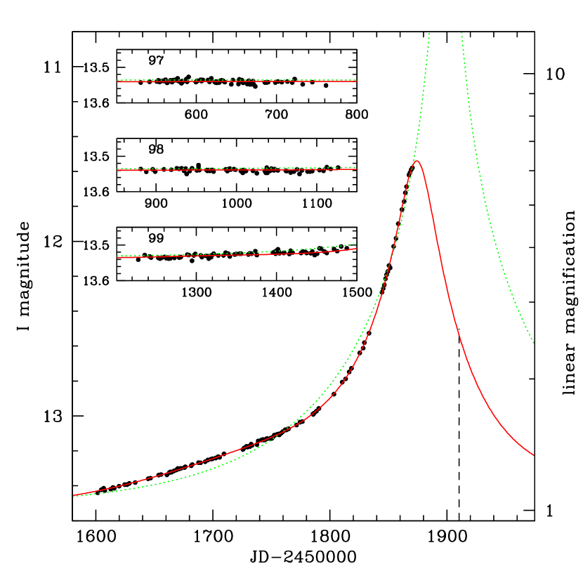
Figure 2.— $I$-band light curve for the microlensing event OGLE-2000-BUL-43. The magnitude scale is shown on the left $y$-axis, while linear magnification is shown on the right $y$-axis. The dotted line is the standard model while the solid line is the best-fit model that takes into account the parallax effect and blending (second row in Table 1). The vertical dashed line marks January 1, 2001, 0UT. The three insets show the the data points for the 1997, 1998 and 1999 seasons, respectively.

Figure 3.— Distribution of residuals with respect to the model for measurements with the DIA pipeline. Width of the bin is 0.005 mag. Sigmas of fitted Gaussian is 0.0055 mag. Additional dashed vertical lines indicate the largest differences between the classical single point microlensing model and the parallax fit.

Figure 4.— Color-magnitude diagram of the BUL_SC7 field. Only about 10% of field stars are plotted by tiny dots. Position of OGLE-2000-BUL-43 event is marked by cross in the circle.

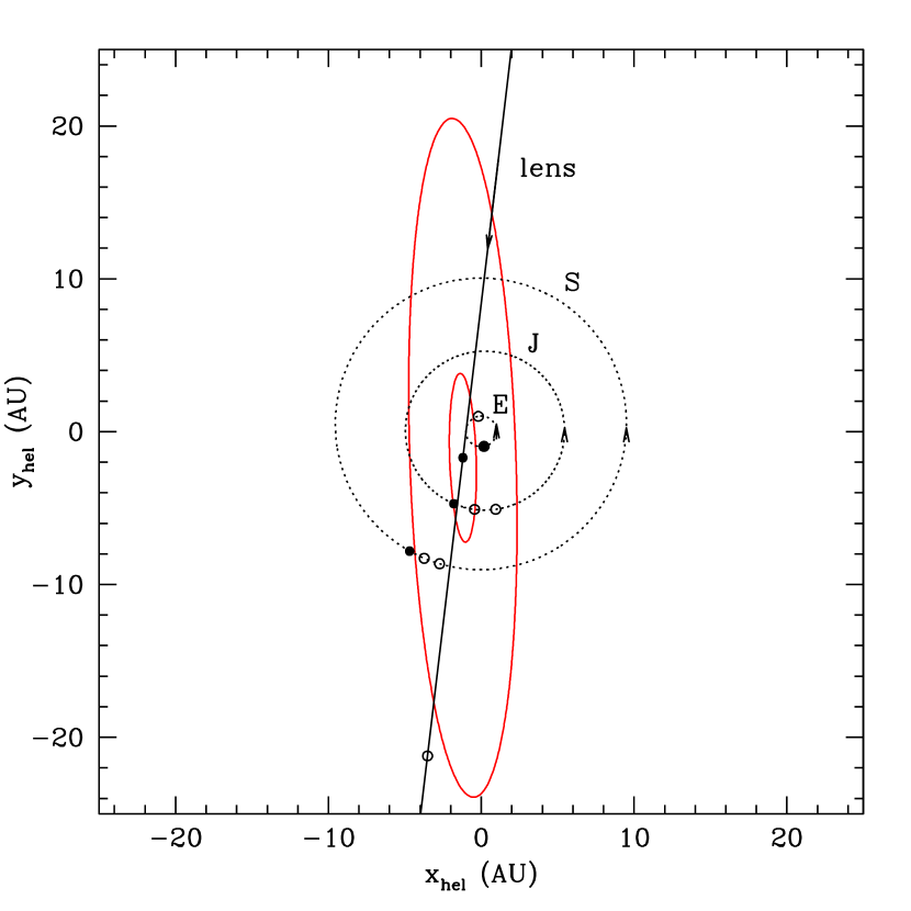
Figure 5.— Illumination patterns for OGLE-2000-BUL-43 in the heliocentric ecliptic coordinates on January 1, 2001, 0UT. The $+x$-axis points from the Sun toward the Earth on the day of Vernal Equinox. The two solid elliptical curves are the iso-magnification contours with magnification 1.342 and 4, respectively. The three dotted circles are the orbits of the Earth, Jupiter and Saturn, respectively. The solid filled dots on the Earth, Jupiter and Saturn orbits indicate their positions on January 1, 2001, while the open dots indicate their positions every half a year in the future. The straight line indicates the lens trajectory and the dot symbols have the same meaning as those on the planetary orbits. The directions of motions are indicated by arrows. Notice that the whole illumination pattern (iso-magnification contours) comoves with the lens.

Figure 6.— Light curve for OGLE-2000-BUL-43 as seen by an observer close to Jupiter. Notice that it reaches a much higher peak around January 31, 2001 than that on the Earth. The vertical dashed line marks January 1, 2001, 0UT (corresponding to the filled dots in Figure 5). The magnitude scale is shown on the left $y$-axis, while linear magnification is shown on the right $y$-axis. The dotted line shows the magnification for a point source while the solid line illustrates the finite source size effect. The inset shows the light curve close to the peak of the light curve.

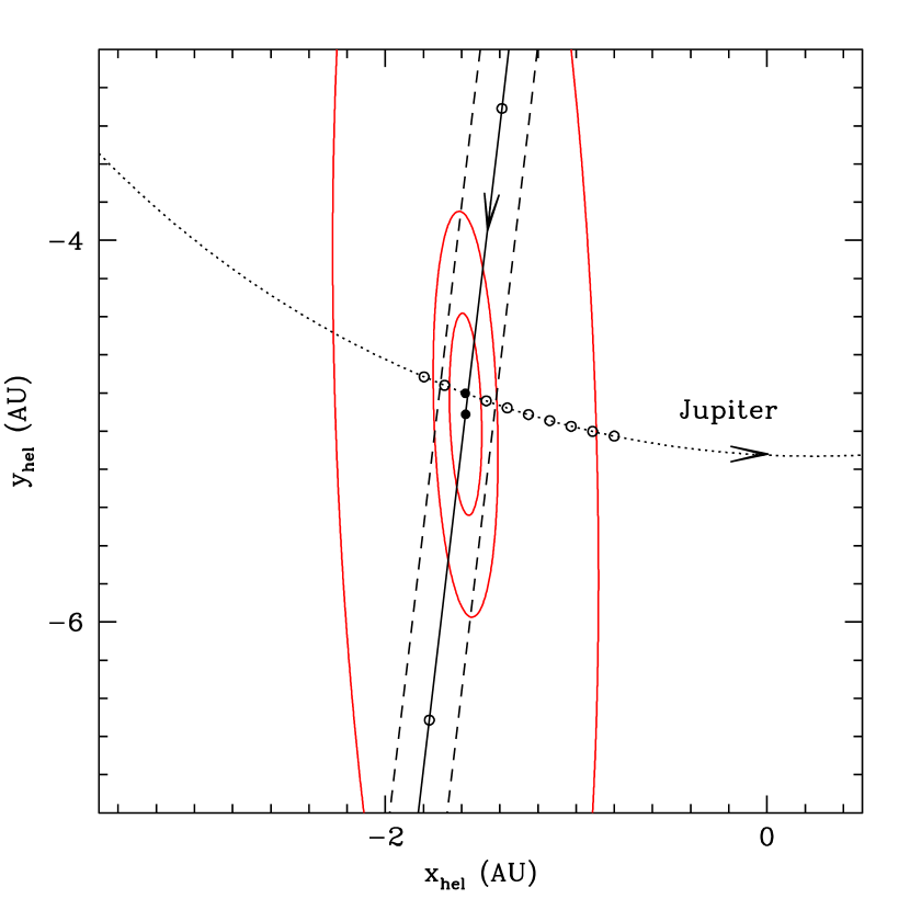
Figure 7.— Illumination patterns for OGLE-2000-BUL-43 in the heliocentric ecliptic coordinates on January 31, 2001, 0UT. The notations are similar to those in Figure 5. The filled dots correspond to $t=1840.5$ while the open dots are separated by 15 days. The contours correspond to magnifications of 5, 20 and 40 (from outer to inner), respectively. The two dashed lines bracket roughly the region that the finite source size effect can be observed.

References

- (1)
- (2) Afonso, C., et al., 2000, ApJ, 532, 340
- (3)
- (4) Alard, C., & Lupton, R. H., 1998, ApJ, 503, 325
- (5)
- (6) Alard, C., 1999, A&A Suppl., 2000, 144, 363
- (7)
- (8) Albrow, M.D., et al., 1999, ApJ, 522, 1022
- (9)
- (10) Albrow, M.D., et al., 2000, ApJ, 534, 894
- (11)
- (12) Albrow, M.D., et al., 2001, ApJ, 549, 000
- (13)
- (14) Alcock, C., et al., 1995, ApJ, 454, L125
- (15)
- (16) Alcock, C., et al., 1997, ApJ, 491, 436
- (17)
- (18) Alcock, C., et al., 1999, ApJ, 521, 602
- (19)
- (20) Alcock, C., et al., 2000, ApJ, 541, 270
- (21)
- (22) Bennett, D. P., et al. 1997, BAAS, 191, 8303
- (23)
- (24) Bessel, M.S., & Brett, J. M. 1988, PASP, 100, 1134
- (25)
- (26) Crotts, A., 1992, ApJ, 399, L43
- (27)
- (28) Derue, F. et al., 1999, A&A, 351, 87
- (29)
- (30) Dominik, M., 1998, A&A, 329, 361
- (31)
- (32) Gould, A., 1992, ApJ, 392, 442
- (33)
- (34) Gould, A. 1994, ApJ, 421, L71
- (35)
- (36) Gould, A., 2000, ApJ, 542, 785
- (37)
- (38) Lang, K.R., 1980, Astrophysical Formulae (Springer-Verlag: Berlin), 504
- (39)
- (40) Mao, S. 1999, A&A, 350, L19
- (41)
- (42) Mao, S., Reetz, J., Lennon & D.J. 1998, A&A, 338, 56
- (43)
- (44) Nemiroff, R.J. & Wickramasinghe W.A.D.T., 1994, ApJ, 424, L21
- (45)
- (46) Paczyński, B., 1986, ApJ, 304, 1
- (47)
- (48) Paczyński, B., 1996, ARA&A, 34, 419
- (49)
- (50) Paczyński et al. 1999, Acta Astron., 49, 319
- (51)
- (52) Peng, E. W. 1995, ApJ, 475, 43
- (53)
- (54) Phillips, A. C., & Davis, L. E., 1995, ASP conf. series, 77, Astronomical Data Analysis Software and Systems IV, ed. R. A. Shaw et al., 297
- (55)
- (56) Press, W.H., Teukolsky, S.A., Vetterling, W.T., & Flannery, B.P. 1992, Numerical Recipes in Fortran (NY: CUP), chapter 15
- (57)
- (58) Refsdal S., 1966, MNRAS, 134, 315
- (59)
- (60) Reiss, D.J., Germany, L.M., Schmidt, B.P., & Stubbs, C.W., 1998, AJ, 115, 26
- (61)
- (62) Schechter, P.L., Mateo, M. & Saha, A., 1993, PASP, 105, 1342
- (63)
- (64) Schlegel, D.J., Finkbeiner, D.P. & Davis, M. 1998, ApJ, 500, 525
- (65)
- (66) Stanek, K.Z., astro-ph/9802307
- (67)
- (68) Tomaney, A.B., & Crotts, A.P., 1996, AJ, 112, 2872
- (69)
- (70) Udalski, A., Szymański, M., Kalużny, J., Kubiak, M., Mateo, M., Krzemiński, W. & Paczyński, B., 1994, Acta Astron., 44, 227
- (71)
- (72) Udalski, A., Kubiak, M., & Szymański, M., 1997, Acta Astron., 47, 319
- (73)
- (74) Udalski, A., Żebruń, K., Szymański, M., Kubiak, M., Pietrzyński, G., Soszyński, I. & Woźniak, P., 2000, Acta Astron., 50, 1
- (75)
- (76) van Belle, G. T. 1999, PASP, 111, 1515
- (77)
- (78) Witt, H.J., & Mao, S. 1994, ApJ, 430, 505
- (79)
- (80) Woźniak P., 2000, Acta Astron., submitted (astro-ph/0012143)
- (81)