Ultraviolet and Optical Observations of OB Associations and Field Stars in the Southwest Region of the Large Magellanic Cloud

Abstract

Using ultraviolet photometry from the Ultraviolet Imaging Telescope (UIT) combined with photometry and spectroscopy from three ground-based optical datasets we have analyzed the stellar content of OB associations and field areas in and around the regions N 79, N 81, N 83, and N 94 in the Large Magellanic Cloud. In particular, we compare data for the OB association Lucke-Hodge 2 (LH 2) to determine how strongly the initial mass function (IMF) may depend on different photometric reductions and calibrations. Although the datasets exhibit median photometric differences of up to 30%, the resulting uncorrected IMFs are reasonably similar, typically $\Gamma\sim-1.6$ in the 5–60 ${\cal M}_{\odot}$ mass range. However, when we correct for the background contribution of field stars, the calculated IMF flattens to $\Gamma=-1.3\pm 0.2$ (similar to the Salpeter IMF slope). This change underlines the importance of correcting for field star contamination in determinations of the IMF of star formation regions. It is possible that even in the case of an universal IMF, the variability of the density of background stars could be the dominant factor creating the differences between calculated IMFs for OB associations.

We have also combined the UIT data with the most extensive of these ground-based optical datasets — the Magellanic Cloud Photometric Survey — to study the distribution of the candidate O-type stars in the field. We find a significant fraction, roughly half, of the candidate O-type stars are found in field regions, far from any obvious OB associations [in accord with the suggestions of Garmany, Conti, & Chiosi (1982) for O-type stars in the solar neighborhood]. These stars are greater than 2 arcmin (30 pc) from the boundaries of existing OB associations in the region, which is a distance greater than most O-type stars with typical dispersion velocities will travel in their lifetimes. The origin of these massive field stars (either as runaways, members of low-density star-forming regions, or examples of isolated massive star formation) will have to be determined by further observations and analysis.

The Astronomical Journal, in press (February 2001)

1 INTRODUCTION

The most fundamental characterization of star formation is the slope of the initial mass function (IMF); it is a crucial parameter in our theoretical understanding of astrophysical topics from star formation (Richtler, 1994; Elmegreen, 1997) to galaxy evolution (e.g., Leitherer et al., 1996). In a common notation, $\Gamma$ is the index of the power law used to define the IMF (i.e., the slope in the log-log plot of number versus mass distribution). This parameter is usually assumed to be universally near the Salpeter (1955) value ($\Gamma=-1.3$).

However, evidence now suggests that the IMF depends strongly on some properties of the star formation environment. Massey et al. (1995) and Parker et al. (1996, 1998) identify a significant field component of massive stars in the Clouds. Massey et al. found an extremely steep field IMF ($\Gamma\sim-4$), but this result depended upon a large incompleteness correction determined from two small areas (the incompleteness correction was significant for the fainter, typically lower mass stars, with likely minimal effect for the high mass stars; for this reason, their IMF results heavily depend on the highest mass bins). Parker et al. found a flatter IMF, but relied purely upon ultraviolet (UV) photometry rather than optical spectra to determine temperatures, bolometric corrections, and hence masses. A spectroscopic study of the Magellanic Cloud field stars is now underway to address the discrepant results for the IMF.

A physical framework that may explain many aspects of the observed IMF is provided by random sampling of fractal clouds, which naturally produces a Salpeter IMF for all sizes of clouds (Elmegreen, 1997, 1999a, 2000; Melnick & Selman, 2000). According to that model, in well-sampled regions formed from large clouds (such as OB associations), one would measure a Salpeter IMF. However, field regions could display a steeper observed IMF due to: a superposition of undersampled Salpeter IMFs from many star-forming clouds with a large range of sizes, differential drift as a function of mass, or lower local ISM and cloud pressure allowing more efficient cloud disruption. In particular, as described by Elmegreen (1999b), if the higher mass stars can sometimes destroy clouds and halt further local star formation, then even if all clouds sample the Salpeter IMF, low mass clouds will make primarily low mass stars, and high mass clouds will make low and high mass stars. If there are many more low mass clouds than high mass clouds (such as may be the case in the distant field regions), then the composite IMF from all these clouds will be measured to have a slope steeper than the Salpeter slope, i.e., have proportionately more lower mass stars because of the preponderance of low mass clouds. Elmegreen & Hunter (2000) find that the general field pressure in dwarf irregular galaxies is roughly an order of magnitude lower than the pressure in the H ii regions, unlike the case in spiral galaxies where the two pressures are roughly equal. This difference could explain why the IMF in the LMC field could be relatively steep, whereas the IMF in the Galactic field and in Galactic and LMC OB associations could be similar to the Salpeter IMF. Massey et al. (1995) note that their analysis of the Garmany, Conti, & Chiosi (1982) data implies a steep IMF slope for Galactic field stars, which would contradict the theoretical model, but they also point out the data may be strongly biased by selection effects.

Much of the uncertainty in the field star IMF may be due to our lack of knowledge of the population of massive OB-type stars in the field. In an analysis of the N 11 region in the northwest LMC, Parker et al. (1996) discuss the O-type star content in the OB associations and in the nearby field regions. They used UV photometry from the Ultraviolet Imaging Telescope (UIT) for the full region and environs; $UBV$ photometry for the OB associations LH 9, 10, and 13 (but not for the field stars) was available in the literature for multi-wavelength analysis. From the combination of UV and optical ground-based photometry they identified 88 candidate O-type stars (COTS) in the LH 9, 10, and 13 fields (in a total area of $\sim 41$ arcmin²) and as many as 170 to 240 such stars in the entire 37 arcmin-diameter field-of-view. However, this estimate for the population of COTS depended solely on UV data in a single filter, requiring various assumptions for the O and B star fraction in the field and the range of reddening.

In this paper, we take the next step in determining the population of massive OB-type stars throughout the Clouds and understanding the IMF in the field and associations. We analyze the COTS population for another LMC region, but this time using both UV and optical data not only for stars in OB associations, but for field stars as well. Although we cannot yet determine the IMF for the field stars due to lack of spectroscopic classifications of the COTS (a project that, as mentioned above, is currently underway), we do have spectra for the blue stars in one of the OB associations in the region, and so we analyze the IMF for that association. In Section 2 we discuss the region observed and the various datasets used in this study. In Section 3, we make cross-comparisons between three optical datasets: the Magellanic Cloud Photometric Survey (MCPS; Zaritsky, Harris, & Thompson, 1997), the catalog of Oey (1996), and heretofore unpublished photometry. We analyze these datasets in a consistent manner and compare the resulting IMFs for the OB association to better understand the potential differences that may arise in IMF studies. In Section 4 we combine the UV and optical datasets to calculate temperatures of the stars and to analyze the population of hot stars throughout the region, and better determine the distribution of COTS in the field, far from currently known OB associations.

2 DATASETS

2.1 UIT UV Photometry

Figure 1a shows the UIT image used in this analysis, and Figure 1b shows the corresponding image from the Digitized Sky Survey with various OB associations, clusters, and ground-based CCD fields identified. The UIT field covers parts of N 79 and N 94, all of N 81, N 83, and a number of smaller regions. The identification of these regions (LHa 120-N 79, 81, 83, 94) was originally defined by Henize (1956) in his catalog of H$\alpha$-emission stars and nebulae. The extent of those regions are also shown in the LMC atlas by Hodge & Wright (1977), and are outlined in Figure 1. Some Lucke-Hodge (LH; Lucke & Hodge, 1970) regions are also identified in Figure 1b. N 79 is an irregular region in the southwest part of the UIT image. It is roughly $17\times 14$ arcmin in size, and encloses the regions NGC 1712 (LH 1, which is just within the edge of the UIT image), 1722, and 1727 (LH 2). N 83 near the center of the region is about 5 arcmin in diameter, and contains the OB association LH 5, which is comprised of NGC 1737, 1743, 1745, and 1748. To the southeast, N 94 is identified as LH 8, and encloses NGC 1767.

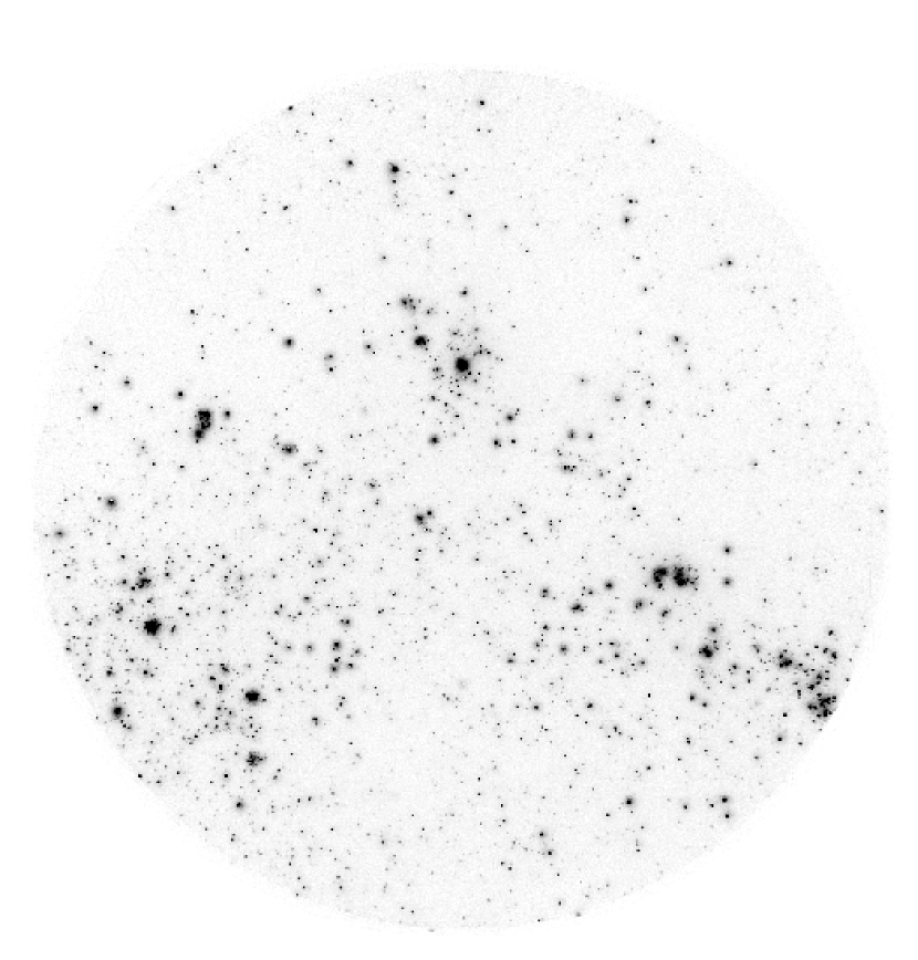
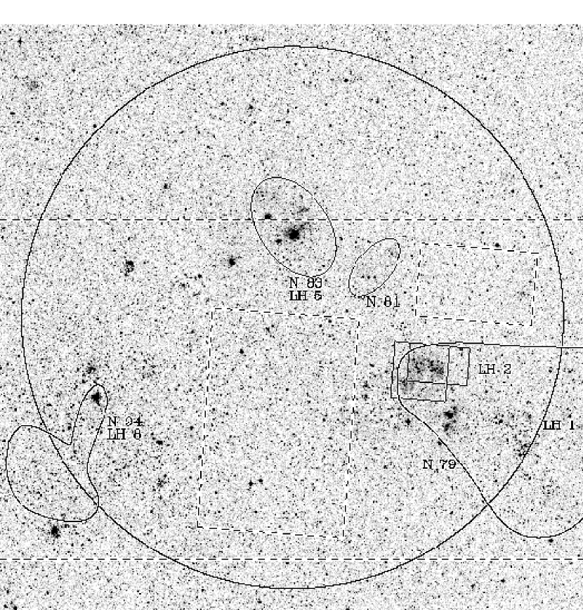
Figure 1: a) The UIT image used in this analysis. b) The the corresponding image from the Digitized Sky Survey. Both images are at the same orientation (north is about 4 degrees clockwise from up, east is to the left) and scale (the UIT image is roughly 37 arcmin in diameter). Several regions are outlined on the Digitized Sky Survey image: the large circle shows the position of the UIT image; the two long, horizontal dashed lines delineate the limits of the field covered by the MCPS; the elliptical and irregular solid outlines indicate Henize (1956) regions; the solid-lined small boxes to the west show the orientation of the CCD images from CTIO85 (rectangular box) and from Oey (1996) (square box) that define the area used in the multi-dataset analysis of the OB association LH 2; and the two larger dash-lined rectangles in the west and the central-south show the “field” regions used to estimate the background field star corrections to the IMF determined from the MCPS data.

The details of the UIT catalog (instrument, observations, and data reduction) are fully discussed by Stecher et al. (1992, 1997) and Parker et al. (1998). During the Spacelab Astro-2 mission which flew aboard the space shuttle Endeavour on 1995 March 2-18, UIT obtained more than 700 ultraviolet images of nearly 200 celestial targets. The images include 16 fields in the LMC and three fields in the SMC (Parker et al., 1998). The UIT observations of the field in Figure 1, designated as “N 79” in the catalog of Parker et al. (1998), were made on 1995 March 14, and consist of two exposures (65 sec, 653 sec) in the B5 filter, which has a centroid wavelength of $\lambda=1615$ Å, and a bandwidth of $\Delta\lambda=225$ Å [see Stecher et al. (1992) for the filter response curve]. The $\sim$37 arcmin diameter photographic images were scanned and digitized with a PDS 1010m microdensitometer, resulting in images with 1.13 arcsec pixels and point-source profiles with FWHM$=3.36\pm 0.29$ arcsec. Calibrations were made in the same manner as for Astro-1 (Stecher et al., 1992), based on laboratory measurements and data obtained during the missions. Flux value zeropoints were derived primarily with comparisons to IUE stars, but also with comparisons to stars observed by OAO-2, HUT, ANS, GHRS, and other UV-capable instruments. UV magnitudes are defined from these fluxes as: $m_{\rm UV}=-2.5\log(F_{\lambda})-21.1.$ Astrometry was performed with reference to HST guide stars (Lasker et al., 1990).

Stellar photometry on the UIT images was performed with idl procedures based on the daophot algorithms (Stetson, 1987). Aperture corrections were calculated for each image, and small corrections were made in the zeropoint offsets so that the median difference of the flux for all stars was zero between the two images (putting both images on the same zeropoint). The final magnitude for each star is the average of its measurements on the two images weighted by the inverse square of its calculated photometric errors. A comparison with IUE observations of three relatively uncrowded stars in the field show that the UIT and IUE fluxes agree to better than 5%. The completeness limits of the ground-based data used in this paper go to slightly later spectral types, so the combined UIT and ground-based dataset is limited by the UV data.

Figure 2 shows the histogram of observed UV magnitudes for the 3533 stars detected in the UIT images of this field. The limiting magnitude is $m_{\rm UV}\approx 17$ mag, the magnitude of an unreddened late B-type ($\sim$ B9) star. The completeness limit, the magnitude to which we should have detected all stars, is $m_{\rm UV}\approx 15$ mag, the magnitude of an unreddened early B-type ($\sim$ B3) star.

Figure 2: The UV ($\lambda=1615$ Å, $\Delta\lambda=225$ Å) luminosity function for all the stars detected in the UIT field (Figure 1a).

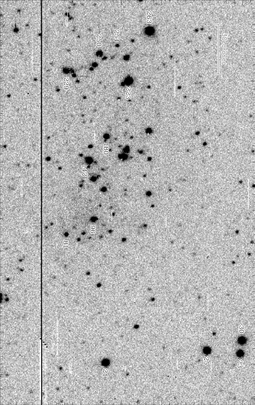
Figure 3: The CCD image from the CTIO85 data (c.f., Figure 1b). North and east are indicated by the arrows. Numbers identify those stars that were observed spectroscopically.

2.2 Ground-based Optical Photometry

The MCPS catalog is discussed by Zaritsky, Harris, & Thompson (1997). The data originate from $UBVI$ drift-scan imaging on the Las Campanas Swope (1 m) telescope with the Great Circle Camera (Zaritsky et al., 1996) and a 2048$\times$2048 pixel CCD with pixel scale of 0.7 arcsec pixel^-1. Typical seeing is $\sim$1.5 arcsec. The data reduction and uncertainties are described in the original paper. The survey is still progressing, so the data presented here are drawn from a preliminary catalog of a small region of the LMC, and for that reason, we do not publish the MCPS data here. (The UIT catalog is already publically available.) The MCPS data for this and other regions will be made public when reductions of nearby regions are complete, and may be superior only in that the overlapping areas between all scans will enable checks and possible corrections to the photometry. As seen in Figure 1b, the currently available scan region does not cover the entire UIT field, so for our UV+optical analysis we can use only this region of overlap. The full scan of this region, obtained in 1997 December, is 124$\times$25 arcmin², resulting in a catalog of 265,794 stars; 80,733 stars are in the region that overlaps with the UIT image. The area of this overlapping region is $\sim$675 arcmin², or 1.4$\times 10^{5}$ pc².

Table 1: The CTIO85 Catalog : Photometry and Astrometry of Stars in LH 2

Star	$\alpha$    (2000.0)    $\delta$		$X$	$Y$	$V$	$\sigma_{V}$	$B-V$	$\sigma_{B-V}$	$U-B$	$\sigma_{U-B}$	O96 ID	Spectral Type
						$\vdots$
81	4:52:00.66	–69:20:49.73	288.80	81.71	15.704	0.014	0.029	0.024	–0.745	0.031	D10b-23	O6 V
82	4:52:00.79	–69:20:39.39	287.52	102.83	16.678	0.030	0.914	0.085	–0.243	0.178	D10b-44
83	4:52:00.96	–69:19:06.23	285.84	293.19	16.844	0.047	1.294	0.109	99.000	9.000	D10b-55
84	4:52:00.98	–69:20:05.92	285.49	171.23	18.717	0.136	–0.179	0.244	99.000	9.000	D10b-308
85	4:52:01.02	–69:20:23.15	284.98	136.02	16.466	0.023	–0.163	0.036	–0.674	0.053	D10b-39
86	4:52:01.06	–69:20:50.53	284.46	80.08	18.927	0.320	–0.665	0.383	99.000	9.000	D10b-504
87	4:52:01.32	–69:18:55.21	282.04	315.71	18.285	1.482	1.363	1.509	99.000	9.000	D10b-500
88	4:52:01.48	–69:21:01.59	279.93	57.46	17.663	0.065	–0.147	0.102	–0.196	0.159	D10b-118
89	4:52:01.50	–69:20:44.84	279.80	91.69	17.864	0.064	–0.077	0.123	–0.751	0.186	D10b-187
90	4:52:01.51	–69:20:04.57	279.70	173.99	18.366	0.107	0.278	0.251	–1.558	0.297	D10b-203
91	4:52:01.69	–69:20:02.02	277.86	179.19	17.038	0.035	–0.166	0.065	–0.596	0.087	D10b-68
92	4:52:01.69	–69:19:40.68	277.85	222.79	18.134	0.081	0.571	0.312	99.000	9.000	D10b-297
93	4:52:01.71	–69:20:26.92	277.61	128.31	18.013	0.074	–0.065	0.138	–0.334	0.244	D10b-181
94	4:52:01.86	–69:20:58.37	275.84	64.04	17.404	0.054	1.222	0.177	99.000	9.000	D10b-105
95	4:52:02.27	–69:20:16.21	271.56	150.19	18.625	0.142	0.353	0.301	–1.225	0.460	D10b-435
96	4:52:02.40	–69:20:33.32	270.12	115.21	14.947	0.019	–0.170	0.024	–0.870	0.023	D10b-12	O7.5 Vz
						$\vdots$

In addition to these two primary datasets, we also use $UBV$ observations from two other sources. One source of $UBV$ data is from observations made by P. Massey and K. DeGioia-Eastwood on 1985 February 12 with the 0.9 m telescope at CTIO. The observed LH 2 field covers an area of 4.1$\times$2.6 arcmin²; the $V$-band CCD image is shown in Figure 3. Details of those observations are given by Massey et al. (1989). The data were reduced with daophot by J.Wm.P. in 1990, and used the transformations to the standard system defined by Massey et al. (1989). The reduction of these LH 2 data was similar to the reductions used in the analyses of other OB associations observed on the same run (e.g., Massey et al., 1989; Massey, Parker, & Garmany, 1989; Parker et al., 1992; Parker, 1993; Garmany, Massey, & Parker, 1994; Oey & Massey, 1995). Astrometric positions were calculated from the CCD X,Y coordinates fitted by daophot and using a plate solution derived with the Grant machine at the offices of the National Optical Astronomical Observatories. A total of 280 stars are in this catalog for LH 2; these data (hereafter: CTIO85) were discussed by Parker, Garmany, & Massey (1990), but had not been published, so for completeness we present them here in Table 1.

Another source of $UBV$ data is from the catalog of Oey (1996); details of the observations (made in 1992 November–December) and data reductions are described therein. A total of 674 stars are in that catalog for LH 2, which covers an area of 3.8$\times$3.8 arcmin². The areas covered by the Oey (1996) and CTIO85 datasets are shown by the rectangular solid outlines in Figure 1b.

2.3 Spectroscopy

UBV photometry alone cannot adequately distinguish O-type from B-type stars (Massey, 1985); Castelli (1999) provides an analysis of the reliability and limitations of $UBV$ photometry to derive stellar effective temperatures ($T_{\rm eff}$). Though UV photometry can help reduce this degeneracy, it still is not as accurate as using spectral types to determine $T_{\rm eff}$ for hot stars. Massey (1998) discusses the utility for UV photometry based on the Hunter et al. (1997) HST UV and optical observations of 30 Doradus. He shows that the inclusion of UV photometry can help better determine $T_{\rm eff}$ for the later-type O stars, but for the hottest, early-type O stars a photometric accuracy of 5% translates to about 1 mag uncertainty in the bolometric correction.

We therefore also have obtained spectroscopic classifications of stars in the LH 2 OB association. We observed the bluest [$Q=(U-B)-0.72\times(B-V)<-0.7$] and brightest ($V<16$ mag) stars in LH 2 based on the CTIO85 photometry, and also observed selected red stars to determine membership and identify foreground stars. Spectra for these stars were obtained on 1991 Jan 29 using the CTIO 4 m telescope and R/C spectrograph with a GEC CCD and the Air Schmidt camera. The KPGL1 grating (632 lines/mm blazed at 4200 Å) was used in first order to obtain a wavelength coverage of 3910–4740 Å. The resolution was $\sim 2.7$ Å (2.0 pixels at 1.3 Å/pixel, which for 22 $\mu$m pixels gives 59 Å/mm). Exposure times longer than about 10 minutes were divided into three separate exposures to allow identification and removal of cosmic rays. These observations were made in conjunction with another observing program (Parker et al., 1992; Parker, 1993), and further details of the observations and reductions can be found therein. The spectra and classifications of the observed early-type stars are shown in Figure 4.

Figure 4: Normalized spectra of the early-type stars in LH 2. Each tick mark on the Y-axis represents 0.25 continuum units.

Classifications were made by comparing observed spectra with: digital spectral standards (Walborn & Fitzpatrick, 1990), standards taken during the run, and all stars observed during the same run (including spectra of other LMC stars for another project) to insure consistency. Walborn (private communication) kindly provided an independent check of the classifications. The earliest type star in the LH 2 OB association is star #81, which is classified as a main-sequence O6 star, implying (along with isochrones fitted to the H-R diagrams discussed in the next section) an approximate cluster age of $\lesssim 3$ Myr, assuming coevality. The nearby star #96 is classified as a O7.5 Vz type; the ZAMS (Vz) luminosity classification based on the relatively deep He II $\lambda$4686 line also implies a young star early in its evolution (Parker et al., 1992; Walborn & Parker, 1992; Walborn & Blades, 1997). Stars #21 and #23 are both classified as O9.7 Ib, and stars #25 and #30, the other visually bright stars in the western region, are both late type stars (spectra were too noisy to classify). Star 254 is clearly a foreground star, with a negligible radial velocity and a very strong Ca II $\lambda$3933 feature. Star 263 was too noisy to classify, but it has very strong Balmer lines, with a velocity consistent with being a Cloud member ($v\sim 210$–260 km s^-1).

These spectra, and the photometry from the sources discussed above, form the datasets with which we analyze in the following sections the stellar populations of the region.

3 COMPARISON AND ANALYSIS OF OPTICAL DATA

From the three optical datasets, we selected those stars that are all within a common, overlapping area. The CCD fields are indicated by the solid, rectangular outlines surrounding LH 2 in Figure 1b, and the overlapping region has an area of $\sim 2.7\times 2.6~{}{\rm arcmin}^{2}\sim 1466~{}{\rm pc}^{2}$. In this area there are 222 stars from the CTIO85 catalog, 387 stars from the Oey (1996) catalog, 667 stars from the MCPS catalog, and 50 stars from the UIT catalog. These differences in the number of stars are primarily due to different exposure times and limiting magnitudes, but a detailed comparison also shows that in some cases there were also differences in identification of close multiples, e.g., objects that were identified as multiple stars in one dataset were identified as only one star in another.

Figure 5 shows the magnitude distribution of the three optical datasets. The completeness magnitudes for CTIO85, Oey (1996), and the MCPS are roughly $V\sim 18$, 18.5, and 19.5 mag, respectively. These magnitudes are the values we will use in the following analysis and determination of the valid mass range for the IMF calculations.

Figure 5: A comparison of the $V$-filter observed magnitude distributions of the three ground-based datasets.

Table 2: Comparison of $Q$ Indexes for Stars with Known Spectral Types

Star	Spectral Type	$Q_{\rm Spec}$	$Q_{\rm MCPS}$	$Q_{\rm CTIO85}$	$Q_{\rm O96}$
21	O9.7 Ib	$-1.11$	$-0.64\pm 0.12$	$-0.81\pm 0.04$	$\cdots$
23	O9.7 Ib	$-1.11$	$-0.77\pm 0.08$	$-0.91\pm 0.11$	$\cdots$
81	O6 V	$-0.95$	$-1.09\pm 0.11$	$-0.77\pm 0.04$	$-0.93\pm 0.02$
96	O7.5 Vz	$-0.93$	$-0.63\pm 0.09$	$-0.75\pm 0.03$	$-0.82\pm 0.01$
142	O7 II:	$-0.91$	$-0.71\pm 0.07$	$-0.61\pm 0.02$	$-0.89\pm 0.01$
180	O9.5 V	$-0.88$	$-0.77\pm 0.08$	$-0.76\pm 0.06$	$-0.86\pm 0.01$
223	O8 II((f))	$-0.91$	$-0.77\pm 0.61$	$-0.60\pm 0.01$	$-0.87\pm 0.01$
229	O9.5 V:	$-0.88$	$-1.02\pm 0.10$	$-0.90\pm 0.04$	$-0.70\pm 0.03$
250	O7 V	$-0.94$	$-0.81\pm 0.16$	$-0.74\pm 0.03$	$-0.90\pm 0.01$
		$\Delta Q=$	$0.17\pm 0.18$	$0.27\pm 0.07$	$0.05\pm 0.05$

Figure 6 shows a comparison of the magnitudes of stars in the LH 2 region from the MCPS data and results from CTIO85 and Oey (1996). The $V$ and $B$ data from CTIO85 are in reasonable agreement (within a few percent) with the MCPS data, though there is a significant, 20% zeropoint offset in the $U$ photometry. A comparison with the Oey (1996) data shows comparable scatter, but 10–15% offsets in all three filters. For an independent comparison of the photometry of the three datasets, in Table 2 we compare the observed colors to the spectroscopically-calibrated colors of the early type stars for which we have classified spectra (Figure 4). The Oey (1996) data show a good agreement on average with the spectroscopic calibrations, and the MCPS and CTIO85 data show offsets of about 20% and 30%, respectively, with fairly large scatter. This is consistent with the comparisons shown in Figure 6. Such large, systematic differences cannot be due to, e.g., incorrect values for the reddening slope or intrinsic colors for LMC stars, since the same values were used for all three datasets. A probable culprit could be the aperture corrections that were adopted in the original reduction of each dataset; the corrections likely are the largest potential source of error in the photometric calibrations.

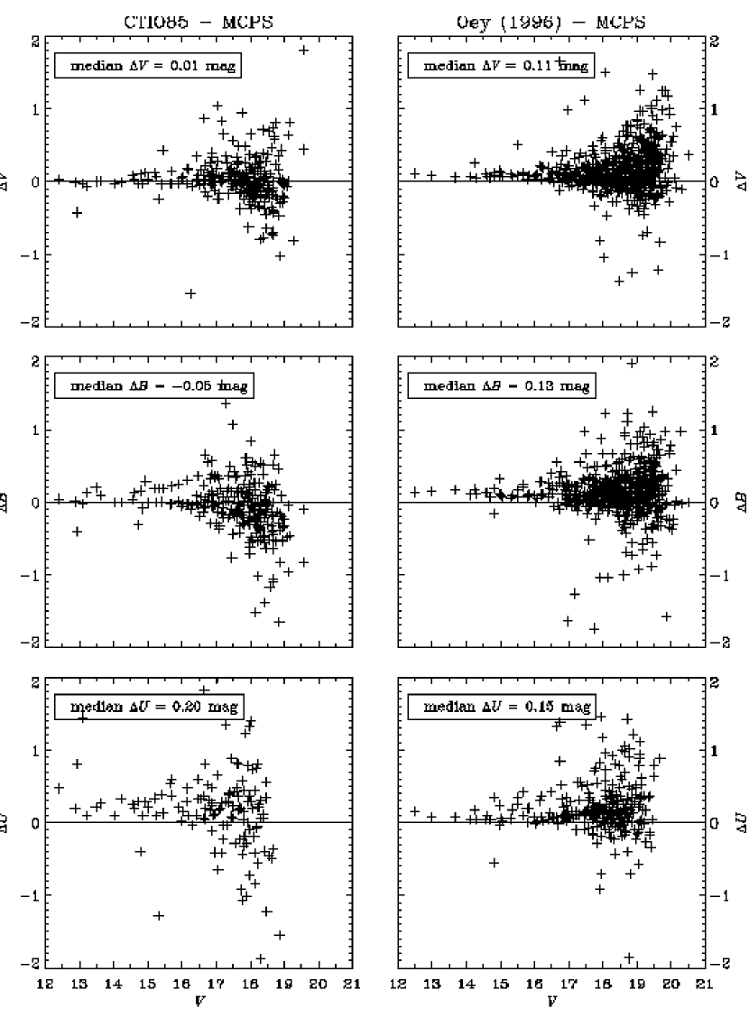
Figure 6: Left column: A comparison of the photometry from the MCPS and unpublished photometry from CTIO85 in the sense of CTIO85 $-$ MCPS. Right column: A similar comparison between photometry from the MCPS and Oey (1996).

To calculate effective temperatures ($T_{\rm eff}$), bolometric corrections, bolometric magnitudes ($M_{\rm bol}$), masses, and IMFs, we follow the general method used by Massey et al. (1989) and numerous subsequent studies of OB associations in the Magellanic Clouds (e.g., Massey, Parker, & Garmany, 1989; Massey et al., 1995; Parker et al., 1992; Parker & Garmany, 1993; Walborn et al., 1999). In outline: first, a typical reddening, $E(B-V)_{t}$, is determined for the association. Then, for “blue” stars [stars having $-0.96<Q<-0.40$, or with both $-0.40<Q<0$ and $(B-V)_{0}=(B-V)-E(B-V)_{t}<0$], the $T_{\rm eff}$ is calculated from their $Q$ index, and for other stars from their intrinsic $(B-V)_{0}$ colors. The bolometric correction is calculated from the $T_{\rm eff}$, and the resulting $T_{\rm eff}$-$M_{\rm bol}$ values are plotted on the Hertzsprung-Russell diagram (HRD). We use the Geneva evolutionary models (Schaerer et al., 1993; Meynet et al., 1994) with a metallicity of $Z=0.008$ to then bin the stars on the HRD by mass to determine the ZAMS mass for each star, and thereby calculate an IMF. The next few paragraphs describe our particular steps in more detail.

To estimate $E(B-V)_{t}$ for the LH 2 region, we used three methods for each dataset: (i) we estimated by eye the reddening necessary to “slide” the observed color-magnitude diagrams to the intrinsic ZAMS color-magnitude relationship; (ii) we use the $Q$ index for various subsets of the bluest stars to calculate the typical reddening; and (iii) we compared the observed and intrinsic $B-V$ colors for the stars that have spectroscopic classifications. All the datasets were in reasonable agreement, giving an average value of $E(B-V)_{t}=0.20\pm 0.02$ s.d.m., and a median value of $E(B-V)_{t}=0.16$ (although the standard deviation of the mean is small, the range of $E(B-V)$ values was quite large, with standard deviations typically $\pm 0.15$, most likely due to intrinsic reddening variations within the field). This value is slightly larger than but consistent with results from other analyses (Lucke, 1972, 1974; Ye, 1998); those studies also find that LH 2 has an extinction larger than typical for LMC associations.

For the special cases of stars with known spectral types, the reddenings were determined from the intrinsic colors of Johnson (1966), and their $T_{\rm eff}$ were determined using the calibrations of Vacca, Garmany, & Shull (1996) and Humphreys & McElroy (1984). For other “blue” stars ($Q<-0.2$), the reddening and $T_{\rm eff}$ were calculated from their $Q$ index. For the remaining stars, the median typical reddening value of $E(B-V)_{t}=0.16$ was used, and $T_{\rm eff}$ was calculated from $(B-V)_{0}$. For all stars, the bolometric correction was calculated from $T_{\rm eff}$.

Figure 7: The theoretical HRDs for the three ground-based datasets. The symbols indicate: stars with determined spectral types (filled circle, $\bullet$), stars with photometry only and all uncertainties in $UBV<0.07$ mag (open circles, $\circ$), and stars with photometry only and at least one uncertainty $>0.07$ mag (crosses, +). The “blue plume” of stars to the left of the ZAMS is an artifact of large errors for the fainter stars, as discussed in the text.

The resulting $M_{\rm bol}$ and $T_{\rm eff}$ values for each dataset were plotted on the HRD. Figure 7 shows the HRDs for the data, overplotted with the evolutionary tracks of Schaerer et al. (1993) for Z = 0.008. Stars with determined spectral types are plotted with filled circles, stars with photometry only and all uncertainties in $UBV<0.07$ mag are plotted with open circles, and stars with an uncertainty of $>0.07$ mag in at least one filter are plotted with crosses. The “blue plume” of stars to the left of the ZAMS is a feature seen in nearly all previous similar studies. This feature is primarily due to faint stars with large uncertainties; in particular, erroneously too-bright $U$ and/or $B$ magnitudes result in incorrectly large calculated $T_{\rm eff}$ and bolometric corrections. As seen when comparing the plots in Figure 7, these stars mostly disappear once a cutoff magnitude consistent with the completeness magnitudes is used. Only the MCPS dataset still has a significant number of blue plume stars, perhaps indicating larger photometric errors relative to the magnitude limit.

Figure 8: The IMFs for the three ground-based datasets: a) CTIO85, b) Oey (1996), c) MCPS, d) MCPS after field star correction. In all cases, the solid line indicates an unweighted fit to the data points indicated by the filled symbols, and the dashed line indicates a fit weighted by the number of stars in each bin (in most cases, the fits indicated by the dashed and solid lines are nearly indistinguishable). The circles indicate all stars in each dataset. In panels a–c, the crosses ($\times$) indicate those stars that are brighter than the completeness magnitude cutoff determined for each dataset (c.f. Figure 5). For panel d, the triangles indicate the MCPS data for LH 2 after the estimated field star contribution has been removed.

The resulting IMFs for the data are shown in Figure 8. These IMFs include all the stars to the right of the ZAMS shown in the HRDs in Figure 7. We have not included all the extant stars in the blue plume in the IMF calculation since their true locations in the HRD are unknown but are likely to be in the lower mass bins; however, to allow for some real uncertainty in $T_{\rm eff}$, we do include in the IMF those stars with $T_{\rm eff}$ up to 0.05 dex to the left of the ZAMS. Also, no correction has been made for the evolved stars (e.g, the star between the 12 and 15 ${\cal M}_{\odot}$ mass tracks near $\log\mbox{$T_{\rm eff}$}\sim 3.8$), which are few in number so they do not have a significant effect on the IMF slope. The fairly narrow main sequence in the HRDs implies that our assumption of coevality of this association is reasonable.

The IMF slopes for the full datasets (panels a–c in Figure 8) are in remarkable agreement, in spite of the differences seen in the photometry and the appearance of the HRDs. However, we would like to emphasize two points: all these IMFs rely on the same spectroscopic classifications for the bluest, most massive stars, which reduces any effects from photometric differences; and clearly it is possible to get similar or even “correct” IMF slopes fortuitously with data that have large uncertainties. Massey (1998) points out that a systematic error in $M_{\rm bol}$ (due to, e.g., errors in the photometry, calibrations, or adopted distance modulus) does not change the slope of the IMF; the stars tend to shift uniformly from one bin to another without necessarily changing the slope of the IMF.

Table 3: Stars with Spectroscopic Observations

				$T_{\rm eff}$ (K)				$E(B-V)$
Star	$\alpha$    (2000.0)    $\delta$		Spectral Type	spec	photQ	phot		spec	photQ	phot	match
21	4:51:45.98	–69:20:25.9	O9.7 Ib	30500	17000	23000		0.01	–0.04	0.10	0.19
23	4:51:47.05	–69:19:04.3	O9.7 Ib	30500	22000	27000		0.10	0.09	0.19	0.21
25	4:51:47.39	–69:19:24.5	late type	$\cdots$	$\cdots$	$\cdots$		$\cdots$	$\cdots$	$\cdots$	$\cdots$
30	4:51:48.55	–69:19:03.3	late type	$\cdots$	$\cdots$	$\cdots$		$\cdots$	$\cdots$	$\cdots$	$\cdots$
81	4:52:00.66	–69:20:49.7	O6 V	43560	50000	42500		0.28	0.32	0.28	0.28
96	4:52:02.40	–69:20:33.3	O7.5 Vz	39730	17000	26000		–0.02	–0.11	0.07	0.17
142	4:52:09.12	–69:20:35.7	O7 II:	39290	20000	26000		0.06	–0.01	0.10	0.20
180	4:52:11.88	–69:20:25.2	O9.5 V	34620	26000	30000		0.08	0.05	0.11	0.13
223	4:52:18.22	–69:20:11.7	O8 II((f))	37090	22000	19000		0.13	0.09	0.01	0.22
229	4:52:19.32	–69:20:49.3	O9.5 V:	34620	50000	24000		0.46	0.51	0.07	0.17
250	4:52:21.34	–69:20:29.4	O7 V	41010	28000	40000		0.17	0.13	0.21	0.22
254	4:52:22.26	–69:20:18.6	foreground	$\cdots$	$\cdots$	$\cdots$		$\cdots$	$\cdots$	$\cdots$	$\cdots$
263	4:52:23.96	–69:19:58.9	LMC member	$\cdots$	$\cdots$	$\cdots$		$\cdots$	$\cdots$	$\cdots$	$\cdots$

The MCPS data have the advantage that they cover sufficient area to allow correction for contamination of background stars (i.e., LMC field stars) in the area of LH 2. We selected two large fields (indicated by the dashed-lined boxes in Figure 1b) by eye to serve as background fields. Stars in these fields were run through the same calculations to determine IMF masses. The number of stars in each mass bin was scaled by the relative sizes of the LH 2 and the background fields, and then was subtracted from the IMF plotted in Figure 8c. The resulting field star corrected IMF is shown in Figure 8d. This IMF is notably flatter than the uncorrected IMF. The fact that field stars can affect the observed IMF is not a new idea, but it is a correction that is often not made, possibly because most observations do not cover a large enough area to make the measurement and correction and it is assumed that there are not many or sufficient OB-type field stars to bias the sample. Our result simply emphasizes the fact that this correction is important even for OB-type stars, and, if the IMF slope is constant and universal, such field contamination could possibly even be a major factor causing the wide range of observed IMF slopes.

4 ANALYSIS OF UIT AND MCPS DATA

4.1 Determination of Reddening and Effective Temperatures

The UIT data were combined with the MCPS data using all MCPS stars within the field-of-view of the UIT image, which contains 80733 stars from the MCPS catalog and 3533 stars in the UIT catalog. Because the MCPS data do not extend across the entire declination range of the UIT field (see Figure  1b), we will only use the overlapping sub-region for our analysis in this paper. In that region, there are 2770 MCPS stars that have UV photometry from the UIT catalog. These stars were matched by positional coincidence with a 3 arcsec tolerance.

To compare our photometry to Kurucz (1992, 1993) models, we use UV and optical magnitudes derived from filter functions convolved with Kurucz spectra. The UV magnitudes were derived by Landsman (personal communication) by convolving Kurucz spectra with the UIT response curve. Optical/IR standard broad band colors and magnitudes for the Kurucz models were calculated by Bessell, Castelli, & Plez (1998); however, those data were determined for solar abundances. From those authors we obtained their data for models with $[M/H]=-0.5$, more appropriate for LMC metallicity (Kontizas et al., 1993).

Figure 9: The number distribution of effective temperatures ($T_{\rm eff}$) determined by fitting the UV and optical photometric data and allowing the $E(B-V)$ reddening to be a variable of the fit for each star.

The observed magnitudes were compared to the synthetic photometry of the models to determine the best matching model ($T_{\rm eff}$ and surface gravity) using a number of different programs and best-fit estimators. In Table 3 we show the results of some of these fits for those stars that have spectroscopic observations, and therefore, good estimates of their true $T_{\rm eff}$. In one case (the “phot_Q” columns), we first calculated the $E(B-V)$ for each star using the $Q$ index as determined from the $UBV$ photometry (Table 2), dereddened the observed colors, then performed the fit of the data to the models. In another case (the “phot” columns) we allowed $E(B-V)$ to be a free parameter in the fit. For comparison, in the “spec” columns, we also show the $E(B-V)$ calculated from the observed $B-V$ color and the intrinsic $(B-V)_{0}$ color based on the color vs. spectral type calibration. In all cases, for the reddening law we use the functional form of Fitzpatrick & Massa (1986, 1988) with the “average LMC” coefficients derived by Misselt, Clayton, & Gordon (1999), and fits were weighted using the daophot-derived photometric errors. (In many cases for the COTS, the $I$ data were saturated, which is reflected in the quoted errors.)

In nearly all cases, the $T_{\rm eff}$ calculated in the fit underestimates the “true” $T_{\rm eff}$ as determined from calibration with spectral type (Vacca, Garmany, & Shull, 1996), though about half have reasonably good fits (i.e., the difference in $T_{\rm eff}$ is $<0.1$ dex). In the “match” column of Table 3 we show the $E(B-V)$ that would be required to get the fitted $T_{\rm eff}$ to match the spectroscopic $T_{\rm eff}$. If the calculated $Q$ is too red, the resulting $E(B-V)$ and $T_{\rm eff}$ values will also be too low. If we adjust the MCPS data by the value of $\Delta Q=0.17$ shown in Table 2, the fitted $T_{\rm eff}$ values are significantly improved, but still too low on average. It is probably the case that this systematically too-low $T_{\rm eff}$ is not only a factor of an incorrectly derived reddening, but possibly also due to a model calibration error; the fits are most sensitive to the UV–optical colors, which involve two different photometric systems that may not be well cross-calibrated. However, we should point out that if we use only the optical data to calculate $E(B-V)$ and/or perform the fit, the fitted $T_{\rm eff}$ values even further underestimate the true temperatures in most cases, so the addition of the UV data, while not a sufficient replacement for getting spectral types, definitely improves our estimate of $T_{\rm eff}$ for O-type stars. So although the inclusion of the UV data does not allow us to definitively identify the O-type stars and determine their $T_{\rm eff}$, it allows us to establish a better lower limit to the number of O-type stars in the catalog than optical data would alone.

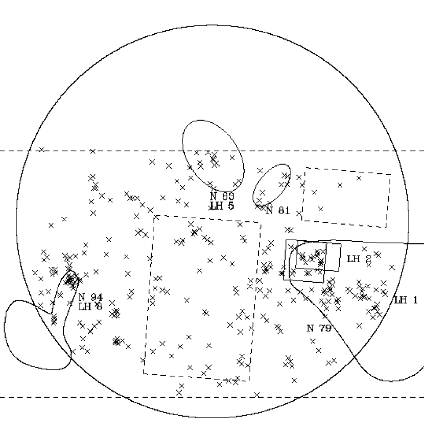
Figure 10: The spatial distribution stars with $\mbox{$T_{\rm eff}$}\geq 30,000$ K determined by fitting the UV and optical photometric data as discussed in the text. The outlines indicate the same regions shown in Figure 1b.

We then performed these fits to all 2770 stars in our dataset that have UV and optical data, and the temperature distribution is shown in Figure 9. The qualitative shape of the distribution is roughly as expected: it rises up quickly at low $T_{\rm eff}$ (due to incompleteness and observational bias against the fainter, cooler stars), then the numbers steadily decrease going to higher $T_{\rm eff}$, reflective of the IMF. There are two unusual features: a plateau (and small spike) between 26,000 and 30,000 K, and a spike at $T_{\rm eff}$ = 50,000 K. It is unclear if these are artifacts of the fit or real features. For example, the spike at 50,000 K could be because that is the maximum $T_{\rm eff}$ in the models, so all hotter stars are put into that bin. Also, another point of concern is that we find a slight trend of hotter stars having larger $E(B-V)$ values on average (although there is a large scatter; stars of all temperatures do show a wide range of reddenings). Since the reddening is a variable in the fit, if the reddening is overestimated for a star, then the $T_{\rm eff}$ may be overestimated. However, a similar though less steep trend is seen if one compares the $E(B-V)$ derived purely from the $UBV$ photometry via the $Q$ index. So this trend may be real, and may reflect the situation that the hottest, most massive stars also are the shortest-lived, and therefore are more likely to still be in or near their birth regions, which will have larger than average extinction. In fact, the $Q$-derived $E(B-V)$ values tend to be larger on average than the fitted values (contrary to the trend seen with the few stars in Table 3); if the reddening values are, indeed, larger than the fitted values, then our $T_{\rm eff}$ estimates may be too low, and there may be more stars with higher temperatures than shown in Figure 9.

4.2 Candidate O-type Stars

Taking our results at face value, there are 322 stars with $\mbox{$T_{\rm eff}$}\geq 30,000$ K, the typical temperature of the latest O-type star. We note that the comparison in Table 3 and the previous discussion about the reddening imply that our fits may tend to underestimate the true temperatures. In Table 3, O-type stars have fitted temperatures as low as $\sim$20,000 K. We find 1820 stars with fitted $\mbox{$T_{\rm eff}$}\geq 20,000$ K. Given that the area of the dataset is $\sim$1.4$\times 10^{5}$ pc², these numbers translate to a density of one O-type star per $\sim$80–430 pc² (0.4–2.1 arcmin²). For comparison, the density in the solar neighborhood is less one O-type star per 40,000 pc² (Garmany, Conti, & Chiosi, 1982).

Figure 10 shows the spatial distribution of the stars with $\mbox{$T_{\rm eff}$}\geq 30,000$ K in the region we analyzed. Note the large number of COTS well-distributed outside of the boundaries of the classical OB associations: about 200 of the hot stars, nearly two-thirds of the COTS, are outside the boundaries of the “N” and “LH” regions shown in Figure 10. How many of these may be true field stars? Massey et al. (1995) define “field stars” as those that are farther from the boundary of any OB association than the distance an O-type star could travel in its lifetime (10 Myr for late-type O stars) at a typical dispersion velocity of $\sim 3$ km s^-1 relative to the parent molecular cloud. This distance is about 30 pc, or 2 arcmin at the distance of the LMC. This is a reasonable definition for most cases. If we count only those stars beyond $\sim$2 arcmin from any of the boundaries, that still leaves about 160 stars. Approximately equal numbers of COTS are found in the field and in OB associations. This result is in accord with earlier suggestions from the Galactic study of Garmany, Conti, & Chiosi (1982); their Figure 2 shows that perhaps the majority of the O stars within 3 kpc of the Sun are not in OB associations. Our result can be extrapolated to the general distribution of massive stars in the LMC only if one assumes that the region studied here is large enough to provide a representative and proportional sample of field and association areas. The density of “field” OB stars in this region is roughly one star per 700 pc² (3.5 arcmin²).

Because of the uncertainties in obtaining $T_{\rm eff}$ from photometry alone, these estimates will have to be verified with spectroscopic observations. It is unclear if our estimates of the O-type star population may be high or low: some of these COTS will turn out to be later-type stars because we have over-estimated their $T_{\rm eff}$, but it is perhaps even more likely that there were many O-type stars that were missed because we under-estimated their $T_{\rm eff}$ (e.g., as in Table 3, many O-type stars were fitted $\mbox{$T_{\rm eff}$}<30,000$ K). Also, because we have only considered those stars with both UV and optical photometry, some O-type stars may have been missed in our analysis because they were too heavily obscured to be detected in the UV, and this may be a stronger effect in the younger star forming regions where extinction is higher. In light of these uncertainties, our analysis has been reasonably conservative, and we conclude that our results provide a lower limit to the total population of O-type stars in the field.

5 SUMMARY

In this paper we have analyzed the UV photometric data from UIT along with the optical ($UBVI$) data from the Magellanic Cloud Photometric Survey and other ground-based sources to study the stellar content within and near N 79 in the southwest region of the LMC. Our analysis of these data gives the following results:

• Comparisons of three different optical datasets for the LH 2 OB association show that although the datasets exhibit median photometric differences of up to 30%, the resulting observed, uncorrected IMFs are reasonably similar, typically $\Gamma\sim-1.6$ in the 5–60 ${\cal M}_{\odot}$ mass range.

• When we correct for the background contribution of field stars in the one dataset where this is possible, the calculated IMF flattens to $\Gamma=-1.3\pm 0.2$ (similar to the Salpeter IMF slope). This implies that the background contribution of stars—even for massive stars—may be an important factor to the range of IMF slopes found in the literature.

• Fitting the UV+optical data to Kurucz models, we find 322 stars with fitted $\mbox{$T_{\rm eff}$}\geq 30,000$ K (the lower limit for $T_{\rm eff}$ for a typical, latest type O star), and 1820 stars with fitted $\mbox{$T_{\rm eff}$}\geq 20,000$ K (the lower limit for the fitted $T_{\rm eff}$ for known O-type stars used for comparison in Table 3).

• We find evidence that the number of candidate O-type “field” stars is roughly equal to the number of such stars in OB associations. This distribution is very interesting in that it provides strong confirmation of the conventional wisdom; see Garmany, Conti, & Chiosi (1982).

This work shows the potential of the large-scale analysis of stellar populations that will be possible when the MCPS is complete and combined with the UIT dataset. The results of this and similar studies are leading us to make more detailed observations of the massive star content of the field region in both Magellanic Clouds to better understand the origin of these stars and their IMF. We are presently conducting spectroscopic observations and further analysis to determine if these are true isolated field stars, not born in OB associations, or if they are high-velocity runaways or members of many previously unrecognized, low-density OB associations. We will also include field regions of the LMC and SMC that are notably less active in present star formation (e.g., farther from or containing fewer and smaller OB associations) to see if our results here are representative of the global distribution of massive stars. Ultimately, these data will allow us to resolve discrepant measurements of the field star IMF and the origins of massive stars. If there is a significant population of massive field stars that have formed in situ as isolated events, it will have important implications on concepts and models of star formation.

References

- Bessell, Castelli, & Plez (1998) Bessell, M.S., Castelli, F. & Plez, B. 1998, A&A, 333, 231
- Castelli (1999) Castelli, F. 1999, A&A, 346, 564
- Elmegreen (1997) Elmegreen, B.G. 1997, ApJ, 486, 944
- Elmegreen (1999a) Elmegreen, B.G. 1999a, ApJ, 515, 323
- Elmegreen (1999b) Elmegreen, B.G. 1999b, in The Evolution of Galaxies on Cosmological Timescales, eds. J.E. Beckman and T.J. Mahoney (San Francisco, ASP), 145
- Elmegreen (2000) Elmegreen, B.G. 2000 MNRAS, 311, L5
- Elmegreen & Hunter (2000) Elmegreen, B.G., & Hunter, D.A. 2000, ApJ, 540 814
- Fitzpatrick & Massa (1986) Fitzpatrick, E.L. & Massa, D. 1986, ApJ, 307, 286
- Fitzpatrick & Massa (1988) Fitzpatrick, E.L. & Massa, D. 1988, ApJ, 328, 734
- Garmany, Conti, & Chiosi (1982) Garmany, C.D., Conti, P.S., & Chiosi, C. 1982, ApJ, 263, 777
- Garmany, Massey, & Parker (1994) Garmany, C.D., Massey, P., & Parker, J.Wm. 1994, AJ, 108, 1256
- Harris, Zaritsky, & Thompson (1997) Harris, J., Zaritsky, D., & Thompson, I. 1997, AJ, 114, 1933
- Henize (1956) Henize, K.G. 1956, ApJS, 2, 315
- Hodge & Wright (1977) Hodge, P.W., & Wright, F.W. 1977, The Small Magellanic Cloud, (University of Washington Press, Seattle)
- Humphreys & McElroy (1984) Humphreys, R.M., & McElroy, D.B. 1984, ApJ, 284, 565
- Hunter et al. (1997) Hunter, D.A., Vacca, W.D., Massey, P., Lynds, R., & O’Neil, E.J. 1997, /ap, 113, 1691
- Johnson (1966) Johnson, H.L. 1966, ARA&A, 4, 193
- Kontizas et al. (1993) Kontizas, M., Kontizas, E., & Michalitsianos, A. G. 1993, A&A, 269, 107
- Kurucz (1992) Kurucz, R.L. 1992, in IAU Symp. 149, The Stellar Populations
- Kurucz (1993) Kurucz, R.L. 1993, CD-ROM No. 13 of Galaxies, eds. B. Barbuy & A. Renzini (Dordrecht: Kluwer), p. 255
- Lasker et al. (1990) Lasker, B. M., Sturch, C. R., Mclean, B. J., Russell, J. L., Jenkner, H. 1990, AJ, 99, 219
- Leitherer et al. (1996) Leitherer, C. et al. 1996, PASP, 108, 996
- Lucke (1972) Lucke, P.B 1972, Ph.D.thesis, University of Washington
- Lucke (1974) Lucke, P.B 1974, ApJS, 28, 73
- Lucke & Hodge (1970) Lucke, P.B., & Hodge, P.W. 1970, AJ, 75, 171
- Massey (1985) Massey, P. 1985, PASP, 97, 5
- Massey (1998) Massey, P. 1998, in The Stellar Initial Mass Function, 38th Herstmonceux Conference, ed. Gilmore & Howell (San Francisco, ASP), 17
- Massey et al. (1989) Massey, P., Garmany, C.D.,Silkey, M., & Degioia-Eastwood, K. 1989, AJ, 97, 107
- Massey et al. (1995) Massey, P., Lang, C.C., DeGioia-Eastwood, K, & Garmany, C.D. 1995, ApJ, 438, 188
- Massey, Parker, & Garmany (1989) Massey, P., Parker, J. W. & Garmany, C. D. 1989, AJ, 98, 1305
- Melnick & Selman (2000) Melnick, J., & Selman, F. 2000, in Cosmic Evolution and Galaxy Formation; Structure, Interactions, and Feedback, ed. Franco, Terlevich, López-Cruz, and Atetxaga (San Francisco, ASP), in press
- Meynet et al. (1994) Meynet, G., Maeder A., Schaller G., Schaerer D., & Charbonnel C. 1994, A&AS, 103, 97
- Misselt, Clayton, & Gordon (1999) Misselt, K.A., Clayton, G.C., & Gordon, K.D. 1999, ApJ, 515, 128
- Oey (1996) Oey, M.S. 1996, ApJS, 104, 71
- Oey & Massey (1995) Oey, M.S., & Massey, P. 1995, ApJ, 452, 210
- Parker (1993) Parker, J.Wm. 1993, AJ, 106, 560-577
- Parker & Garmany (1993) Parker, J.Wm. & Garmany, C.D. 1993, AJ, 106, 1471
- Parker et al. (1996) Parker, J.Wm. et al., 1996, ApJ, 472, L29
- Parker et al. (1998) Parker, J.Wm. et al., 1998, AJ, 116, 180
- Parker, Garmany, & Massey (1990) Parker, J.Wm., Garmany, C.D., & Massey, P. 1990, BAAS, 22, 1290
- Parker et al. (1992) Parker, J.Wm., Garmany, C.D., Massey, P. & Walborn, N.R. 1992, AJ, 103, 1205
- Richtler (1994) Richtler, T. 1994, A&A, 287, 517
- Salpeter (1955) Salpeter, E.E. 1955, ApJ, 121, 161
- Stecher et al. (1992) Stecher, T. P., et al. 1992, ApJ, 395, L1
- Stecher et al. (1997) Stecher, T. P., et al. 1997, PASP, 109, 584
- Schaerer et al. (1993) Schaerer, D., Meynet, G., Maeder, A., & Schaller, G. 1993, A&AS, 98, 523
- Stetson (1987) Stetson, P. B. 1987, PASP, 99, 191
- Vacca, Garmany, & Shull (1996) Vacca, W.D., Garmany, C.D., & Shull, J.M. 1996, ApJ, 460, 914
- Walborn & Blades (1997) Walborn, N.R. & Blades, J.C. 1997 ApJS, 112, 457
- Walborn et al. (1999) Walborn, N.R., Drissen, L., Parker, J.Wm., Saha, A., MacKenty, J.W., & White, R.L. 1999, AJ, 118, 1684
- Walborn & Fitzpatrick (1990) Walborn, N.R. & Fitzpatrick, E.L. 1990, PASP, 102, 379
- Walborn & Parker (1992) Walborn, N.R., & Parker, J.Wm. 1992, ApJ, 399, L87
- Ye (1998) Ye, T. 1998 MNRAS, 294, 422
- Zaritsky et al. (1996) Zaritsky, D., Shectman, S.A., & Bredthauer, G. 1996, PASP 104, 108
- Zaritsky, Harris, & Thompson (1997) Zaritsky, D., Harris, J., & Thompson, I. 1997, AJ, 114, 1002