Protoneutron star in the Relativistic Mean-Field Theory

Abstract

In this review the basic properties of nonrotating and slowly rotating protoneutron stars in the relativistic mean-field approach are discussed. The equation of state is the main input to the structure equations. The TM1 parameter set extended to the case of finite temperature is used to obtain the mass-radius relation for protoneutron stars. The occurrence of unstable areas in the mass-radius relation are presented. This allows for the existence of distinctively different evolutionary of tracks of the protoneutron stars. The low density protoneutron star configurations are estimated. The obtained stable configurations for the fixed lepton number $Y_{L}=0.4$ are compared with ones obtained for the fixed proton fraction $Y_{P}=0.1776$.

1 Introduction

Protoneutron star is a hot, lepton-rich neutron object which is formed in Type-II supernovae explosion as the final stage of a star more massive than about 8 $M_{\odot}$ - 25 $M_{\odot}$ [1]. The evolution of a protoneutron star depends on two factors: the relativistic equation of state of the stellar matter and neutrino interactions which provide to the phenomena of neutrino trapping in a neutron star matter . Neutrino interactions play a crucial role during the creation of the protoneutron star. At the beginning, this star is very hot and lepton-rich, after a typical time of several tens of seconds, the star becomes cold, deleptonized object and the neutron star is formed. During the collapse enormous energy of the order of $\sim 10^{53}$ ergs is released just through neutrinos. The released energy is equal to the gravitational binding energy of a newly formed neutron star. In this paper the mass-radius relation of the protoneutron star is constructed for different temperature cases. A particularly interesting situation results in the occurrence of unstable areas which allows distinctively different evolutionary tracks. In the new-born protoneutron star (less than several seconds) neutrinos are trapped locally in the dense stellar matter at densities greater than $10^{13}$ $g/cm^{3}$, forming an ultrarelativistic and degenerate Fermi gas. This trapped neutrinos have an influence on the equation of state [1, 2, 3, 4, 5].
The outline of this paper is as follows.
In Sect.1 the general properties of nonrotating and rotating protoneutron stars are calculated. In Sect.2 the employed equation of state is obtained in the approach of relativistic mean-field approximation. This approach imply the nucleons interactions through the exchange of meson fields. Thus the model considered here comprises: electrons, muons, neutrinos and scalar, vector-isoscalar and vector-isovector mesons. Consequently the pressure and energy density are characterized by contributions coming from these components. In Sect.3 the influence of rotation on the protoneutron stars parameters such as: masses, radii and moment of inertia are calculated. The obtained results for the given form of the equation of state followed by a discussion of the implications of these results are presented in Sect.4 and Sect.5.
In this article the signature $\{-,+,+,+\}$ is used, in which the Dirac’s matrix is defined by

$$\{\gamma^{\mu},\gamma^{\nu}\}=-2g^{\mu\nu}I.$$

and

$$\Box=\partial_{\mu}\partial^{\mu}=\triangle-\frac{\partial^{2}}{\partial t^{2}}$$

and $\hbar=c=1$. In case of the fermion fields it is more convenient to use the reper field $e^{a}_{\mu}$ defined as follows $g_{\mu\nu}=e^{a}_{\mu}e^{b}_{\nu}\eta_{ab}$ where $\eta_{ab}$ is the flat Minkowski space-time matrix.

2 The theoretical model

This paper presents a basic model of a protoneutron star in the RMF approximation [6, 7, 8, 9, 10]. The relativistic approach to high-density nuclear matter in this approach was proposed by Walecka. Since then, this theory has been applied successfully to many subjects in nuclear many body problems. Especially the Walecka model (QHD) and its nonlinear extensions have been quite successfully and widely used for the description of hadronic matter and finite nuclei. Increasing interest in the neutron star matter at finite temperature has been observed recently in relation to the problems of hot neutron stars and protoneutron stars and their evolution in particular. Theories concerning protoneutron stars are being discussed in works by Prakash et al. [1, 2, 4, 11, 12, 13]. Glendenning [14] has studied the properties of neutron star in the framework of nuclear relativistic field theory. In the field theoretical approach the nuclear matter is described as the baryons interaction through mesons $\sigma$, $\omega$ and $\rho$ exchange. We define an action of the protoneutron star through the Lagrangian density ${\mathcal{L}}$

$$S=\int d^{4}x\sqrt{-g}{\mathcal{L}}.$$ (1)

The Lagrangian density function of this theory can be represented as the sum

$${\mathcal{L}}={\mathcal{L}_{B}}+{\mathcal{L}_{L}}+{\mathcal{L}_{\mathcal{M}}}+{\mathcal{L}_{G}},$$ (2)

where ${\mathcal{L}_{B}}$, ${\mathcal{L}_{L}}$, ${\mathcal{L}_{\mathcal{M}}}$, ${\mathcal{L}_{G}}$ describe the baryonic, leptonic, mesonic and gravitional sector, respectively. The fermion fields are composed of neutrons, protons, muons, electrons and neutrinos

$$\psi=\left(\begin{array}[]{c}\psi_{p}\\ \psi_{n}\end{array}\right),\,\,L_{i}=\left(\begin{array}[]{c}\nu_{e}\\ e^{-}\end{array}\right)_{L},\,\,L_{L}=\left(\begin{array}[]{c}\nu_{\mu}\\ \mu^{-}\end{array}\right)_{L},\,\,e_{R}=\left(\begin{array}[]{cc}e_{R}^{-},\,\mu_{R}^{-}\end{array}\right).$$ (3)

The baryonic sector of the Lagrangian density function is given by

$${\mathcal{L}_{B}}=i\overline{\psi}\gamma^{\mu}D_{\mu}\psi-\overline{\psi}(M-g_{\sigma}\varphi)\psi,$$ (4)

where $D_{\mu}$ is the covariant derivative

$$D_{\mu}=\partial_{\mu}+\frac{1}{2}ig_{\rho}\rho_{\mu}^{a}\sigma^{a}+ig_{\omega}\omega_{\mu}.$$ (5)

The leptonic part of the Lagrangian (2) is define as

$${\mathcal{L}_{L}}=i\sum_{f}\bar{L}_{f}\gamma^{\mu}\partial_{\mu}L_{f}-\sum_{f}g_{f}(\bar{L}_{f}He_{Rf}+h.c),$$ (6)

where $H$ is Higgs field and this field has only the residual form

$$H=\frac{1}{\sqrt{2}}\left(\begin{array}[]{c}0\\ V\end{array}\right)$$

the value of $V=250$ $GeV$ comes from the electroweak interaction scale. In the mesonic sector the Lagrangian density function is given by

$${\mathcal{L}_{\mathcal{M}}}=-\frac{1}{2}\partial_{\mu}\varphi\partial^{\mu}\varphi-U(\varphi)-\frac{1}{4}F_{\mu\nu}F^{\mu\nu}-\frac{1}{4}W_{\mu\nu}W^{\mu\nu}-\frac{1}{2}M_{\omega}^{2}\omega_{\mu}\omega^{\mu}$$

$$-\frac{1}{4}c_{3}(\omega_{\mu}\omega^{\mu})^{2}-\frac{1}{4}R_{\mu\nu}^{a}R^{a\mu\nu}-\frac{1}{2}M_{\rho}^{2}\rho_{\mu}^{a}\rho^{a\mu},$$

where $\varphi$ is the scalar field, $F_{\mu\nu}$ is the electromagnetic stress tensor

$$F_{\mu\nu}=\partial_{\mu}A_{\nu}-\partial_{\nu}A_{\mu}$$

and $W_{\mu\nu}$ and $R^{a}_{\mu\nu}$ are vector mesons field strength given by

$$W_{\mu\nu}=\partial_{\mu}\omega_{\nu}-\partial_{\nu}\omega_{\mu},$$

$$R_{\mu\nu}^{a}=\partial_{\mu}\rho_{\nu}^{a}-\partial_{\nu}\rho_{\mu}^{a}+g_{\rho}\varepsilon_{abc}\rho_{\mu}^{b}\rho_{\nu}^{c}$$

$M_{\omega}$ and $M_{\rho}$ are the meson $\omega$ and $\rho$ masses. The potential function $U(\varphi)$ possesses a polynomial form

$$U(\varphi)=\frac{1}{2}M_{\sigma}^{2}\varphi^{2}+\frac{1}{3}g_{2}\varphi^{3}+\frac{1}{4}g_{3}\varphi^{4}$$

introduced by Boguta and Bodmer [15] in order to get a correct value of the compressibility $K$ of nuclear matter at saturation density. The model described by the Lagrangian function (2) with such an ansatz for the potential $U(\varphi)$ guarantee a very good description of bulk nuclear matter properties for different parameter sets. It is not possible for neutron star matter to be purely neutron one. As it was stated above the fermion fields are composed of protons, neutrons, electrons, muons and neutrinos because we are dealing here with the electrically neutral neutron star matter being in $\beta$-equilibrium. Such a matter possesses a highly asymmetric character caused by the presence of small amounts of protons and electrons. Finally, the standard gravitational sector has the form

$${\mathcal{L}_{G}}=\frac{1}{2\kappa}R$$ (7)

where ${\kappa}=8\pi G/c^{4}$. The parameters entering the Lagrangian function are the coupling constants $g_{\omega}$, $g_{\rho}$ and $g_{\sigma}$ and self-interacting coupling constants $g_{2}$, $g_{3}$. The parameters employed in this model are collected in the Table 1. In our calculations, we used the TM1 [16] parameter set, which has a capability to reproduce the known results of finite nuclei as well as normal nuclear matter.

$g_{\sigma}\,\,$	$g_{\omega}\,\,$	$g_{\rho}\,\,$	$g_{2}[\,MeV\,]$	$g_{3}$
$10.0289$	$12.6139$	$4.6322$	$1427.18$	$0.6183$
$M_{\sigma}\,[\,MeV\,]$	$M_{\omega}\,[\,MeV\,]$	$M_{\rho}\,[\,MeV\,]$	$M\,[\,MeV\,]$	$c_{3}$
$511.198$	$783$	$770$	$938$	$71.3075$

Table 1: The parameters set of the model [16].

The equations of motion obtained from the Lagrangian function for individual fields are the Dirac equations for nucleon fields $\psi$

$$i\gamma^{\mu}D_{\mu}\psi-m_{F}\psi=0$$ (8)

with $m_{F}$ being the effective nucleon mass

$$m_{F}=M\,\delta=M-g_{\sigma}\varphi$$ (9)

and Klein-Gordon equations with source terms for meson fields $\varphi$, $\omega_{\mu}$, $\rho_{\mu}^{a}$

$$\Box\varphi=M_{\sigma}^{2}\varphi+g_{2}\varphi^{2}+g_{3}\varphi^{3}-g_{\sigma}\overline{\psi}\psi$$ (10)

$$\partial_{\mu}W^{\mu\nu}=M_{\omega}^{2}\omega^{\nu}+c_{3}(\omega_{\mu}\omega^{\mu})\omega^{\nu}+g_{\omega}J^{\nu}_{B}$$ (11)

$$D_{\mu}R^{\mu\nu a}=M_{\rho}^{2}\rho^{\nu a}+g_{\rho}J^{a\nu}.$$ (12)

Sources that appear in the equations of motion are the baryon current

$$J^{\nu}_{B}=\overline{\psi}\gamma^{\nu}\psi$$ (13)

and existing only in the asymmetric matter the isospin current

$$J^{a\nu}=\overline{\psi}\gamma^{\nu}\frac{1}{2}\sigma^{a}\psi.$$ (14)

The baryon and isospin charges are defined by the zero component of the adequate currents, so

$$Q_{B}=\int d^{3}x\,n_{B}=\int d^{3}x\,J^{0}=\int d^{3}x\psi^{+}\psi=\int d^{3}x(\psi^{+}_{p}\psi_{p}+\psi^{+}_{n}\psi_{n})$$ (15)

and

$$Q_{3}=\int d^{3}x\overline{\psi}\gamma^{0}\frac{1}{2}\sigma^{3}\psi=\frac{1}{2}\int d^{3}x(\psi^{+}_{p}\psi_{p}-\psi^{+}_{n}\psi_{n}).$$ (16)

The form of the energy-momentum tensor $T_{\mu\nu}$ that results from the variational principle is given by:

$$T_{\mu\nu}=2\frac{\partial{\mathcal{L}_{\mathcal{M}}}}{\partial g^{\mu\nu}}+e_{\mu}^{a}\frac{\partial{\mathcal{L}_{F}}}{\partial e^{a\nu}}-g_{\mu\nu}{\mathcal{L}}_{matt}.$$ (17)

The aim of this paper is to achieve the equation of state of the protoneutron star matter at finite temperature. Our calculations are based on the variational method incorporating the Feynman-Bogoliubov inequality. They were presented in details in paper [10]. The total pressure of the protoneutron star appearing in $T_{\mu\nu}$ is the sum of fermion and meson parts $P=P_{F}+P_{\mathcal{M}}$,

$$P=P_{F}+\frac{1}{2}\left(\frac{M_{\omega}}{M}\right)^{2}\omega^{2}+\frac{1}{4}c_{3}\omega^{4}+\frac{1}{2}g_{\rho}^{2}\left(\frac{M}{M_{\rho}}\right)^{2}Q_{3}^{2}-U(\varphi).$$ (18)

Whereas the total energy density coming from fermion and meson contributions $\varepsilon=\varepsilon_{F}+\varepsilon_{\mathcal{M}}$ can be written as

$$\varepsilon=\varepsilon_{F}-\frac{1}{2}\left(\frac{M_{\omega}}{M}\right)^{2}\omega^{2}-\frac{1}{4}c_{3}\omega^{4}+g_{\omega}\omega Q_{B}+\frac{1}{2}g_{\rho}^{2}\left(\frac{M}{M_{\rho}}\right)^{2}Q_{3}^{2}+U(\varphi).$$ (19)

The fermion pressure and the energy density in the case of massive particles are defined as

$$P_{F}=\sum_{i}\frac{1}{3\pi^{2}}\int_{0}^{\infty}dkk^{2}\frac{k^{2}}{\sqrt{k^{2}+m_{F,i}^{2}}}\left(f_{i}+\overline{f}_{i}\right),$$

$$\varepsilon_{F}=\sum_{i}\frac{1}{\pi^{2}}\int_{0}^{\infty}dkk^{2}\sqrt{k^{2}+m_{F,i}^{2}}(f_{i}+\overline{f}_{i})$$

where $f_{i}$ and $\overline{f_{i}}$ are the Dirac fermion distribution functions. The pressure $(P_{F})$ and the energy density $(\varepsilon_{F})$ can be written with the use of the functions $\phi_{i}$ and $\chi_{i}$ as

$$P_{F,i}=P_{0,i}\phi_{i}(x_{i}),$$ (20)

$$\varepsilon_{F,i}=\varepsilon_{0,i}\chi_{i}(x_{i})$$

where

$$P_{0,i}=\varepsilon_{0,i}=\frac{m_{F,i}c^{2}}{\lambda_{i}^{3}},\,\,\,\,i=p,n,e$$

$\lambda$ is the Compton wavelength. The dimensionless functions $\phi_{i}$ and $\chi_{i}$ are stated in the following way

$$\phi_{i}(z,t)=\frac{1}{3\pi^{2}}\int_{0}^{\infty}\frac{x^{4}dx}{\sqrt{x^{2}+\delta_{i}^{2}}}\left\{f_{i}(x,z,t)+\overline{f}_{i}(x,z,t)\right\}=$$ (21)

$$=\frac{1}{3\pi^{2}}(\frac{\lambda_{i}}{\lambda_{T}})^{4}H_{5}(r,y_{i})$$

$$\chi_{i}(z,t)=\frac{1}{\pi^{2}}\int_{0}^{\infty}x^{2}dx\sqrt{x^{2}+\delta_{i}^{2}}\left\{f_{i}(x,z,t)+\overline{f}_{i}(x,z,t)\right\}=$$ (22)

$$=\frac{1}{\pi^{2}}(H_{5}(r,y_{i})+m_{i}^{2}H_{3}(r,y_{i}))$$

with the distribution functions

$$f_{i}(x,z,t)=\frac{1}{e^{\left(\sqrt{x^{2}+\delta_{i}^{2}}-z\right)/t}+1},$$ (23)

$$\overline{f}_{i}(x,z,t)=\frac{1}{e^{\left(\sqrt{x^{2}+\delta_{i}^{2}}+z\right)/t}+1}.$$ (24)

In those relations $m_{F,i}=M\delta_{i}$, $x=k_{F}/{M}$, $z=\mu/M$, $r=z/t=\mu/k_{B}T$, $y_{i}=\delta_{i}/t=m_{F,i}/k_{B}T$ and $t=k_{B}T/M$ are the effective mass, the dimensionless Fermion momentum, chemical potential and temperature, respectively. $\lambda_{T}=1/k_{B}T$ is the thermal wavelength ($\delta_{i}=\delta$ for $i=p,n$ end $\delta_{e}=m_{e}/M$ where $M$ is the neutron mass).

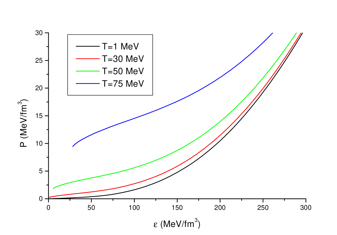
Figure 1: The equation of state for different temperature cases.

The thermodynamic properties of fermions can be evaluated using the well know functions $H_{n}$ and $G_{n}$ given by

$$H_{n}=\frac{1}{3\pi^{2}}\int_{0}^{\infty}\frac{k^{n-1}dk}{\sqrt{k^{2}+m_{F}^{2}}}\left\{f+\overline{f}\right\}$$ (25)

$$G_{n}=\frac{1}{\pi^{2}}\int_{0}^{\infty}k^{n-1}dk\left\{f-\overline{f}\right\}$$ (26)

The two terms in (25,26) correspond to the contributions of particles and antiparticles, respectively. Our first step is to calculate the pressure and energy density for nucleons which correspond to the nonrelativistic case. The relativistic case, corresponding to the high temperature approximation, is utilized in order to calculate the pressure coming from electrons and massive neutrinos. In this approach the function $H_{5}$ and $H_{3}$ are given by the following relations:

$$H_{3}(r,y)=\frac{1}{8}y^{2}(-1+2r^{2}+2\Gamma)+\frac{1}{4}y^{2}ln(y/\pi)$$ (27)

and

$$H_{5}(r,y)=-\frac{1}{32}r^{2}y^{2}+\frac{1}{96}(ry)^{4}-\frac{1}{64}y^{4}ln(y/\pi)+\frac{3}{256}-\frac{1}{64}\Gamma y^{4}.$$ (28)

In the case of massless neutrino ($m_{\nu}=0$) the pressure $P$ and the energy density $\varepsilon$ can be expressed analogously to the massive fermion relation (20). In this situation

$$P_{0\nu}=k_{B}^{4}T^{4}$$

and function $\phi$ is given by

$$\phi_{0}(z,t)=\frac{1}{3}\chi_{0}(z,t)=\frac{1}{3\pi^{2}}\int_{0}^{\infty}x^{3}dx\left\{\frac{1}{e^{(x-z)/t}+1}+\frac{1}{e^{(x+z)/t}+1}\right\}.$$ (29)

The function $\phi$ can be written with the use of the function $H_{n}$ defined as

$$H_{n}(r,y=0)=\int_{0}^{\infty}x^{n-2}dx\left\{\frac{1}{e^{(x-z)/t}+1}+\frac{1}{e^{(x+z)/t}+1}\right\}$$

In agreement with previous substitution the variable $r=z/t=\mu/k_{B}T$ and $z=\mu/M$. In this moment the case $y=0$ is considered. Having integrated these functions (29) one can obtain the results in which the solution is expressed by the polylogaritmic function $Li_{n}(z)$

$$\phi_{0}(z,t)=-\frac{6}{\pi^{2}}(Li_{4}(-e^{-z/t})+Li_{4}(-e^{z/t})).$$ (30)

In the case when the temperature ($T=0$) the integral $\phi_{i}$ and $\chi_{i}$ give as a solution the well-known Shapiro resalt [17]:

$$\phi(x)=\frac{1}{8\pi^{2}}\left\{x\sqrt{1+x^{2}}\left(\frac{2x^{2}}{3}-1\right)+\ln(x+\sqrt{1+x^{2}})\right\},$$

$$\chi(x)=\frac{1}{8\pi^{2}}\left\{x\sqrt{1+x^{2}}(1+2x^{2})-\ln(x+\sqrt{1+x^{2}})\right\}.$$

The total $\phi$ function is sum of the partial components

$$\phi=\phi_{n}+\phi_{p}+\phi_{e}+\phi_{\nu}.$$

The protoneutron star can be characterized by two parameters, the lepton fraction $Y_{L}$ and the entropy per nucleon $S$. The fermion number density and the entropy per nucleon are giving by the relations

$$n_{i}=\frac{1}{\pi^{2}}\int_{0}^{\infty}x^{2}dx\left\{f_{i}(x,z,t)-\overline{f}_{i}(x,z,t)\right\},$$ (31)

$$S\equiv\frac{s}{n_{B}}$$

while the fermions entropy density $s$ is defined as

$$s=\sum_{i}\frac{1}{\pi^{2}}\int_{0}^{\infty}dx\,x^{2}[-f_{i}(x,z,t)\ln f_{i}(x,z,t)-(1-f_{i}(x,z,t))\ln(1-f_{i}(x,z,t))$$

$$-\overline{f}_{i}(x,z,t)\ln\overline{f}_{i}(x,z,t)-(1-\overline{f}_{i}(x,z,t))\ln(1-\overline{f}_{i}(x,z,t))]$$

[18] with the use of the previously defined Dirac distribution functions $f_{i}$ and $\overline{f}_{i}$. Considering the case of massless neutrinos the equation (31) can be solved analytically and the final form of the neutrino number density is giving by

$$n_{0}=\frac{x^{2}t}{2\pi^{2}}\ln((1+e^{(x+\mu)/t})/(1+e^{(x-\mu)/t}))+$$

$$\frac{x\,t}{\pi^{2}}\sum_{p=(-,+)}Li_{2}(-e^{(x+p\mu)/t})+\frac{t^{2}}{\pi^{2}}\sum_{p=(-,+)}Li_{3}(-e^{(x+p\mu)/t})$$

The obtained result allows us to determine the lepton fraction $Y_{L}$, defined as

$$Y_{L}=\frac{n_{e}+n_{\nu}}{n_{B}}\,\,,$$ (32)

where $n_{B}$, $n_{e}$ and $n_{\nu}$ are the nucleon, electron and neutrino number densities, respectively. The proton fraction can be defined as

$$Y_{P}=\frac{n_{p}}{n_{B}},$$ (33)

where $n_{p}$ is proton number density. The difference between an ordinary neutron star and a protoneutron star is caused mainly by the high lepton number of the protoneutron star matter. This is because a star core is opaque to neutrinos. The lepton number is approximately constant after core bounce $Y_{L}$ $\simeq$ $0.4$ for the densities above $10^{12}$ $g/cm^{3}$ [1] - $10^{13}$ $g/cm^{3}$ [4] where the neutrinos are trapped. At the time the entropy per baryon is approximately constant $S\sim 1$. Below this density the neutrinos are free and they can escape. After the leak out of neutrinos their chemical potential vanishes.

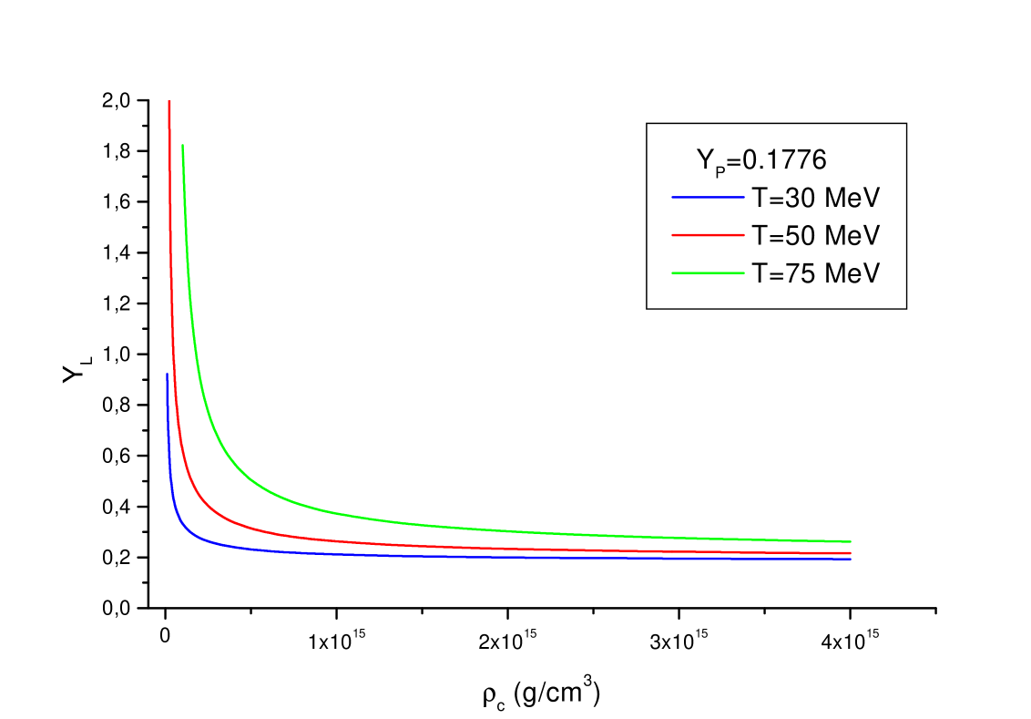
Figure 2: The lepton number $Y_{L}$ dependence on the central density $\rho_{c}$ for the different temperatures and for the constant proton fraction $Y_{P}=0.1776$.

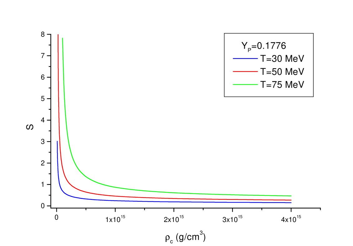
Figure 3: The entropy $S$ dependence on the central density $\rho_{c}$ for the different temperatures and $Y_{P}=0.1776$.

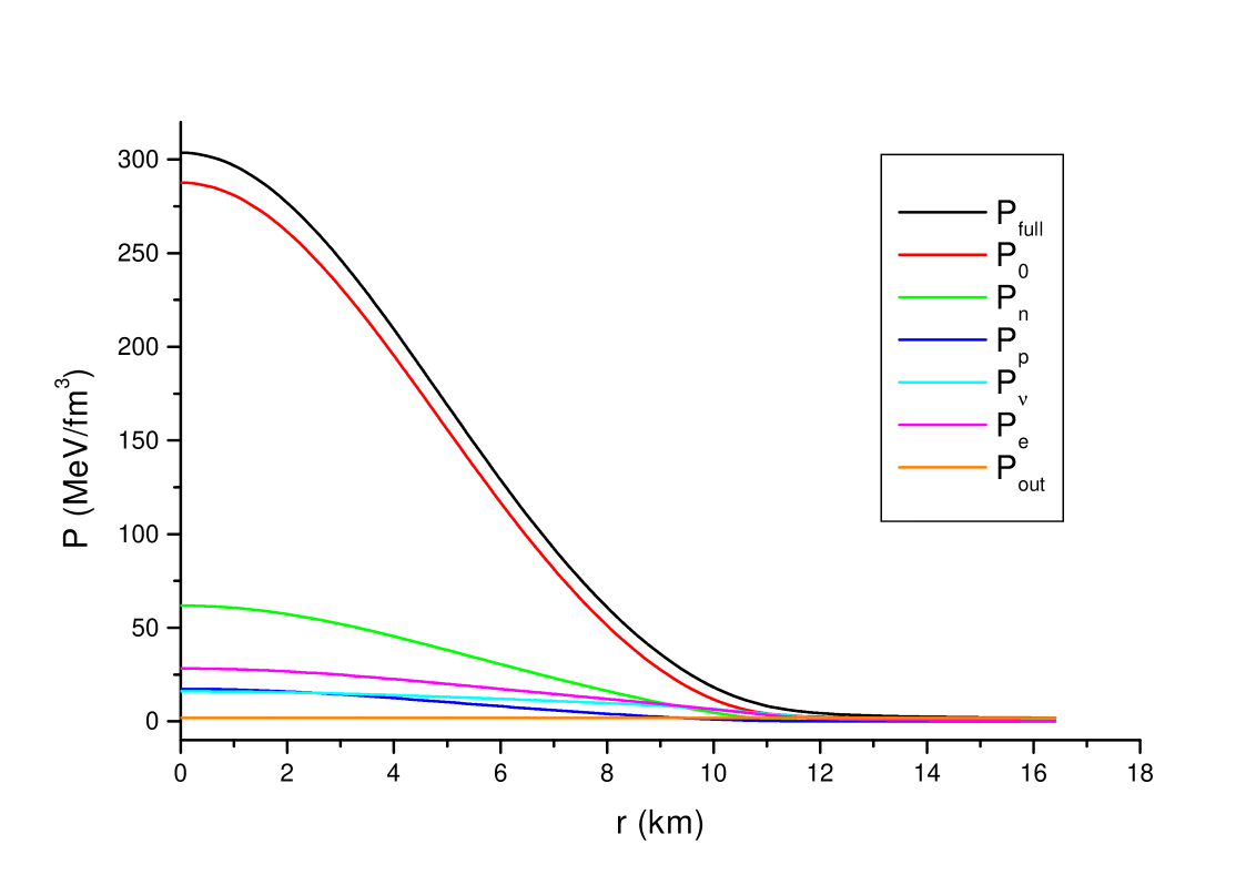
Figure 4: The pressure $P$ versus the radius $r$ for different components of pressure. The temperature is fixed $T=50$ $MeV$, $\rho_{c}=1.8$ $10^{15}$ $g/cm^{3}$.

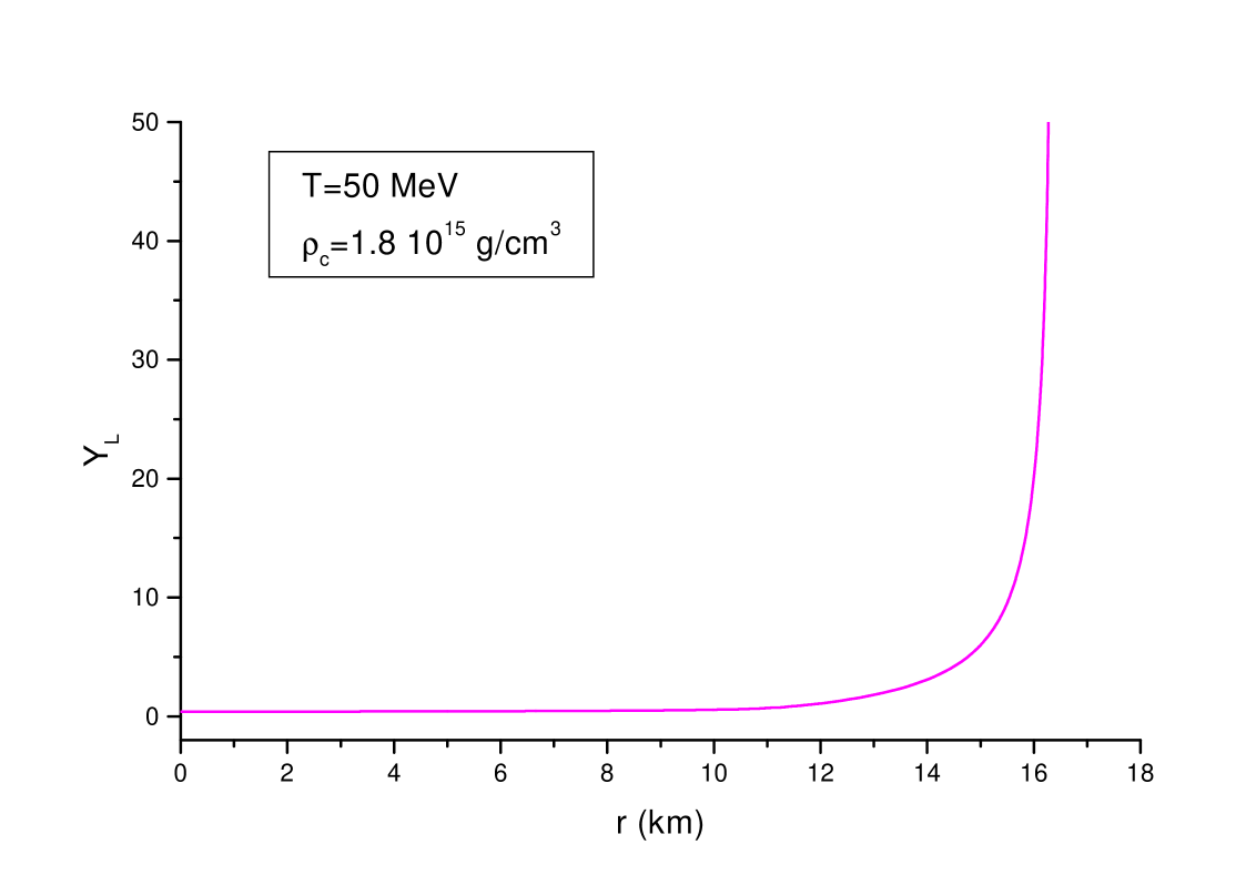
Figure 5: The lepton number $Y_{L}$ dependence on the radius $r$ for the temperature $T=50$ $MeV$ and $\rho_{c}=1.8$ $10^{15}g/cm^{3}$.

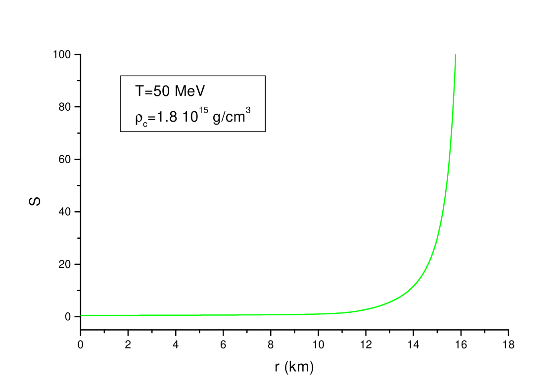
Figure 6: The entropy $S$ dependence on the radius $r$ for the temperature $T=50$ $MeV$ and $\rho_{c}=1.8$ $10^{15}g/cm^{3}$.

The situation, when the neutrinos are trapped, is characteristic to very initial stage of a protoneutron star existence. The matter is assumed to be composed of nucleons and leptons. Thus we are dealing here with electrically neutral matter being in $\beta$ equilibrium which can be expressed as a relation between the chemical potentials of the protoneutron star components.

$$\mu_{n}+\mu_{e}=\mu_{\nu_{e}}+\mu_{p}.$$ (34)

This equation can be written in terms of neutron $x_{n}$ and proton $x_{p}$ Fermi momentum

$$x_{p}=\left(\frac{Y_{P}}{1-Y_{P}}\right)^{\frac{1}{3}}x_{n}$$

$$\sqrt{\delta^{2}_{e}+x_{e}^{2}}+\sqrt{\delta^{2}_{p}+x_{p}^{2}}=\sqrt{\delta^{2}_{n}+x_{n}^{2}}+\sqrt{\delta^{2}_{\nu}+x_{\nu}^{2}}$$

for electrons and neutrinos $(i=e,\nu)$ $\delta_{i}=m_{e}/M,0$ whereas for nucleons $\delta=\delta_{n}=\delta_{p}$. Fermi momentum can be effectively only a function of the neutron Fermi momentum $x_{n}$ and the $Y_{P}$ parameter, which measures the proton admixture in the neutron star. The protoneutron star matter in general is more symmetric than neutron star matter.

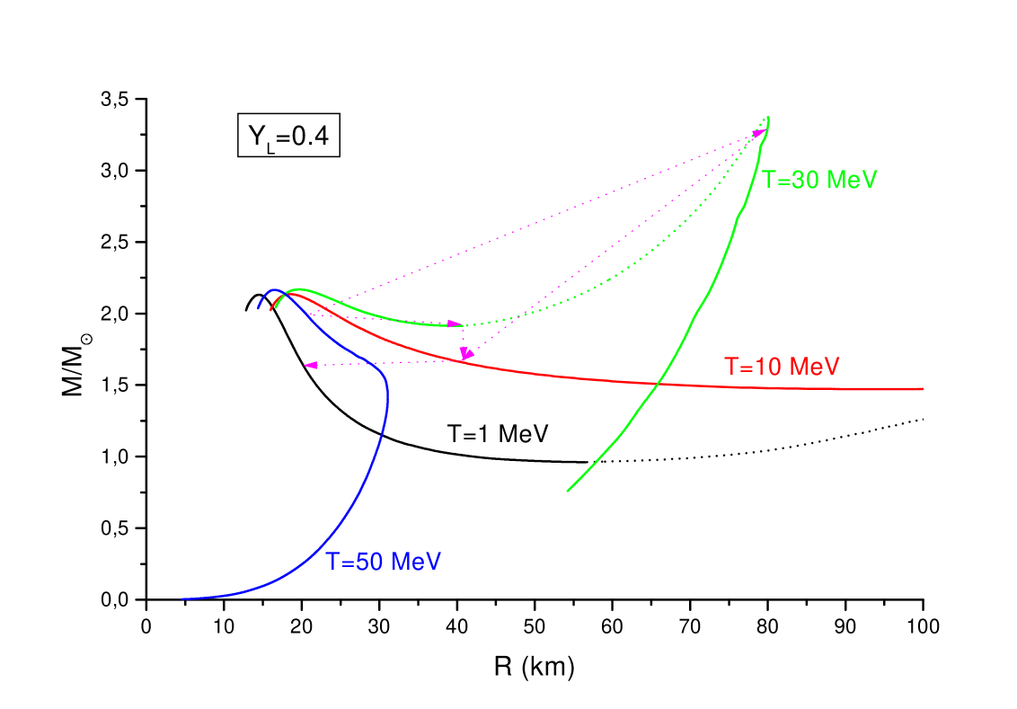
Figure 7: The mass-radius diagram for the protoneutron star for constant $Y_{L}=0.4$.

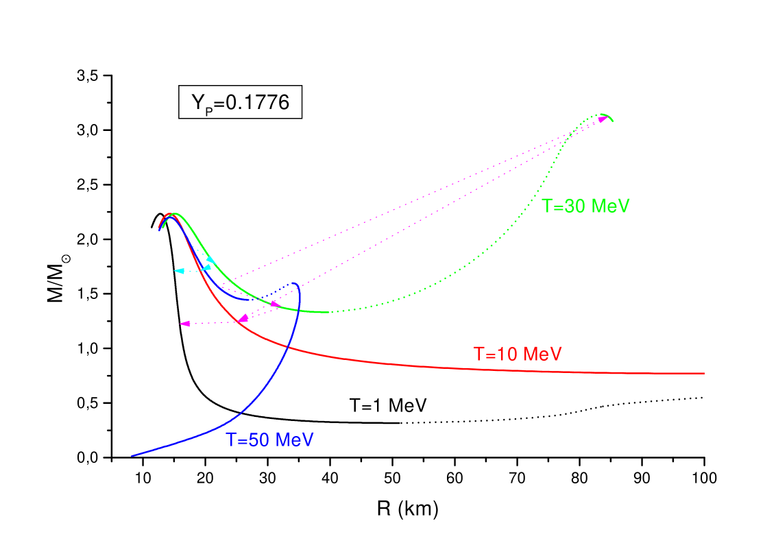
Figure 8: The mass-radius diagram for the protoneutron star for constant $Y_{P}=0.1776$.

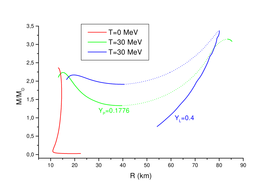
Figure 9: The mass-radius diagram for the protoneutron star with $T=30$ $MeV$ ($Y_{L}=0.4$, $Y_{P}=0.1776$) and $T=0$ $MeV$( the proton fraction is constrained by $\beta$ decay).

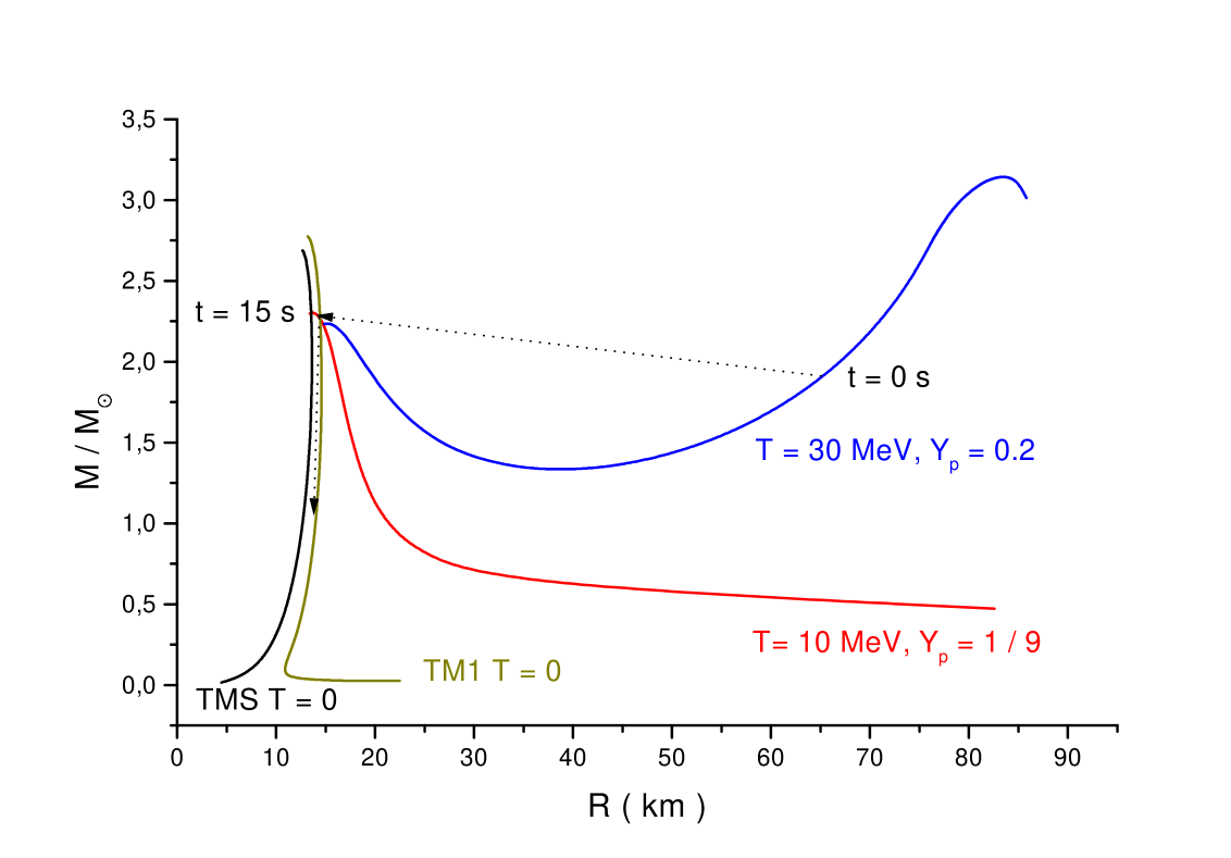
Figure 10: The time evolution ($t=0-15s$) of the protoneutron star (with $M{B}=1M_{\odot}$) in accordance with paper Toki [25].

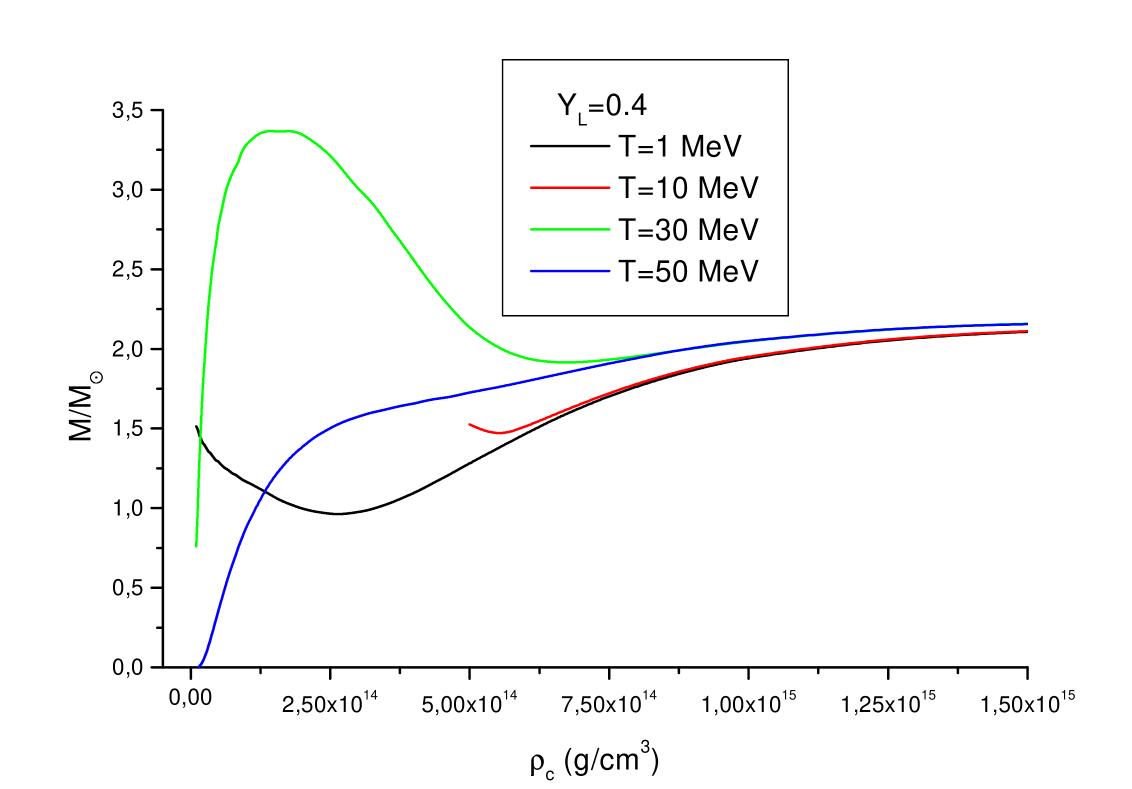
Figure 11: The mass $M$ dependence on the central density $\rho_{c}$ for $Y_{L}=0.4$.

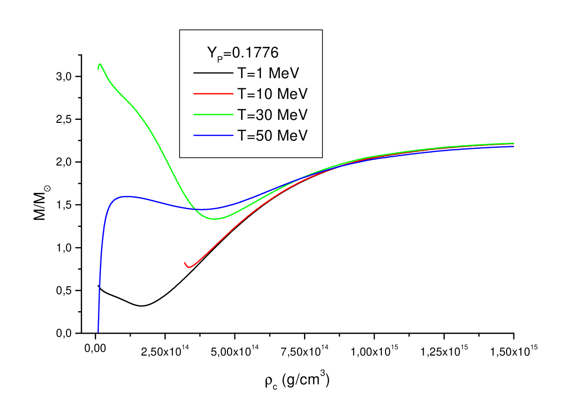
Figure 12: The mass $M$ dependence on the central density $\rho_{c}$ for $Y_{P}=0.1776$.

3 Rotating protoneutron star

The spacetime outside a rotating protoneutron star is much more complicated than the metric outside a non-rotating star thus it seems to be interesting to investigate the properties of rotating protoneutron stars. In general the metric of a stationary, axisymmetric, asymptotically flat spacetime has the form

$$ds^{2}=g_{\mu\nu}dx^{\mu}dx^{\nu}=-e^{2{\nu}}c^{2}dt^{2}+e^{2{\psi}}(d{\phi}-{\omega}cdt)^{2}+e^{2{\mu}}d{\theta}^{2}+e^{2{\lambda}}dr^{2},$$ (35)

with $g_{\mu\nu}$ being the metric tensor. The metric potential functions $\nu,\psi,\mu$ and $\lambda$ and the angular velocity $\omega$ of the stellar fluid in the local inertial frame are functions of the radial coordinate $r$ and the polar angel $\theta$ [22, 23]. In order to compute the structure of rapidly rotating fluid body the numerical method developed by Butterworth and Ipser [24] was introduced. Besides this exact numerical treatment there is a perturbative Hartle’s method which is based on the assumption that rotating massive body is no longer spherically symmetric. It is destorted, thus expanding the metric functions through second order in the stars rotational velocity $\Omega$ one can obtain the following form of the perturbed metric

$$ds^{2}=g_{\mu\nu}dx^{\mu}dx^{\nu}=-e^{2{\nu}(r,\;{\theta},\;{\Omega})}c^{2}dt^{2}+e^{2{\psi}(r,\;{\theta},\;{\Omega})}(d{\phi}-{\omega}(r,\;{\theta},\;{\Omega})cdt)^{2}$$

$$+e^{2{\mu}(r,\;{\theta},\;{\Omega})}d{\theta}^{2}+e^{2{\lambda}(r,\;{\theta},\;{\Omega})}dr^{2}+O(\Omega^{3}),$$

where metric functions in this perturbed line element are given by

$$e^{2{\nu}(r,\;{\theta},\;{\Omega})}=e^{2{\Phi}(r)}(1+2(h_{0}(r,{\Omega})+h_{2}(r,\;{\Omega})P_{2}(cos{\theta}))),$$

$$e^{2{\psi}(r,\;{\theta},\;{\Omega})}=r^{2}sin^{2}{\theta}(1+2(v_{2}(r,\;{\Omega})-h_{2}(r,\;{\Omega}))P_{2}(cos{\theta})),$$

$$e^{2{\mu}(r,\;{\theta},\;{\Omega})}=r^{2}(1+2(v_{2}(r,\;{\Omega})-h_{2}(r,\;{\Omega}))P_{2}(cos{\theta})),$$

$$e^{2{\lambda}(r,\;{\theta},\;{\Omega})}=e^{2{\Lambda}(r)}\left(1+\frac{2G}{c^{2}r}\frac{m_{0}(r,\;{\Omega})+m_{2}(r,\;{\Omega})P_{2}(cos{\theta})}{(1-\frac{2G}{c^{2}}\frac{m(r)}{r})}\right),$$ (36)

where $\Phi(r)$ and $\Lambda(r)$ are the metric functions of a spherically symmetric star, $P_{2}$ the Legendre polynomial of order 2, $m_{0},m_{2},h_{0},h_{2}$ and $\upsilon_{2}$ are all functions of $r$ and $\Omega$ [19, 6]. They are calculated from Einstein’s field equations and given as solutions of Hartle’s stellar structure equations, $\omega$ has the same meaning as in the nonperturbative line element (35). The metric functions are determined with the use of the Einstein equations

$$G_{\mu\nu}\equiv R_{\mu\nu}-\frac{1}{2}g_{\mu\nu}R={\kappa}T_{\mu\nu},$$ (37)

where $T_{\mu\nu}$ is the stress-energy tensor given in the perfect fluid form

$$T_{\mu\nu}=(\epsilon+P)u_{\mu}u_{\nu}+g_{\mu\nu}P$$ (38)

and $u_{\mu}$ is the unite four-velocity satisfying the following condition

$$u_{\mu}u^{\mu}=-I.$$

where $\epsilon$ is the total energy density, $P$ the pressure. Each metric function, namely $\nu,\rho$ and $\omega$ are functions of the radial coordinate $r$, polar angle $\theta$ and also the stars angular velocity $\Omega$. In the case of rotating stars there is an additional dependence of the metric on the polar angle and the frame dragging frequency $\omega$. The latter leads to the existence of the non-diagonal term $g^{t\varphi}$ in the metric tensor. The assumption of uniform rotation means that the value of $\Omega$ is constant throughout the star. For uniformly rotating bodies there is a relation between components of the four-velocity vector $u^{\varphi}=\Omega u^{t}$. The nonzero components of the four-velocity vector $u_{\mu}$ of the matter are of the form

$$u^{t}=(e^{2\nu(r,\theta)}-\overline{\omega}^{2}e^{2\psi(r,\theta)})^{-\frac{1}{2}},\hskip 28.45274ptu^{\varphi}=\Omega u^{t}$$ (39)

where

$$\overline{\omega}=\Omega-\omega\hskip 28.45274pt\Omega=\frac{d\varphi}{dt}$$ (40)

The absolute limit on stable neutron star rotation is the Kepler frequency $\Omega_{K}$. It determines the frequency at which the mass shedding at the stellar equator sets in. The result of the work of Haensel and Zdunik [26] shows that the value of the Kepler frequency can be estimated knowing the value of the mass and radius of the corresponding nonrotating star and an empirical relation was given

$$\Omega_{K}\approx C_{Hz}\sqrt{(M_{s}/M_{\odot})(R_{s}/10km)^{3}}=(0.63-0.67)\times\Omega_{c}$$ (41)

where, $C_{Hz}=7700s^{-1}$ and $\Omega_{c}$ is the Newtonian value and is equal

$$\Omega_{c}=\sqrt{M_{s}/R_{s}^{3}}$$ (42)

the index $s$ indicates that these values refer to the spherical configuration. As a consequence of the perturbative method for the angular velocity of the local inertial frame appears

$$\frac{d}{dr}\left(r^{4}j(r)\frac{d\overline{\omega}(r)}{dr}\right)+4r^{3}\frac{dj(r)}{dr}\overline{\omega}(r)=0,$$ (43)

where $\overline{\omega}={\Omega}-{\omega}$ and $j(r)=e^{-{\Phi}(r)}(1-\frac{2G}{c^{2}}\frac{m(r)}{r})^{\frac{1}{2}}$ and the boundary conditions are such that $\overline{\omega}(0)=\overline{\omega}_{c}$ and $\left(\frac{d\overline{\omega}}{dr}\right)_{r=0}=0$. The angular velocity dependence on the angular velocity in the center is stated as

$${\Omega}({\omega}_{c})=\overline{\omega}(R_{s})-\frac{R_{s}}{3}\left(\frac{d\overline{\omega}(r)}{dr}\right)_{r=R_{s}}.$$ (44)

The solution of equation $(\ref{om_{0}})$ allows us to determine the star’s momentum of inertia

$$I=\frac{J({\Omega})}{{\Omega}}=\frac{8{\pi}}{3c^{2}}\int_{0}^{R_{s}}drr^{4}\frac{{\varepsilon}(r)+P(r)}{(1-\frac{2G}{c^{2}}\frac{m(r)}{r})^{\frac{1}{2}}}\frac{\overline{\omega}(r)}{{\Omega}}e^{-{\Phi}(r)}.$$ (45)

The $\Omega_{c}$ is angular velocity in the approximation the amount needed to produce shedding of mass at the star’s equator, so that this method of computation is not actually valid for this large a value of $\Omega$.

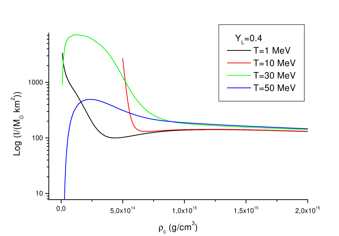
Figure 13: The moment of inertia $I$, (in units of $M_{\odot}$ $km^{2}$) as a function of the central density for the different temperatures. The lepton number equals 0.4.

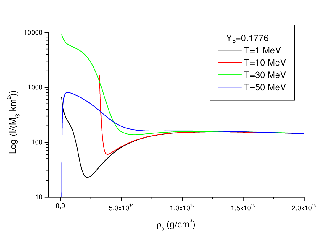
Figure 14: The moment of inertia $I$, (in units of $M_{\odot}$ $km^{2}$) as a function of the central density for the different temperatures. The proton number equals 0.1776.

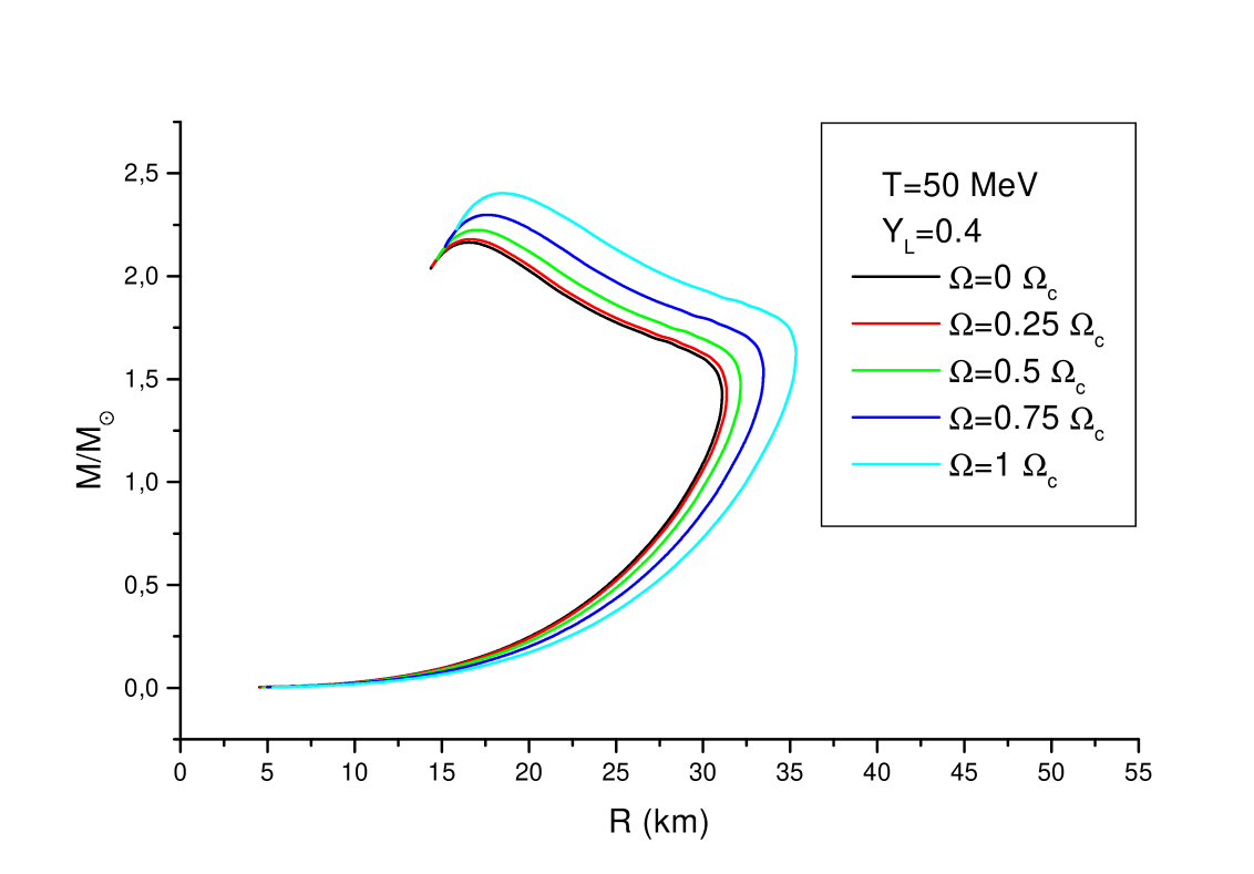
Figure 15: The mass-radius relation for the protoneutron star for different value of $\Omega$. The temperature $T$ and the lepton number $Y_{L}$ are fixed and equal $50$ $MeV$ and $0.4$, respectively.

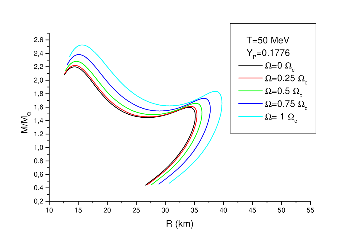
Figure 16: The mass-radius relation for the protoneutron star for different value of $\Omega$. The temperature $T$ and the proton fraction $Y_{P}$ are fixed and equal $50$ $MeV$ and $0.1776$, respectively.

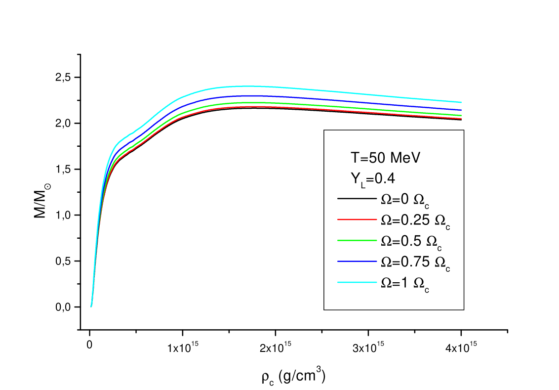
Figure 17: The mass-central density relation for the protoneutron star for different value of $\Omega$. The temperature $T$ and the lepton number $Y_{L}$ are fixed and equal $50$ $MeV$ and $0.4$, respectively.

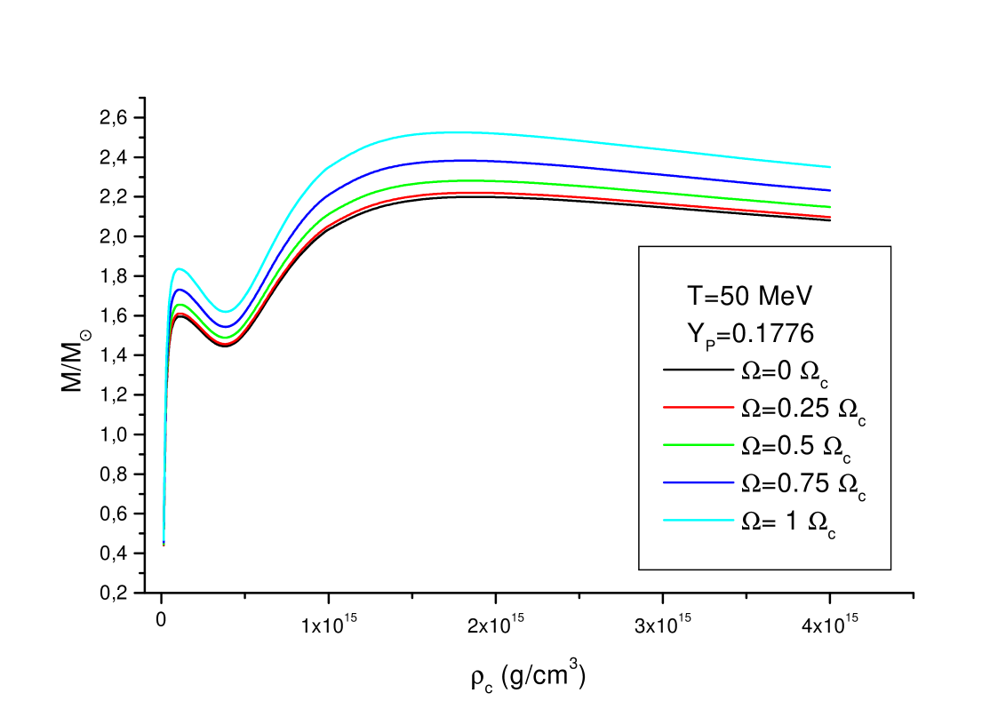
Figure 18: The mass-central density relation for the protoneutron star for different value of $\Omega$. The temperature $T$ and the proton fraction $Y_{P}$ are fixed and equal $50$ $MeV$ and $0.1776$, respectively.

4 The numerical results.

In this paper the behaviour of a protoneutron star in the RMF approach was examined. In Fig.1 the pressure P as a function of the energy density is shown for the TM1 parameter set in the case of finite temperature. The relevant temperature range is between 1 MeV up to 75 MeV. Figures 2 and 3 display the lepton fraction $Y_{L}=(n_{e}+n_{\nu})/n_{B}$ and the entropy as a function of central energy density. For different temperatures the proton fraction $Y_{P}$ is fixed and equal $Y_{P}=0.1776$. The pressure as the function of the star radius is presented in Fig.4. The total pressure of the protoneutron star being the sum of fermion and meson parts is denoted by $P_{full}$. Particular contributions $P_{\nu}$, $P_{p}$, $P_{n}$, $P_{e}$, $P_{out}$, $P_{o}$ mark the pressure coming from neutrinos, protons, neutrons, electrons, thermal plasma and pressure without neutrinos, respectively. Neutrons pressure is the most significant component of the total pressure whereas contributions coming from neutrinos and protons are nearly the same in the star core. As the radius increases the neutrino pressure starts to prevail over the remaining pressures. Figs.5 and 6 depict the lepton number $Y_{L}$ and the entropy per baryon $s$ as the function of the radius. The temperature is fixed and equals $50$ MeV, $\rho_{c}=1.8\times 10^{15}$ $g/cm^{3}$. For the considerable value of the star radius the lepton number and the entropy are almost constant whereas in the outer layers of the protoneutron star both of them grow very steeply. The mass-radius relations for protoneutron stars for different temperature cases and constant lepton $Y_{L}$ and proton $Y_{P}$ number is presented in the next two figures. The stable and unstable areas of the stellar configuration (the dotted line) are presented. The possible stellar evolution tracks with the constant baryon number are pointed by arrows. Considering configurations obtained for different temperatures one can see the possible evolution tracks. They are presented in Table 2 and Table 3.

$T\,[\,MeV\,]$	$R\,[\,km\,]$	$M\,[\,M_{\odot}\,]$
$50$	$20.8981$	$1.9751$
$30$	$79.9505$	$3.2871$
	$40.6529$	$1.9139$
$10$	$40.5229$	$1.6566$
$1$	$20.2331$	$1.6328$

Table 2: The evolution tracks for $Y_{L}=0.4$.

$T\,[\,MeV\,]$	$R\,[\,km\,]$	$M\,[\,M_{\odot}\,]$
$50$	$22.1870$	$1.5560$
$30$	$84.6644$	$3.1236$
	$32.2714$	$1.3731$
$10$	$25.2496$	$1.2360$
$1$	$15.8983$	$1.2232$

Table 3: The evolution tracks for $Y_{P}=0.1776$.

At the initial time $t=0$ s the protoneutron star is characterized by the barion mass of the value of 1 $M_{\odot}$ and the proton fraction $Y_{P}=0.2$, the temperature equals 30 MeV. In accordance with the radial profiles of temperature present in paper [25] after 15 s the temperature and the proton fraction drop to 10 MeV and $1/9$, respectively. For comparison the mass-radius dependence for the protoneutron star with constant lepton and proton number and in the temperature equal $30$ MeV are presented in Fig.9. The unstable configurations appear and they are marked by dotted lines. The same relation is shown for the star in zero temperature limit and with zero neutrino chemical potential (without neutrinos), than the proton concentration is constrained by the $\beta$ equilibrium. The mass-central density ($\rho_{c}$) functions for different temperatures and fixed lepton number $Y_{L}$ (Fig.11) and proton fraction $Y_{P}$ (Fig.12) are shown on Figs.11 and 12. From relations presented on Figs.7 and 8 one can see the density ranges for which the stars are stable. Using the results of Figs.7 and 8 the density ranges of unstable protoneutron stars configurations can be estimated. The moment of inertia ($I$) of a protoneutron star versus the central density ($\rho_{c}$) for different values of temperature are presented. Figures 15 and 16 show the subsequence mass-radius relations of a hot protoneutron star ($T=50$ $MeV$) obtained for different angular velocities. The lepton and proton number are constant. The greatest values of the angular velocity the more massive and bigger are the stars. Figures 17 and 18 compare the mass-central density relations for protoneutron stars with fixed values of lepton $Y_{L}$ and proton $Y_{P}$ number. The temperature equals $50$ $MeV$ obtained for different angular velocities. In Fig.18 the density range of stable rotating protoneutron star is visable. The main numerical results is collected in the Table 4 and the Table 5, where $Y_{L}=0.4$ and $\rho_{c}=5$ $10^{14}$ $g/cm^{3}$.

$T\,[\,MeV\,]$	$R\,[\,km\,]$	$M\,[\,M_{\odot}\,]$	$M_{B}\,[\,M_{\odot}\,]$	$I\,[\,M_{\odot}\,km^{2}]$
$1$	$14.3886$	$2.1312$	$2.3057$	$130.4967$
$10$	$18.3521$	$2.135$	$2.3051$	$131.3594$
$30$	$80.0136$	$3.3723$	$1.7768$	$123.7578$
	$19.6225$	$2.1694$	$2.2806$	$146.7724$
$50$	$16.4648$	$2.1659$	$2.1226$	$152.4982$
$75$	$12.5894$	$1.9839$	$1.7173$	$116.9361$

Table 4: The mass, the radius and the moment of inertia for $Y_{L}=0.4$.

$T\,[\,MeV\,]$	$R\,[\,km\,]$	$\overline{R}\,[\,km\,]$	$M\,[\,M_{\odot}\,]$	$\overline{M}\,[\,M_{\odot}\,]$	$J\,[\,M_{\odot}\,km^{2}\,s^{-1}\,]$
$1$	$14.3886$	$15.6158$	$2.1312$	$2.4281$	$1271590$
$10$	$18.3521$	$20.9522$	$2.135$	$2.2798$	$889378$
$30$	$80.0136$	$92.0202$	$3.3722$	$3.7851$	$6658570$
	$19.6225$	$22.5576$	$2.1694$	$2.3129$	$906022$
$50$	$16.4648$	$18.2002$	$2.1659$	$2.4031$	$1223790$
$75$	$12.5894$	$13.4091$	$1.9839$	$2.3060$	$1343250$

Table 5: The mass, the radius and the angular momentum for $Y_{L}=0.4$.

5 The conclusion.

The main aim of this paper was to study the protoneutron star parameters especially the masses and radii as the most sensitive ones to the form the equation of state. The employed form of EOS in the TM1 set which was extended to the finite temperature cases. The considered model comprises not only nucleons and electrons, which are necessary for the $\beta$ stable matter, but the neutrinos as well. The presence of neutrinos is characteristic for hot young protoneutron stars. Neutrinos give not negligible contribution to the pressure and energy density. As the radius of protoneutron stars increases the neutrino pressure starts to prevail over the pressure coming from the remaining components. Constructing the mass-radius relations for protoneutron stars the stable and unstable areas appeared. This indicate that there are several possible stellar evolution tracks for the configuration with constant baryon number. These evolutionary tracks are strictly connected with the decreasing star temperature and thus with the decreasing neutrino chemical potential and lepton number. The final result is the cold deleptonized (the neutrino chemical potential equals zero) object. The influence of rotation on the protoneutron star parameters is significant. In this paper the case of slowly rotating protoneutron star is considered. The obtained unstable configuration for the fixed temperature ($T=30$ MeV) and lepton number ($Y_{L}=0.4$) occurring in the density range ($1.4-6.5\times 10^{14}$ $g/cm^{3}$) are relevant to rapid change in the moment of inertia of the star (Fig.13 and Fig.14). For the rotating star the mass-radius relation depends on the star angular velocity thus the values of $\Omega$ affects the instability areas. For the employed EOS there exists the ranges of masses where hot, lepton rich protoneutron star can be stabilized against gravity but loosing leptons these objects became gravitationally unstable. The instability areas as strictly connected with the presence of neutrinos and the thermal pressure effects.

References

References

• [1] Strobel K, Schaab C and Weigel M K Properties of non-rotating and rapidly rotating protoneutron stars Preprint astro-ph/9908132
• [2] Dutta R, The role of trapped neutrino in dense stellar matter and kaon condensation Preprint nucl-th/9812058
• [3] Reddy S, Bertsch G and Prakash M First order phase transition in neutron star matter: droplets and coherent neutrino scattering Preprint nucl-th/9909040
• [4] Prakash M 1994 The equation of state and neutron stars
• [5] Reddy S, Pons J, Prakash M and Lattimer J M Neutrino opacities at high density and the protoneutron star evolution, Preprint astro-ph/9802312
• [6] Weber F 1999 Pulsars as astrophysical laboratories for nuclear and particle physics IOP Publishing
• [7] Reinhard P G, Rufa M, Maruhn J, Greiner W and Friedrich J 1986 Atomic nuclei Z. Phys. A 323 13-25
• [8] Serot B D and Walecka J D 1997 Recent progress in quantum hydrodynamics Int. J. Mod. Phys. E6 515-631
• [9] Bednarek I and MaΕ„ka R. 2000 The hot neutron star Physica Scripta V61 544-549
• [10] Bednarek I, MaΕ„ka R and PrzybyΕ‚a G 2000 The neutron star in relativistic mean-field theory Phys. Rev. C62 015802
• [11] Prakash M, Ainsworth T L and Lattimer J M Equation of state and the maximum mass of neutron star Phys. Rev. Letters V61 22 2518
• [12] Reddy S, Prakash M and Lattimer J M Neutrino interactions in hot and dense matter Phys. Rev. D 58 013009
• [13] Pons J A, Reddy S, Prakash M, Lattimer J M and Miralles J A Evolution of protoneutron stars Preprint astro-ph/9807040
• [14] Glendenning N K 1997 Compact stars Sringer-Verlag
• [15] Boguta J and Bodmer A R 1977 Nucl. Phys. A292 413
• [16] Sughara Y and Toki H 1994 Prog. Theo. Phys. 92 803
• [17] Shapiro S L and Teukolsky S A 1983 Black hols, white dwarfs and neutron stars New York
• [18] Sumiyoshi K and Toki H 1994 Relativistic equation of state of nuclear matter for the supernova explosion and the birth of neutron stars ApJ 422 700-718
• [19] Hartle J B 1967 ApJ 150 1005
• [20] Hartle J B and Thorne K S 1968 ApJ 153 807
• [21] Butterworth E M and Ipser J R 1976 ApJ 204 200
• [22] Hartle J B 1967 ApJ 150 1005
• [23] Hartle J B and Thorne K S 1968 ApJ 153 807
• [24] Butterworth E M and Ipser J R 1976 ApJ 204 200
• [25] Sumiyoshi K, Suzuki H and Toki H 1977 Influence of the symmetry energy on the birth of neutron stars and supernova neutrinos Nucl. Phys. Preprint astro-ph/9506024
• [26] Haensel P and Zdunik J L 1989 Nature 340 617