Power Spectrum Covariance of Weak Gravitational Lensing

Abstract

Weak gravitational lensing observations probe the spectrum and evolution of density fluctuations and the cosmological parameters which govern them. At low redshifts, the non-linear gravitational evolution of large scale structure produces a non-Gaussian covariance in the shear power spectrum measurements that affects their translation into cosmological parameters. Using the dark matter halo approach, we study the covariance of binned band power spectrum estimates and the four point function of the dark matter density field that underlies it. We compare this semi-analytic estimate to results from N-body numerical simulations and find good agreement. We find that for a survey out to z $\sim$ 1, the power spectrum covariance increases the errors on cosmological parameters determined under the Gaussian assumption by about 15%.

1. Introduction

Weak gravitational lensing by large scale structure (LSS) shears the images of faint galaxies at the percent level and correlates their measured ellipticities (e.g., Blaetal91 1991; Mir91 1991; Kai92 1992). Though challenging to measure, the two point correlations, and the power spectrum that underlies them, provide important cosmological information that is complementary to that supplied by the cosmic microwave background and potentially as precise (e.g., JaiSel97 1997; Beretal97 1997; Kai98 1998; HuTeg99 1999; Hui99 1999; Coo99 1999; Vanetal99 1999; see BarSch00 2000 for a recent review). Indeed several recent studies have provided the first clear evidence for weak lensing in so-called blank fields where the large scale structure signal is expected to dominate (e.g., Vanetal00 2000; Bacetal00 2000; Witetal00 2000; Kaietal00 2000).

Given that weak gravitational lensing probes the projected mass distribution, its statistical properties reflect those of the dark matter. Non-linearities in the mass distribution, due to gravitational evolution at low redshifts, causes the shear field to become non-Gaussian. It is well known that lensing induces a measureable three-point correlation in the derived convergence field (Beretal97 1997; CooHu00 2000). The same processes also induce a four point correlation. The four point correlations are of particular interest in that they quantify the sample variance and covariance of two point correlation or power spectrum measurements. Previous studies of the ability of power spectrum measurements to constrain cosmology have been based on a Gaussian approximation to the sample variance and the assumption that covariance is negligible (e.g., HuTeg99 1999); it is of interest to test to what extent their inferences remain valid in the presence of realistic non-Gaussianity. More importantly, when interpreting the power spectrum recovered from the next generation of surveys an accurate propagation of errors will be critical (HuWhi00 2000).

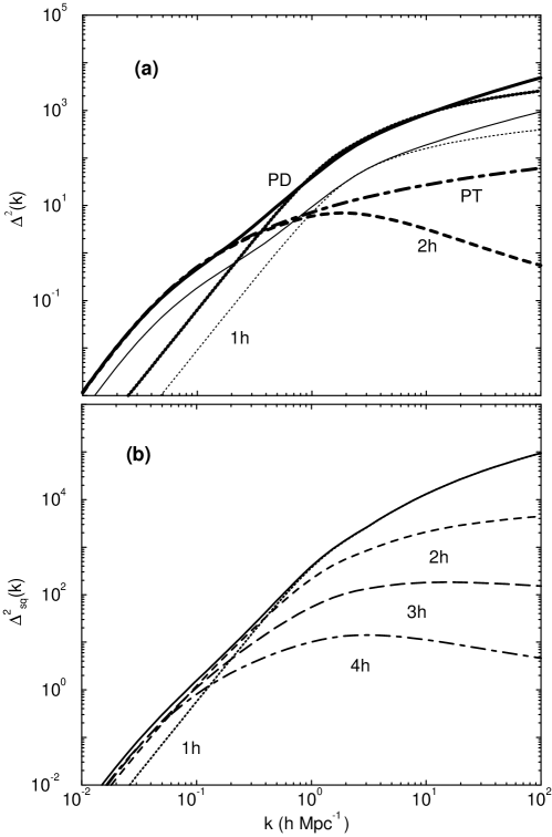
Figure 1.— The dark matter power spectrum (a) and square-configuration trispectrum (b) broken into individual contributions under the halo description. The lines labeled ’PD’ shows the dark matter power spectrum under the PeaDod96 (1996) non-linear fitting function while the curve labeled ’PT’ is the linear dark matter power spectrum (at redshift of 0). In (a), we show the power spectrum at redshifts of 0 and 1. In (b), we show the square configuration trispectrum (see text). In both (a) and (b), at small scales the single halo term dominates while at large scales halo correlations contribute.

Here, we present a semi-analytical estimate of the Fourier analogue of the four point function, i.e. the trispectrum, and calculate in detail the configurations that contribute to power spectrum covariance. Since weak lensing shear and convergence can be written as a simple projection of the dark matter density field, the problem reduces to a study of the trispectrum of the density field. Previous studies of the dark matter trispectrum have employed a mix of perturbation theory and non-linear scalings (e.g., Scoetal99 1999) or N-body simulations (MeiWhi99 1999). The former are not applicable to the full range of scales and configurations of interest; the latter are limited by computational expense to a handful of realizations of cosmological models with modest dynamical range.

Here, we use the dark-matter halo approach to model the density field (Sel00 2000; MaFry00a 2000a; Scoetal00 2000) and extend our previous treatments of the two-point and three-point lensing statistics (Cooetal00 2000; CooHu00 2000). The critical ingredients are: a mass function for the halo distribution, such as the Press-Schechter (PS; PreSch74 1974) mass function; a profile for the dark matter halo, e.g., the profile of Navetal96 (1996; NFW), and a description of halo biasing (Moetal97 1997). In the mildly non-linear regime, where most of the contribution to lensing is expected, the accuracy of the halo model has been extensively tested against simulations at the two point and three point levels (Sel00 2000; MaFry00a 2000a; Scoetal00 2000). We present tests here of the four point configurations involved in the power spectrum covariance. These techniques can also be extended to the covariance of the power spectrum of galaxy redshift surveys with a prescription for assigning galaxies to halos (Sel00 2000; Scoetal00 2000). The effect of non-Gaussianities on the measured galaxy power spectrum, through a measurement of the angular correlation function, is discussed in EisZal99 (1999).

In §2, we study the trispectrum of the dark matter density field under the halo model and test it against simulations from (MeiWhi99 1999). In §3, we apply these techniques to the the weak lensing covariance and test them against the simulations of (WhiHu99 1999). We also discuss the effect of power spectrum covariance on cosmological parameter estimation.

2. Dark Matter Power Spectrum Covariance

We begin by defining the power spectrum, trispectrum and power spectrum covariance in §2.1. We then derive the halo model for these quantities in §2.2. In §2.3, we present results and comparisons with $N$-body simulations.

2.1. General Definitions

The two and four point correlations of the density field are defined in the usual way

$$\left<\delta({\bf k}_{1})\delta({\bf k}_{2})\right> = (2\pi)^{3}\delta_{\rm D}({\bf k}_{12})P(k_{1})\,,$$ (1)

$$\left<\delta({\bf k}_{1})\ldots\delta({\bf k}_{4})\right>_{c} = (2\pi)^{3}\delta_{\rm D}({\bf k}_{1234})T({\bf k}_{1},{\bf k}_{2},{\bf k}_{3},{\bf k}_{4})\,,$$ (2)

where ${\bf k}_{i\ldots j}={\bf k}_{i}+\ldots+{\bf k}_{j}$ and $\delta_{\rm D}$ is the delta function not to be confused with the density perturbation. Note that the subscript $c$ denotes the connected piece, i.e. the trispectrum is defined to be identically zero for a Gaussian field. Here and throughout, we occasionally suppress the redshift dependence where no confusion will arise.

Because of the closure condition expressed by the delta function, the trispectrum may be viewed as a four-sided figure with sides ${\bf k}_{i}$. It can alternately be described by the length of the four sides $k_{i}$ plus the diagonals. We occasionally refer to elements of the trispectrum that differ by the length of the diagonals as different configurations of the trispectrum.

Following Scoetal99 (1999), we can relate the trispectrum to the variance of the estimator of the binned power spectrum

$$\hat{P}_{i}={1\over V}\int_{{\rm s}i}{d^{3}k\over V_{{\rm s}i}}\delta^{*}(-{\bf k})\delta({\bf k})\,,$$ (3)

where the integral is over a shell in $k$-space centered around $k_{i}$, $V_{{\rm s}i}\approx 4\pi k_{i}^{2}\delta k$ is the volume of the shell and $V$ is the volume of the survey. Recalling that $\delta({\bf 0})\rightarrow V/(2\pi)^{3}$ for a finite volume,

$$C_{ij} \equiv \left<\hat{P}_{i}\hat{P}_{j}\right>-\left<\hat{P}_{i}\right>\left<\hat{P}_{j}\right>$$ (4)

$$= {1\over V}\left[{(2\pi)^{3}\over V_{{\rm s}i}}2P_{i}^{2}\delta_{ij}+T_{ij}\right]\,,$$

where

$$T_{ij} \equiv \int_{{\rm s}i}{d^{3}k_{i}\over V_{{\rm s}i}}\int_{{\rm s}j}{d^{3}k_{j}\over V_{{\rm s}j}}T({\bf k}_{i},-{\bf k}_{i},{\bf k}_{j},-{\bf k}_{j})\,.$$ (5)

Notice that though both terms scale in the same way with the volume of the survey, only the Gaussian piece necessarily decreases with the volume of the shell. For the Gaussian piece, the sampling error reduces to a simple root-N mode counting of independent modes in a shell. The trispectrum quantifies the non-independence of the modes both within a shell and between shells. Calculating the covariance matrix of the power spectrum estimates reduces to averaging the elements of the trispectrum across configurations in the shell. It is to the subject of modeling the trispectrum that we now turn.

2.2. Halo Model

We model the power spectrum and trispectrum of the dark matter field under the halo approach. Here we present in detail the extensions required to model the trispectrum. We refer the reader to CooHu00 (2000) for a more in depth treatment of the ingredients.

The halo approach models the fully non-linear dark matter density field as a set of correlated discrete objects (“halos”) with profiles $\rho_{i}$ that for definiteness depend on their mass $M$ and concentration $c$ as in the NFW profile (Navetal96 1996)

$$\rho({\mathbf{x}})=\sum_{i}\rho_{\rm h}({\mathbf{x}}-{\mathbf{x}}_{i};M_{i},c_{i})\,,$$ (6)

and so a density fluctuation in Fourier space

$$\delta({\bf k}) = \sum_{i}e^{i{\bf k}\cdot{\mathbf{x}}_{i}}\delta_{{\rm h}}({\bf k};M;c)$$ (7)

$$= \sum_{V_{1},M_{1},c_{1}}n_{1}e^{i{\bf k}\cdot{\mathbf{x}}_{1}}\delta_{\rm h}({\bf k},M_{1},c_{1})\,,$$ (8)

where we have divided space up into volumes $\delta V$ sufficiently small such that they contain only one halo $n_{1}=n_{1}^{2}=n_{1}^{\mu}=$ $1$ or $0$ following Pee80 (1980). The final ingredient is that the halos themselves are taken to be biased tracers of the linear density field (denoted PT) such that their number density fluctuates as

$${d^{2}n\over dMdc}({\mathbf{x}})={d^{2}\bar{n}\over dMdc}[b_{0}+b_{1}(M)\delta_{\rm pt}({\mathbf{x}})+{1\over 2}b_{2}(M)\delta_{\rm pt}^{2}(\bf x)\ldots]$$ (9)

where $b_{0}\equiv 1$ and the halo bias parameters are given in Moetal97 (1997). Thus

$$\left<n_{1}\right> = {d^{2}\bar{n}\over dMdc}\delta M_{1}\delta c_{1}\,,$$ (10)

$$\left<n_{1}n_{2}\right> = \left<n_{1}\right>\delta_{12}+\left<n_{1}\right>\left<n_{2}\right>[b_{0}^{2}+b_{1}(M_{1})b_{1}(M_{2})\,,$$

$$\times\left<\delta_{\rm pt}({\mathbf{x}}_{1})\delta_{\rm pt}({\mathbf{x}}_{2})\right>]\,.$$

$$\left<n_{1}n_{2}n_{3}\right> = \ldots\,.$$ (11)

The derivation of the higher point functions in Fourier space is now a straightforward but tedious exercise in algebra. The Fourier transforms inherent in eqn. (8) convert the correlation functions in eqn. (11) into the power spectrum, bispectrum, trispectrum, etc., of perturbation theory.

Replacing sums with integrals, we obtain expressions based on the general integral

$$I_{\mu}^{\beta}(k_{1},\ldots,k_{\mu}) \equiv \int dM\int dc\frac{d^{2}\bar{n}}{dMdc}b_{\beta}(M)$$ (12)

$$\quad\delta_{\rm h}(k_{1},M,c)\ldots\delta_{\rm h}(k_{\mu},M,c)\,.$$

The index $\mu$ represents the number of points taken to be in the same halo such that $\left<n_{1}^{\mu}\right>=\left<n_{1}\right>$.

The power spectrum under the halo model becomes (Sel00 2000)

$$P(k) = P^{1h}(k)+P^{2h}(k)\,,$$ (13)

$$P^{1h}(k) = I_{2}^{0}(k,k)\,,$$ (14)

$$P^{2h}(k) = \left[I_{1}^{1}(k)\right]^{2}P^{\rm pt}(k)\,,$$ (15)

where the two terms represent contributions from two points in a single halo (1h) and points in different halos (2h) respectively.

Likewise for the trispectrum, the contributions may be separated into those involving one to four halos

$$T=T^{1h}+T^{2h}+T^{3h}+T^{4h}\,,$$ (16)

where here and below the argument of the trispectrum is understood to be $({\bf k}_{1},{\bf k}_{2},{\bf k}_{3},{\bf k}_{4})$. The term involving a single halo probes correlations of dark matter within that halo

$$T^{1h}=I_{4}^{0}(k_{1},k_{2},k_{3},k_{4})\,,$$ (17)

and is independent of configuration due to the assumed spherical symmetry for our halos.

The term involving two halos can be further broken up into two parts

$$T^{2h}=T^{2h}_{31}+T^{2h}_{22}\,,$$ (18)

which represent taking three or two points in the first halo

$$T^{2h}_{31}=P^{\rm pt}(k_{1})I_{3}^{1}(k_{2},k_{3},k_{4})I_{1}^{1}(k_{1})+3\;{\rm Perm.,}$$ (19)

$$T^{2h}_{22}=P^{\rm pt}(k_{12})I_{2}^{1}(k_{1},k_{2})I_{2}^{1}(k_{3},k_{4})+2\;{\rm Perm.}$$ (20)

The permutations involve the 3 other choices of $k_{i}$ for the $I_{1}^{1}$ term in the first equation and the two other pairings of the $k_{i}$’s for the $I_{2}^{1}$ terms in the second. Here, we have defined ${\bf k}_{12}={\bf k}_{1}+{\bf k}_{2}$; note that $k_{12}$ is the length of one of the diagonals in the configuration.

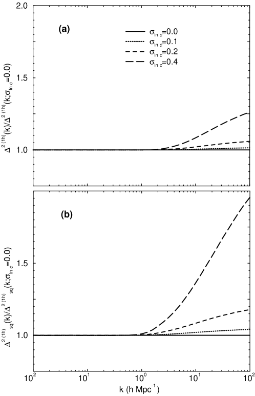
Figure 2.— The ratio of the single halo term contribution to that for a concentration width $\sigma_{\ln c}\rightarrow 0$ for the (a) power spectrum and (b) trispectrum. The small scale behavior is increasingly sensitive to the high concentration tails for the higher order statistics.

The term containing three halos can only arise with two points in one halo and one in each of the others

$$T^{3h} = B^{\rm pt}({\bf k}_{1},{\bf k}_{2},{\bf k}_{34})I_{2}^{1}(k_{3},k_{4})I_{1}^{1}(k_{1})I_{1}^{1}(k_{2})$$

$$+P^{\rm pt}(k_{1})P^{\rm pt}(k_{2})I_{2}^{2}(k_{3},k_{4})I_{1}^{1}(k_{1})I_{1}^{1}(k_{2})+5\;{\rm Perm.}\,,$$

where the permutations represent the unique pairings of the $k_{i}$’s in the $I_{2}$ factors. This term also depends on the configuration. The bispectrum in perturbation theory is given by

$$B^{\rm pt}({\bf k}_{p},{\bf k}_{q},{\bf k}_{r}) = 2F_{2}^{\rm s}({\bf k}_{p},{\bf k}_{q})P(k_{p})P(k_{q})+2\;{\rm Perm.}\,,$$ (22)

with $F_{2}^{\rm s}$ term given by second order gravitational perturbation calculations (see, below).

Finally for four halos, the contribution is

$$T^{4h} = I_{1}^{1}(k_{1})I_{1}^{1}(k_{2})I_{1}^{1}(k_{3})I_{1}^{1}(k_{4})\Big{\{}T^{\rm pt}+\Big{[}{I_{2}^{1}(k_{4})\over I_{1}^{1}(k_{4})}$$ (23)

$$\quad\times P^{\rm pt}(k_{1})P^{\rm pt}(k_{2})P^{\rm pt}(k_{3})+3\;{\rm Perm.}\Big{]}\Big{\}},$$

where the permutations represent the choice of $k_{i}$ in the $I^{1}$’s in the brackets. The perturbation trispectrum can be written as (Fry84 1984)

$$T^{\rm pt}=$$

$$\quad 4\left[F_{2}^{\rm s}({\bf k}_{12},-{\bf k}_{1})F_{2}^{\rm s}({\bf k}_{12},{\bf k}_{3})P(k_{1})P(k_{12})P(k_{3})+{\rm Perm.}\right]$$

$$\quad+6\left[F_{3}^{\rm s}({\bf k}_{1},{\bf k}_{2},{\bf k}_{3})P(k_{1})P(k_{2})P(k_{3})+{\rm Perm.}\right]\,.$$ (24)

The permutations involve a total of 12 terms in the first set and 4 terms in the second set. We now discuss the results from this modeling for a specific choice of halo input parameters and cosmology.

Table 1

Dark Matter Power Spectrum Correlations
$k$ 0.031 0.044 0.058 0.074 0.093 0.110 0.138 0.169 0.206 0.254 0.313 0.385 0.031 1.000 0.019 0.041 0.065 0.086 0.113 0.149 0.172 0.186 0.186 0.172 0.155 0.044 (-0.017) 1.000 0.036 0.075 0.111 0.153 0.204 0.238 0.261 0.264 0.251 0.230 0.058 (0.023) (0.001) 1.000 0.062 0.118 0.183 0.255 0.302 0.334 0.341 0.328 0.305 0.074 (0.024) (0.024) (0.041) 1.000 0.102 0.189 0.299 0.368 0.412 0.425 0.412 0.389 0.093 (0.042) (0.056) (0.027) (0.079) 1.000 0.160 0.295 0.404 0.466 0.485 0.475 0.453 0.110 (0.154) (0.076) (0.086) (0.094) (0.028) 1.000 0.277 0.433 0.541 0.576 0.570 0.549 0.138 (0.176) (0.118) (0.149) (0.202) (0.085) (0.205) 1.000 0.434 0.580 0.693 0.698 0.680 0.169 (0.188) (0.180) (0.138) (0.229) (0.177) (0.251) (0.281) 1.000 0.592 0.737 0.778 0.766 0.206 (0.224) (0.165) (0.177) (0.322) (0.193) (0.314) (0.396) (0.484) 1.000 0.748 0.839 0.848 0.254 (0.264) (0.228) (0.206) (0.343) (0.261) (0.355) (0.488) (0.606) (0.654) 1.000 0.858 0.896 0.313 (0.265) (0.234) (0.202) (0.374) (0.259) (0.397) (0.506) (0.618) (0.720) (0.816) 1.000 0.914 0.385 (0.270) (0.227) (0.205) (0.391) (0.262) (0.374) (0.508) (0.633) (0.733) (0.835) (0.902) 1.000 $\sqrt{\frac{C_{ii}}{C_{ii}^{G}}}$ 1.00 1.01 1.02 1.03 1.04 1.07 1.14 1.23 1.38 1.61 1.90 2.26

NOTES.—Diagonal normalized covariance matrix of the binned dark matter density field power spectrum with $k$ values in units of h Mpc${}^{-1}$. Upper triangle displays the covariance found under the halo model. Lower triangle (parenthetical numbers) displays the covariance found in numerical simulations by MeiWhi99 (1999). Final line shows the fractional increase in the errors (root diagonal covariance) due to non-Gaussianity as calculated under the halo model.

Figure 3.— $Q_{\rm sq}$ at present broken into individual contributions under the halo description. The hierarchical model predicts a constant value for $Q_{\rm sq}$ in the deeply non-linear regime for clustering (HEPT). In the linear regime, the perturbation theory (PT) prediction is reproduced by the $4$ halo term which is only $\sim 1/2$ of the total. See text for a discussion of discrepancies.

2.3. Results

2.3.1 Fiducial Model

We evaluate the trispectrum under the halo model of the last section assuming an NFW profile for the halos (Navetal96 1996) which depends on their virial mass $M$ and concentration $c$. For the differential number density we take

$${d\bar{n}\over dMdc} = \left({dn\over dM}\right)_{\rm PS}p(c)\,,$$ (25)

$$p(c)dc = \frac{1}{\sqrt{2\pi\sigma_{c}^{2}}}\exp\left[-\frac{(\ln c-\ln\bar{c})^{2}}{2\sigma_{\ln c}^{2}}\right]d\ln c\,,$$

where PS denotes the Press-Schechter mass function. From the simulations of Buletal00 (2000), the mean and width of the concentration distribution is taken to be

$$\bar{c}(M,z) = 9(1+z)^{-1}\left[\frac{M}{M_{*}(z)}\right]^{-0.13}\,,$$ (26)

$$\sigma_{\ln c} = 0.2\,,$$ (27)

where $M_{*}(z)$ is the non-linear mass scale at which the peak-height threshold, $\nu(M,z)=1$.

This prescription differs from that in CooHu00 (2000) where $\sigma_{\ln c}\rightarrow 0$ since a finite distribution becomes increasingly important for the higher moments. To maintain consistency we have also taken the mean concentration directly from simulations rather than empirically adjust it to match the power spectrum. For the same reason we choose a $\Lambda$CDM cosmological model with $\Omega_{m}=0.3$, $\Omega_{\Lambda}=0.7$, $h=0.65$ and a scale invariant spectrum of primordial fluctuations. This model has mass fluctuations on the 8 h Mpc${}^{-1}$ scale of $\sim$ 1.0, consistent with the abundance of galaxy clusters (ViaLid99 1999) and COBE (BunWhi97 1997). For the linear power spectrum, we take the fitting formula for the transfer function given in EisHu99 (1999).

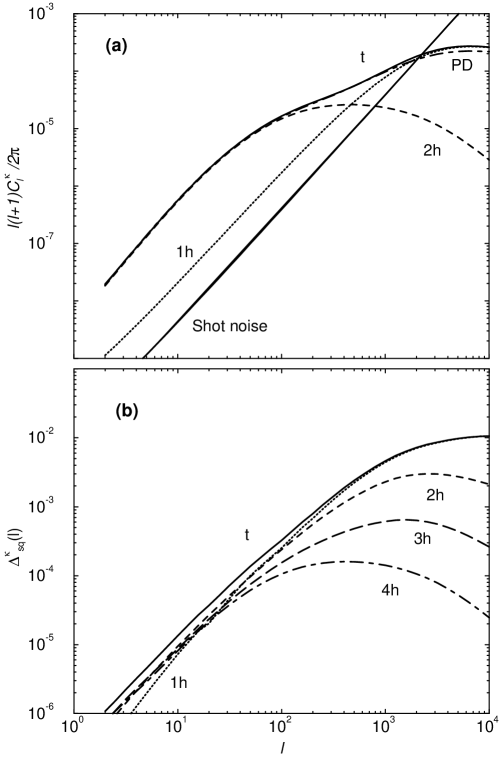
Figure 4.— Weak lensing convergence (a) power spectrum and (b) trispectrum under the halo description. Also shown in (a) is the prediction from the PD nonlinear power spectrum fitting function. We have separated individual contributions under the halo approach and have assumed that all sources are at $z_{s}=1$. We have also shown the shot noise contribution to the power spectrum assuming a survey down to a limiting magnitude of R $\sim$ 25 with an intrinsic rms shear of 0.4 in each component.

2.3.2 Comparisons

In Fig. 1(a), we show the logarithmic power spectrum $\Delta^{2}(k)=k^{3}P(k)/2\pi^{2}$ with contributions broken down to the $1h$ and $2h$ terms today and the $1h$ term at redshift of 1. We find that there is an slight overprediction of power at scales corresponding to $1\lesssim k\lesssim 10$ h Mpc${}^{-1}$ when compared to the PeaDod96 (1996) fitting function shown for redshifts of 0 and 1, and a more substantial underprediction at small scales with $k\gtrsim 10$ h Mpc${}^{-1}$. Since the non-linear power spectrum has only been properly studied out to overdensities $\Delta^{2}\sim 10^{3}$ with numerical simulations it is unclear whether the small-scale disagreement is significant. Fortunately, it is on sufficiently small scales so as not to affect the lensing observables.

For the trispectrum, we are mainly interested in terms involving $T({\bf k}_{1},-{\bf k}_{1},{\bf k}_{2},-{\bf k}_{2})$, i.e. parallelograms which are defined by either the length $k_{12}$ or the angle between ${\bf k}_{1}$ and ${\bf k}_{2}$. For illustration purposes we will take $k_{1}=k_{2}$ and the angle to be $90^{\circ}$ (${\bf k}_{2}={\bf k}_{\perp}$) such that the parallelogram is a square. It is then convenient to define

$$\Delta^{2}_{\rm sq}(k)\equiv\frac{k^{3}}{2\pi^{2}}T^{1/3}({\bf k},-{\bf k},{\bf k}_{\perp},-{\bf k}_{\perp})\,,$$ (28)

such that this quantity scales roughly as the logarithmic power spectrum itself $\Delta^{2}(k)$. This spectrum is shown in Fig. 1(b) with the individual contributions from the 1h, 2h, 3h, 4h terms shown. We test the sensitivity of our calculations to the width of the distribution in Fig. 2, where we show the ratio between single halo contribution, as a function of the concentration distribution width, to the halo term with a delta function distribution $\sigma_{c}=0$. As in the power spectrum the effect of increasing the width is to increase the amplitude at small scales due to the high concentration tail of the distribution. Notice that the width effect is stronger in the trispectrum than the power spectrum since the tails of the distribution are weighted more heavily in higher point statistics.

To compare the specific scaling predicted by perturbation theory in the linear regime and the hierarchical ansatz in the deeply non-linear regime, it is useful to define the quantity

$$Q_{\rm sq}(k)\equiv\frac{T({\bf k},-{\bf k},{\bf k}_{\perp},-{\bf k}_{\perp})}{[8P^{2}(k)P(\sqrt{2}k)][4P^{3}(k)]}\,.$$ (29)

In the halo prescription, $Q_{\rm sq}$ at $k\gtrsim 10k_{\rm nonlin}\sim 10h$Mpc${}^{-1}$ arises mainly from the single halo term. In perturbation theory $Q_{\rm sq}\approx 0.085$. The $Q_{\rm sq}$ does not approach the perturbation theory prediction as $k\rightarrow 0$ since that contribution appears only as one term in the 4 halo piece. There is an intrinsic shot noise error introduced by modeling the continuous density field by discrete objects. This error appears large in the $Q_{\rm sq}$ statistic since we have subtracted out the much larger connected (Gaussian) piece of the four point function. For example in the power spectrum covariance, the error induced by this approximation is much less than the Gaussian variance.

The hierarchical ansatz predicts that $Q_{\rm sq}=$ const. in the deeply non-linear regime. Its value is unspecified by the ansatz but is given as

$$Q_{\rm sq}^{\rm sat}=\frac{1}{2}\left[\frac{54-27\cdot 2^{n}+2\cdot 3^{n}+6^{n}}{1+6\cdot 2^{n}+3\cdot 3^{n}+6\cdot 6^{n}}\right]$$ (30)

under hyperextended perturbation theory (HEPT; ScoFri99). Here $n=n(k)$ is the linear power spectral index at $k$. As shown in Fig. 3, the halo model predicts $Q_{\rm sq}$ increases at high $k$. This behavior, also present at the three point level for the dark matter density field bispectrum, suggests disagreement between the halo approach and hierarchical clustering ansatz (see, MaFry00b 2000b), though numerical simulations do not yet have enough resolution to test this disagreement. Fortunately the discrepancy is also outside of the regime important for lensing.

To further test the accuracy of our halo trispectrum, we compare dark matter correlations predicted by our method to those from numerical simulations by MeiWhi99 (1999). For this purpose, we calculate the covariance matrix $C_{ij}$ from Eqn. (5) with the bins centered at $k_{i}$ and volume $V_{{\rm s}i}=4\pi k_{i}^{2}\delta{k_{i}}$ corresponding to their scheme. We also employ the parameters of their $\Lambda$CDM cosmology and assume that the parameters that defined the halo concentration properties from our fiducial $\Lambda$CDM model holds for this cosmological model also. The physical differences between the two cosmological model are minor, though normalization differences can lead to large changes in the correlation coefficients.

In Table 1, we compare the predictions for the correlation coefficients

$$\hat{C}_{ij}={C_{ij}\over\sqrt{C_{ii}C_{jj}}}$$ (31)

with the simulations. Agreement in the off diagonal elements is typically better than $\pm 0.1$, even in the region where non-Gaussian effects dominate, and the qualitative features such as the increase in correlations across the non-linear scale are preserved.

A further test on the accuracy of the halo approach is to consider higher order real-space moments such as skewness and kurtosis. In CooHu00 (2000), we discussed the weak lensing convergence skewness under the halo model and found it to be in agreement with numerical predictions from WhiHu99 (1999). The fourth moment of the density field, under certain approximations, was calculated by Scoetal99 (1999) using dark matter halos and was found to be in good agreement with N-body simulations. Given that density field moments have already been studied by Scoetal99, we no longer consider them here other than to suggest that the halo model has provided, at least qualitatively, a consistent description better than any of the perturbation theory arguments.

Even though the dark matter halo formalism provides a physically motivated means of calculating the statistics of the dark matter density field, and especially higher order correlations, there are several limitations of the approach that should be borne in mind when interpreting results. The approach assumes all halos to share a parameterized spherically-symmetric profile. We have attempted to include variations in the halo profiles with the addition of a distribution function for concentration parameter based on results from numerical simulations. Unlike our previous calculations presented in Cooetal00 (2000) and CooHu00 (2000), we have not modified concentration-mass relation to fit the PD non-linear power spectrum, but rather have taken results directly from simulations as inputs. Though we have partly accounted for halo profile variations, the assumption that halos are spherical is likely to affect detailed results on the configuration dependence of the trispectrum. Since we are considering a weighted average of configurations, our tests here are insufficient to establish the validity of the trispectrum modeling in general. Further numerical work is required to quantify to what extent the present approach reproduces simulation results for the full trispectrum.

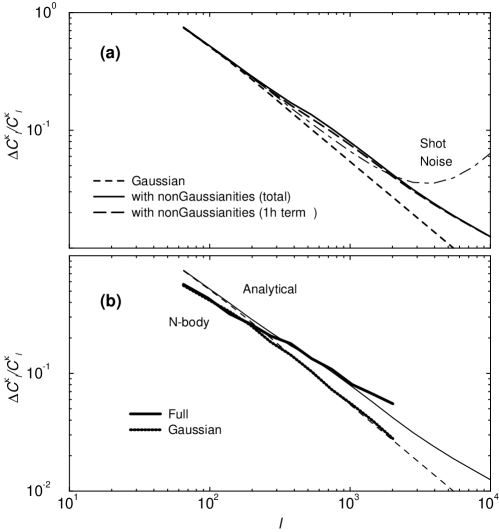
Figure 5.— The fractional errors in the measurements of the convergence band powers. In (a), we show the fractional errors under the Gaussian approximation, the full halo description, the Gaussian plus single halo term, and the Gaussian plus shot noise term (see §3.3). As shown, the additional variance can be modeled with the single halo piece while shot noise generally becomes dominant before non-Gaussian effects become large. In (b), we compare the halo model with simulations from WhiHu99 (1999). The decrease in the variance at small $l$ in the simulations is due to the conversion of variance to covariance by the finite box size of the simulations.

Table 2

Weak Lensing Convergence Power Spectrum Correlations
$\ell_{\rm bin}$ 97 138 194 271 378 529 739 1031 1440 2012 97 1.00 0.04 0.05 0.07 0.08 0.09 0.09 0.09 0.08 0.08 138 (0.26) 1.00 0.08 0.10 0.11 0.12 0.12 0.12 0.11 0.11 194 (0.12) (0.31) 1.00 0.14 0.17 0.18 0.18 0.17 0.16 0.15 271 (0.10) (0.21) (0.26) 1.00 0.24 0.25 0.25 0.24 0.22 0.21 378 (0.02) (0.09) (0.24) (0.38) 1.00 0.33 0.33 0.32 0.30 0.28 529 (0.10) (0.14) (0.28) (0.33) (0.45) 1.00 0.42 0.40 0.37 0.35 739 (0.12) (0.16) (0.17) (0.34) (0.38) (0.50) 1.00 0.48 0.45 0.42 1031 (0.15) (0.18) (0.15) (0.27) (0.33) (0.48) (0.54) 1.00 0.52 0.48 1440 (0.18) (0.15) (0.19) (0.19) (0.32) (0.36) (0.53) (0.57) 1.00 0.54 2012 (0.19) (0.22) (0.16) (0.32) (0.27) (0.46) (0.50) (0.61) (0.65) 1.00

NOTES.—Covariance of the binned power spectrum when sources are at a redshift of 1. Upper triangle displays the covariance found under the halo model. Lower triangle (parenthetical numbers) displays the covariance found in numerical simulations by WhiHu99 (1999). To be consistent with these simulations, we use the same binning scheme as the one used there.

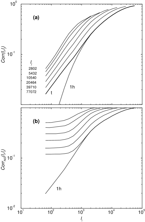
Figure 6.— (a) The correlation coefficient, $\hat{C}_{ij}$ as a function of the multipole $l_{i}$ with $l_{j}$ as shown in the figure. We show the correlations calculated with the full halo model and also with only the single halo term for $l_{j}=77072$. In (b), we show the non-Gaussian correlation coefficient $\hat{C}_{ij}^{\rm NG}$, which only involves the trispectrum (see, Eq. 42). The transition to full correlation is due to the domination of the single halo contribution.

3. Convergence Power Spectrum Covariance

3.1. General Definitions

Weak lensing probes the statistical properties of the shear field on the sky which is a weighted projection of the matter distribution along the line of sight to the source galaxies. As such, the observables may be reexpressed as a scalar quantity, the convergence $\kappa$, on the sky.

Its power spectrum and trispectrum are defined in the flat sky approximation in the usual way

$$\left<\kappa({\mathbf{l}}_{1})\kappa({\mathbf{l}}_{2})\right> = (2\pi)^{2}\delta_{\rm D}({\mathbf{l}}_{12})C_{l}^{\kappa}\,,$$

$$\left<\kappa({\mathbf{l}}_{1})\ldots\kappa({\mathbf{l}}_{4})\right>_{c} = (2\pi)^{2}\delta_{\rm D}({\mathbf{l}}_{1234})T^{\kappa}({\mathbf{l}}_{1},{\mathbf{l}}_{2},{\mathbf{l}}_{3},{\mathbf{l}}_{4})\,.$$ (32)

These are related to the density power spectrum and trispectrum by the projections (Kai92 1992; Scoetal99 1999)

$$C^{\kappa}_{l} = \int dr\frac{W(r)^{2}}{d_{A}^{2}}P\left(\frac{l}{d_{A}};r\right)\,,$$ (33)

$$T^{\kappa} = \int dr\frac{W(r)^{4}}{d_{A}^{6}}T\left(\frac{{\mathbf{l}}_{1}}{d_{A}},\frac{{\mathbf{l}}_{2}}{d_{A}},\frac{{\mathbf{l}}_{3}}{d_{A}},\frac{{\mathbf{l}}_{4}}{d_{A}},;r\right)\,,$$ (34)

where $r$ is the comoving distance and $d_{A}$ is the angular diameter distance. When all background sources are at a distance of $r_{s}$, the weight function becomes

$$W(r)=\frac{3}{2}\Omega_{m}\frac{H_{0}^{2}}{c^{2}a}\frac{d_{A}(r)d_{A}(r_{s}-r)}{d_{A}(r_{s})}\,;$$ (35)

for simplicity, we will assume $r_{s}=r(z_{s}=1)$. In deriving Eq. (34), we have used the Limber approximation (Lim54 1954) by setting $k=l/d_{A}$ and the flat-sky approximation. A potential problem in using the Limber approximation is that we implicitly integrate over the unperturbed photon paths (Born approximation). The Born approximation has been tested in numerical simulations by JaiSelWhi00 (2000; see their Fig. 7) and found to be an excellent approximation for the two point statistics. The same approximation can also be tested through lens-lens coupling involving lenses at two different redshifts. For higher order correlations, analytical calculations in the mildly non-linear regime by vanetal00 (2000b; also, Beretal97 1997; Schetal98 1998) indicate that corrections are again less than a few percent. Thus, our use of the Limber approximation by ignoring the lens-lens coupling is not expected to change the final results significantly.

For the purpose of this calculation, we assume that upcoming weak lensing convergence power spectrum will measure binned logarithmic band powers at several $l_{i}$’s in multipole space with bins of thickness $\delta l_{i}$.

$${\cal C}_{i}=\int_{{\rm s}i}{d^{2}l\over{A_{{\rm s}i}}}\frac{l^{2}}{2\pi}\kappa(\bf l)\kappa(-\bf l)\,,$$ (36)

where $A_{\rm s}(l_{i})=\int d^{2}l$ is the area of 2D shell in multipole and can be written as $A_{\rm s}(l_{i})=2\pi l_{i}\delta l_{i}+\pi(\delta l_{i})^{2}$.

We can now write the signal covariance matrix as

$$C_{ij} = {1\over A}\left[{(2\pi)^{2}\over A_{{\rm s}i}}2{\cal C}_{i}^{2}+T^{\kappa}_{ij}\right]\,,$$ (37)

$$T^{\kappa}_{ij} = \int{d^{2}l_{i}\over A_{{\rm s}i}}\int{d^{2}l_{j}\over A_{{\rm s}j}}{l_{i}^{2}l_{j}^{2}\over(2\pi)^{2}}T^{\kappa}({\mathbf{l}}_{i},-{\mathbf{l}}_{i},{\mathbf{l}}_{j},-{\mathbf{l}}_{j})\,,$$ (38)

where $A$ is the area of the survey in steradians. Again the first term is the Gaussian contribution to the sample variance and the second the non-Gaussian contribution. A realistic survey will also have shot noise variance due to the finite number of source galaxies in the survey. We will return to this point in the §3.3.

3.2. Comparisons

Table 3

Inverse Fisher Matrix ($\times$ 10${}^{3}$) $p_{i}$ $\Omega_{\Lambda}$ $\ln$ A $\Omega_{K}$ $n_{s}$ $\Omega_{m}h^{2}$ $\Omega_{\Lambda}$ 1.57 -5.96 -1.39 4.41 -1.76 $\ln$ A 25.89 5.83 -17.34 6.74 $\Omega_{K}$ 1.41 -3.81 1.43 $n_{s}$ 14.01 -6.03 $\Omega_{m}h^{2}$ 2.67 $p_{i}$ $\Omega_{\Lambda}$ $\ln$ A $\Omega_{K}$ $n_{s}$ $\Omega_{m}h^{2}$ $\Omega_{\Lambda}$ 2.03 -7.84 -1.82 5.76 -2.30 $\ln$ A 33.92 7.65 -22.79 8.91 $\Omega_{K}$ 1.78 -5.01 1.95 $n_{s}$ 18.43 -7.85 $\Omega_{m}h^{2}$ 3.44

NOTES.—Inverse Fisher matrix under the Gaussian assumption (top) and the halo model (bottom). The error on an individual parameter is the square root of the diagonal element of the Fisher matrix for the parameter while off-diagonal entries of the inverse Fisher matrix shows correlations, and, thus, degeneracies, between parameters. We have assumed a full sky survey ($f_{\rm sky}=1$) with parameters as described in § 3.3.

Using the halo model, we can now calculate contributions to lensing convergence power spectrum and trispectrum. The logarithmic power spectrum, shown in Fig. 4(a), shows the same behavior as the density field when compared with the PD results: a slight overprediction of power when $l\gtrsim 10^{3}$. However, these differences are not likely to be observable given the shot noise from the finite number of galaxies at small scales.

In Fig 4(b), we show the scaled trispectrum

$$\Delta^{\kappa}_{\rm sq}(l)=\frac{l^{2}}{2\pi}T^{\kappa}({\bf l},-{\bf l},{\bf l}_{\perp},-{\bf l}_{\perp})^{1/3}\,.$$ (39)

where $l_{\perp}=l$ and ${\bf l}\cdot{\bf l}_{\perp}=0$. The projected lensing trispectrum again shows the same behavior as the density field trispectrum with similar conditions on ${\bf k}_{i}$’s.

We can now use this trispectrum to study the contributions to the covariance, which is what we are primarily concerned here. In Fig. 5a, we show the fractional error,

$${\Delta{\cal C}_{i}\over{\cal C}_{i}}\equiv{\sqrt{C_{ii}}\over{\cal C}_{i}}\,,$$ (40)

for bands $l_{i}$ given in Table 2 following the binning scheme used by WhiHu99 (1999) on $6^{\circ}\times 6^{\circ}$ fields. The dashed line compares that with the Gaussian errors, involving the first term in the covariance (Eq. 38). At multipoles of a few hundred and greater, the non-Gaussian term begins to dominate the contributions. For this reason, the errors are well approximated by simply taking the Gaussian and single halo contributions.

In Fig. 5b, we compare these results with those of the WhiHu99 (1999) simulations. The decrease in errors from the simulations at small $l$ reflects finite box effects that convert variance to covariance as the fundamental mode in the box becomes comparable to the bandwidth.

The correlation between the bands is given by

$$\hat{C}_{ij}\equiv\frac{C_{ij}}{\sqrt{C_{ii}C_{jj}}}\,.$$ (41)

In Table 2 we compare the halo predictions to the simulations by WhiHu99 (1999). The upper triangle here is the correlations under the halo approach, while the lower triangle shows the correlations found in numerical simulations. The correlations along individual columns increase (as one goes to large $l$’s or small angular scales) consistent with simulations. In Fig. 6, we show the correlation coefficients with (a) and without (b) the Gaussian contribution to the diagonal.

We show in Fig. 6(a) the behavior of the correlation coefficient between a fixed $l_{j}$ as a function of $l_{i}$. When $l_{i}=l_{j}$ the coefficient is 1 by definition. Due to the presence of the dominant Gaussian contribution at $l_{i}=l_{j}$, the coefficient has an apparent discontinuity between $l_{i}=l_{j}$ and $l_{i}=l_{j-1}$ that decreases as $l_{j}$ increases and non-Gaussian effects dominate.

To better understand this behavior it is useful to isolate the purely non-Gaussian correlation coefficient

$$\hat{C}^{\rm NG}_{ij}=\frac{T_{ij}}{\sqrt{T_{ii}T_{ij}}}\,.$$ (42)

As shown in Fig. 6(b), the coefficient remains constant for $l_{i}\ll l_{j}$ and smoothly increases to unity across a transition scale that is related to where the single halo terms starts to contribute. A comparison of Fig. 6(b) and 4(b), shows that this transition happens around $l$ of few hundred to 1000. Once the power spectrum is dominated by correlations in single halos, the fixed profile of the halos will correlate the power in all the modes. The multiple halo terms on the other hand correlate linear and non-linear scales but at a level that is generally negligible compared with the Gaussian variance.

The behavior seen in the halo based covariance, however, is not present when the covariance is calculated with hierarchical arguments for the trispectrum (see, Scoetal99 1999). With hierarchical arguments, which are by construction only valid in the deeply nonlinear regime, one predicts correlations which are, in general, constant across all scales and shows no decrease in correlations between very small and very large scales. Such hierarchical models also violate the Schwarz inequality with correlations greater than 1 between large and small scales (e.g., Scoetal99 1999; Ham00 2000). The halo model, however, shows a decrease in correlations similar to numerical simulations suggesting that the halo model, at least qualitatively, provides a better approach to studing non-Gaussian correlations in the translinear regime.

3.3. Effect on Parameter Estimation

Modeling or measuring the covariance matrix of the power spectrum estimates will be essential for interpreting observational results. In the absence of many fields where the covariance can be estimated directly from the data, the halo model provides a useful, albeit model dependent, quantification of the covariance. As a practical approach one could imagine taking the variances estimated from the survey under a Gaussian approximation, but which accounts for uneven sampling and edge effects (HuWhi00 2000), and scaling it up by the non-Gaussian to Gaussian variance ratio of the halo model along with inclusion of the band power correlations. Additionally, it is in principle possible to use the expected correlations from the halo model to decorrelate individual band power measurements, similar to studies involving CMB temperature anisotropy and galaxy power spectra (e.g., Ham97 1997; HamTeg00 2000).

We can estimate the resulting effects on cosmological parameter estimation with an analogous procedure on the Fisher matrix. In HuTeg99 (1999), the potential of wide-field lensing surveys to measure cosmological parameters was investigated using the Gaussian approximation of a diagonal covariance and Fisher matrix techniques. The Fisher matrix is simply a projection of the covariance matrix onto the basis of cosmological parameters $p_{i}$

$${\bf F}_{\alpha\beta}=\sum_{ij}{\partial{\cal C}_{i}\over\partial p_{\alpha}}(C_{\rm tot}^{-1})_{ij}{\partial{\cal C}_{j}\over\partial p_{\beta}}\,,$$ (43)

where the total covariance includes both the signal and noise covariance. Under the approximation of Gaussian shot noise, this reduces to replacing $C^{\kappa}_{l}\rightarrow C^{\kappa}_{l}+C^{\rm SN}_{l}$ in the expressions leading up to the covariance equation (38). The shot noise power spectrum is given by

$$C^{\rm SN}_{l}=\frac{\langle\gamma_{\rm int}^{2}\rangle}{\bar{n}}\,,$$ (44)

where $\langle\gamma_{\rm int}\rangle^{1/2}\sim 0.4$ is the rms noise per component introduced by intrinsic ellipticities and measurement errors and $\bar{n}\sim 6.6\times 10^{8}$ sr${}^{-1}$ is the surface number density of background source galaxies. The numerical values here are appropriate for surveys that reach a limiting magnitude in $R\sim 25$ (e.g., Smaetal95 1995).

Under the approximation that there are a sufficient number of modes in the band powers that the distribution of power spectrum estimates is approximately Gaussian, the Fisher matrix quantifies the best possible errors on cosmological parameters that can be achieved by a given survey. In particular $F^{-1}$ is the optimal covariance matrix of the parameters and $(F^{-1})_{ii}^{1/2}$ is the optimal error on the $i$th parameter. Implicit in this approximation of the Fisher matrix is the neglect of information from the cosmological parameter dependence of the covariance matrix of the band powers themselves. Since the covariance is much less than the mean power, we expect this information content to be small.

In order to estimate the effect of non-Gaussianities on the cosmological parameters, we calculate the Fisher matrix elements using our fiducial $\Lambda$CDM cosmological model and define the dark matter density field, today, as

$$\Delta^{2}(k)=A^{2}\left(\frac{k}{H_{0}}\right)^{n_{s}+3}T^{2}(k)\,.$$ (45)

Here, $A$ is the amplitude of the present day density fluctuations and $n_{s}$ is the tilt at the Hubble scale. The density power spectrum is evolved to higher redshifts using the growth function $G(z)$ (Pee80 1980) and the transfer function $T(k)$ is calculated using the fitting functions from EisHu99 (1999). Since we are only interested in the relative effect of non-Gaussianities, we restrict ourselves to a small subset of the cosmological parameters considered by HuTeg99 (1999) and assume a full sky survey with $f_{\rm sky}=1$.

In Table 3, we show the inverse Fisher matrices determined under the Gaussian and non-Gaussian covariances, respectively. For the purpose of this calculation, we adopt the binning scheme as shown in Table 2, following WhiHu99 (1999). The Gaussian errors are computed using the same scheme by setting $T^{\kappa}=0$. As shown in Table 3, the inclusion of non-Gaussianities lead to an increase in the inverse Fisher matrix elements. We compare the errors on individual parameters, mainly $(F^{-1})_{ii}^{1/2}$, between the Gaussian and non-Gaussian assumptions in Table 4. The errors increase typically by $\sim 15$%. Note also that band power correlations do not necessarily increase cosmological parameter errors. Correlations induced by non-linear gravity introduce larger errors in the overall amplitude of the power spectrum measuremenents but have a much smaller effect on those parameters controlling the shape of the spectrum.

For a survey of this assumed depth, the shot noise power becomes the dominant error before the non-Gaussian signal effects dominate over the Gaussian ones. For a deeper survey with better imaging, such as the one planned with Large-aperture Synoptic Survey Telescope (LSST; TysAng00 2000), the effect of shot noise decreases and non-Gaussianity is potentially more important. However, the non-Gaussianity itself also decreases with survey depth, and as we now discuss, in terms of the effect of non-Gaussianities, deeper surveys should be preferred over the shallow ones.

3.4. Scaling Relations

To better understand how the non-Gaussian contribution scale with our assumptions, we consider the ratio of non-Gaussian variance to the Gaussian variance (Scoetal99 1999),

$$\frac{C_{ii}}{C_{ii}^{\rm G}}=1+R\,,$$ (46)

with

$$R\equiv\frac{A_{si}T_{ii}^{\kappa}}{(2\pi)^{2}2C_{i}^{2}}\,.$$ (47)

Under the assumption that contributions to lensing convergence can be written through an effective distance $r_{\star}$, at half the angular diameter distance to background sources, and a width $\Delta r$ for the lensing window function, the ratio of lensing convergence trispectrum and power spectrum contribution to the variance can be further simplified to

$$R\sim\frac{A_{si}}{V_{\rm eff}}\frac{\bar{T}(r_{\star})}{\bar{P}^{2}(r_{\star})}\,.$$ (48)

Since the lensing window function peaks at $r_{\star}$, we have replaced the integral over the window function of the density field trispectrum and power spectrum by its value at the peak. This ratio shows how the relative contribution from non-Gaussianities scale with survey parameters: (a) increasing the bin size, through $A_{si}$ ($\propto\delta l$), leads to an increase in the non-Gaussian contribution linearly, (b) increasing the source redshift, through the effective volume of lenses in the survey ($V_{\rm eff}\sim r_{\star}^{2}\Delta r$), decreases the non-Gaussian contribution, while (c) the growth of the density field trispectrum and power spectrum, through the ratio $\bar{T}/\bar{P}^{2}$, decreases the contribution as one moves to a higher redshift. The volume factor quantifies the number of foreground halos in the survey that effectively act as gravitational lenses for background sources; as the number of such halos is increased, the non-Gaussianities are reduced by the central limit theorem.

In order to determine whether its the increase in volume or the decrease in the growth of structures that lead to a decrease in the relative importance of non-Gaussianities as one moves to a higher source redshift, we numerically calculated the non-Gaussian to Gaussian variance ratio under the halo model for several source redshifts and survey volumes. Up to source redshifts $\sim$ 1.5, the increase in volume decreases the non-Gaussian contribution significantly. When surveys are sensitive to sources at redshifts beyond 1.5, the increase in volume becomes less significant and the decrease in the growth of structures begin to be important in decreasing the non-Gaussian contribution. Since, in the deeply non-linear regime, $\bar{T}/\bar{P}^{2}$ scales with redshift as the cube of the growth factor, this behavior is consistent with the overall redshift scaling of the volume and growth.

Given that scalings always lead to decrease the effect of non-Gaussianities in deep lensing surveys, with a decrease in the shot noise contribution also, shallow surveys that only probe sources out to redshifts of a few tenths are more likely to be dominated by non-Gaussianities; such shallow surveys are also likely to be affected by intrinsic correlations of galaxy shapes (e.g., Catetal00 2000; CroMet00 2000; Heaetal00 2000). These possibilities, generally, suggests that deeper surveys should be preferred over shallow ones for weak lensing purposes.

Table 4

Parameter Errors $\Omega_{\Lambda}$ $\ln$ A $\Omega_{k}$ $n_{s}$ $\Omega_{m}h^{2}$ Gaussian 0.039 0.160 0.037 0.118 0.051 Full 0.045 0.184 0.042 0.135 0.058 Increase (%) 15.3 15 13.5 14.4 13.7

NOTES.—Parameter errors, $(F^{-1})_{ii}^{1/2}$, under the Gaussian assumption (top) and the halo model (bottom) and following the inverse-Fisher matrices in Table 3. We have assumed a full sky survey ($f_{\rm sky}=1$) with parameters as described in § 3.3.