Numerical and Analytical Predictions for the Large-Scale Sunyaev-Zel’dovich Effect

Abstract

The hot gas embedded in the large-scale structures in the Universe produces secondary fluctuations in the Cosmic Microwave Background (CMB). Because it is proportional to the gas pressure integrated along the line of sight, this effect, the thermal Sunyaev-Zel’dovich (SZ) effect, provides a direct measure of large-scale structure and of cosmological parameters. We study the statistical properties of this effect using both hydrodynamical simulations and analytical predictions from an extended halo model. The Adaptive Mesh Refinement scheme, used in the newly developed code RAMSES, provides a dynamic range of 4 order of magnitudes, and thus allows us to significantly improve upon earlier calculations. After accounting for the finite mass resolution and box size of the simulation, we find that the halo model agrees well with the simulations. We discuss and quantify the uncertainty in both methods, and thus derive an accurate prediction for the SZ power spectrum in the $10^{2}\lesssim l\lesssim 10^{5}$ range of multipole. We show how this combined analytical and numerical approach is essential for accuracy, and useful for the understanding of the physical processes and scales which contribute to large-scale SZ anisotropies.

I Introduction

The hot gas in the IGM induces distortions in the spectrum of the Cosmic Microwave Background (CMB) through the Sunyaev-Zel’dovich (SZ) effect [1, 2]. This effect is proportional to the integrated electron pressure along the line-of-sight and can be directly measured by mapping the anisotropies of the CMB (see [3, 4] for reviews). It acts as a foreground for the measurement of primary anisotropies of the CMB (see eg. [5] for a review), and is a direct probe of large-sale structure and of the distribution of baryons in the universe. This technique is now well established for the study of individual clusters of galaxies (eg. [3, 4, 6, 7]). A more complete and unbiased statistical description of the SZ effect requires wide field surveys, and will soon be achieved by upcoming and future CMB experiments (see [8, 9, 32] and reference therein). In this perspective, accurate theoretical predictions of the statistics of the large-scale SZ effect are necessary.

The statistics of SZ anisotropies have been studied using various methods. Scaramella et al. [13], and more recently da Silva et al. [14, 15] and Seljak, Burwell & Pen [20], have used numerical simulations to construct SZ maps and study their statistical properties. Persi et al. [16] and Refregier et al. [19] used instead a semi-analytical method, consisting of computing the SZ angular power spectrum by projecting the 3-dimensional power spectrum of the gas pressure on the sky. Aghanim et al. [8], Atrio-Barandela & Mücket [11] and Komatsu & Kitayama [12] used the Press & Schechter formalism [35] to predict the SZ power spectrum in various CDM models. In the same spirit, Cooray [21] recently used a self-consistent extended halo model [30, 29] to make analytical predictions for the large-scale SZ effect. In a different approach, Zhang & Pen [22] recently presented analytical predictions based on hierarchical clustering and non-linear perturbation theory.

The accuracy of these different predictions are limited both by the limited dynamical range of the simulations and the lack of detailed comparison between the numerical and analytical methods. In this paper, we combine the approaches of Refregier et al. [19] and of Cooray [21] to carefully compare predictions from numerical simulations to that from the extended halo model. We use a recently developed Adaptative Mesh Refinement (AMR) hydrodynamical code, called RAMSES (see Teyssier [23] for a complete presentation), to compute the power spectrum of the gas pressure and of the Dark Matter (DM) density in a $\Lambda$CDM universe. The AMR simulations provide a dynamic range of 4 orders of magnitude and thus allow us to significantly improve upon earlier calculations. After ensuring the proper treatment of the DM power spectrum, the extended halo model allows us to predict the gas-pressure power spectrum without additional free parameter. We compare the predictions from both methods in detail, and pay particular attention to the limitations imposed by finite mass resolution and box size. We then compute the resulting SZ power spectrum and discuss the reliability and accuracy of our prediction.

This paper is organized as follows. In §II, we briefly describe the SZ effect and derive expressions for the integrated comptonization parameter and the SZ power spectrum. In §III, we describe the halo model for the DM and the baryons. In §IV, we describe the numerical methods used for the RAMSES simulations. In §V we present the comparative results for the DM power spectrum, the evolution of the density-weighted temperature, the pressure power spectrum and the SZ power spectrum. Our conclusions are summarized in §VI.

II Sunyaev–Zel’dovich Effect

The thermal SZ effect is produced from the inverse Compton scattering of CMB photons by the hot electrons in the IGM [1, 2, 3, 4]. The first SZ observable is the mean comptonization parameter which can be measured from the distortion of the CMB Planck spectrum (see [25] for a review). Following the conventions of [19], we find that it is given by

$$\overline{y}=y_{0}\int_{0}^{\chi_{i}}d\chi\overline{T}_{\rho}a^{-2}.$$ (1)

where $\chi$ is the comoving distance, $a$ is the expansion parameter and $y_{0}\simeq 1.710\times 10^{-16}\left(\frac{\Omega h^{2}}{0.05}\right)$ K^-1 Mpc^-1, for a He mass fraction of 0.24 and assuming thermal equilibrium between the ions and electrons. The limiting distance $\chi_{i}$ corresponds to the reionization redshift, for which recent theoretical studies suggest a value around $z_{i}\simeq 10$ [28]. The mean density-weighted temperature of the gas is proportional to the average pressure and is defined as

$$\overline{T}_{\rho}\equiv\langle\rho T\rangle/\langle\rho\rangle,$$ (2)

where $\rho$ and $T$ are the density and temperature of the gas, respectively.

The large-scale SZ effect can also be measured from the anisotropies that it induces on the CMB temperature. In the Rayleigh-Jeans (RJ) regime and in the small angle approximation, the angular power spectrum of these fluctuations is given by (see again [19] for conventions)

$$C_{\ell}\simeq 4y_{0}^{2}\int_{0}^{\chi_{i}}d\chi\overline{T}_{\rho}^{2}P_{p}\!\left(\frac{\ell}{r},\chi\right)a^{-4}r^{-2},$$ (3)

where $r$ is the comoving angular diameter distance, and $P_{p}(k,\chi)$ is the 3-dimensional power spectrum of the pressure fluctuations $\delta_{P}=(P-\langle P\rangle)/\langle P\rangle$ at comoving distance $\chi$. In the course of our work, we found that $\overline{y}$ is sensitive to the actual value of $z_{i}$, while the SZ power spectrum $C_{l}$ is almost insensitive to it. For definitiveness, we hitherto assume a fixed value for the reionization redshift of $z_{i}=10$.

III Halo model

A Dark Matter

To model the dark matter as a collection of halos, we follow the approach of Seljak [29] and of Ma & Fry [30]. Because its precise predictions depend on a number of assumptions, we here summarize the components of our halo model. The number of halos of mass M per unit comoving volumes and per unit mass at redshift $z$ is given by the mass function

$$\frac{dn}{dM}=\frac{\overline{\rho}}{M}\frac{d\nu}{dM}f(\nu),$$ (4)

where $\overline{\rho}$ is the average matter density. The peak height $\nu$ is defined as

$$\nu(M,z)\equiv\frac{\delta_{c}}{\sigma(M,z)}$$ (5)

where $\sigma(M,z)$ is the linear rms mass fluctuation in spheres of radius $R$ given by $M=4\pi\overline{\rho}R^{3}/3$ at redshift $z$. This quantity can be computed from the linear power spectrum $P_{\rm lin}(k,z)$, which we evaluate from the the BBKS transfer function [31] (with the conventions of [33]) evolved with the linear growth factor. The density threshold $\delta_{c}$ is equal to 1.68 in an Einstein-De Sitter universe, and has a weak cosmology dependence which we compute using the results of Kitayama & Suto [34]. We adopt the standard Press-Schechter formalism [35], which dictates

$$f(\nu)=\sqrt{\frac{2}{\pi}}e^{-\nu^{2}/2}.$$ (6)

In order for the halos to amount to the total mass density $\overline{\rho}$, the mass function must be normalized as

$$\frac{1}{\overline{\rho}}\int_{0}^{\infty}dM\frac{dn}{dM}M=\int_{0}^{\infty}d\nu f(\nu)=1.$$ (7)

This is formally satisfied by the Press & Schechter mass function, as soon as $\sigma(M,z)\rightarrow+\infty$ for $M\rightarrow 0$. However, in CDM-like model this divergence at small $M$’s is very slow, thus, practically, leaving a fraction of the mass in the background (i.e. not in collapsed halos). We account for this background mass by adding a constant to the mass function in our smallest mass bin (typically $10^{6}M_{\odot}$).

To each halo, we assign a Navarro, Frenk & White (NFW) mass density profile [36], which is given by

$$\rho(r)=\rho_{s}u(r/r_{s}),~{}~{}u(x)=x^{-1}(1+x)^{-2}$$ (8)

where $r$ is the comoving radius, $r_{s}$ and $\rho_{s}$ are the characteristic radius and density, respectively . These characteristic quantities can be written in terms of the virial radius $r_{v}$ within which the mean density contrast is $\delta_{v}=200$. Identifying the mass $M$ to the virial mass, we get $M=4\pi\overline{\rho}\delta_{v}r_{v}^{3}/3=4\pi\int_{0}^{r_{v}}drr^{2}\rho(r)$, yielding $\rho_{s}=\overline{\rho}\delta_{v}c^{3}\left[\ln(1+c)-c/(1+c)\right]^{-1}/3$. In the previous expression, we have used the compactness parameter which is defined as

$$c(M,z)\equiv r_{v}/r_{s}.$$ (9)

For the $\Lambda$ CDM model we consider here, we adopt the functional form of $c$ given by [32, 21]

$$c(M,z)\simeq g(z)\left[\frac{M}{M_{*}(z)}\right]^{-h(z)},$$ (10)

where $g(z)\simeq 10.3(1+z)^{-0.3}$ and $h(z)\simeq 0.24(1+z)^{-0.3}$. Here, $M_{*}(z)$ is the non-linear mass scale defined by $\nu(M_{*},z)\equiv 1$. The bias for the clustering of the halos is given by the Mo & White formalism [37], namely by

$$b(M,z)=1+\frac{\nu^{2}-1}{\delta_{c}}.$$ (11)

Assuming that the matter distribution can be modeled as a collection of these halos, the matter power spectrum is given by [29, 30]

$$P(k,z)=P_{1}(k,z)+P_{2}(k,z),$$ (12)

where the terms correspond the 1-halo (Poisson) and 2-halo (clustering) contribution. They are given by

$$P_{1}(k)=\int_{0}^{\infty}dM~{}\frac{dn}{dM}\left[\frac{\tilde{\rho}(k,M)}{\overline{\rho}}\right]^{2}$$ (13)

and

$$P_{2}(k)=\left[\int_{0}^{\infty}dM~{}\frac{dn}{dM}b(M)\frac{\tilde{\rho}(k,M)}{\overline{\rho}}\right]^{2}P_{\rm lin}(k)$$ (14)

where the radial Fourier transform of the density profile is given by

$$\tilde{\rho}(k,M)=4\pi\int_{0}^{r_{v}}dr~{}r^{2}\rho(r,M)\frac{\sin kr}{kr}.$$ (15)

Conveniently, $\tilde{\rho}(0)=M$. As noted by Seljak [29], the fact that on large scales $P(k)$ must approach $P_{lin}(k)$ imposes the non-trivial constraint

$$\frac{1}{\overline{\rho}}\int_{0}^{\infty}dM~{}\frac{dn}{dM}Mb(M)=\int_{0}^{\infty}d\nu~{}f(\nu)b(\nu)=1,$$ (16)

which formally holds in the case $\sigma(M,z)\rightarrow+\infty$ for $M\rightarrow 0$. As for the mass function, we practically force this normalization to be numerically exact by adding a constant to $b(M)$ in our smallest-mass bin.

The resulting power spectra at different redshifts are shown on Figure 1 for the $\Lambda$CDM model (with parameters listed in §IV B). Also shown are the power spectra from the Peacock & Dodds [38] fitting formula. As noted by [32], the agreement is good for all redshifts. Note that the only tuning involved is that of the functional form of the compactness parameter $c(M,z)$ (Eq. [10]).

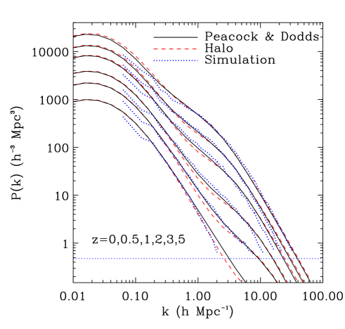
FIG. 1.: Power spectrum of the DM density at different redshifts for the $\Lambda$CDM model. The solid, dashed and dotted curves correspond to the Halo model, the Peacock & Dodds fit, and the simulations, respectively. The thin horizontal dotted line corresponds to the Poisson noise in the simulations.

B Virial Temperature

To model the baryons, we first consider the virial temperature of a halo which is given by

$$kT_{v}=\frac{G\mu m_{p}M}{2\beta_{v}r_{v,{\rm phys}}}\simeq 7.82(1+z)\beta_{v}^{-1}\Omega_{m}^{\frac{1}{3}}\left(\frac{M}{10^{15}h^{-1}M_{\odot}}\right)^{\frac{2}{3}}\left(\frac{\mu}{0.59}\right)\left(\frac{\Delta_{c}}{178}\right)^{\frac{1}{3}}{\rm keV},$$ (17)

where $r_{v,{\rm phys}}$ is the virial radius in physical coordinates and $\Delta_{c}(z,\Omega_{m},\Omega_{\Lambda})$ is the average virial overdensity which can be evaluated using the fitting formulae of [34]. The value $\mu=0.59$ (the number of particles per proton mass) corresponds to a hydrogen mass fraction of 76%. The factor $\beta_{v}$ is exactly equal to 1 for a truncated singular isothermal sphere. In the general case, it can be considered as an unknown normalization parameter, whose exact value is determined using numerical simulations. Values of $\beta_{v}$ between $1$ and $1.2$ provide good fits to numerical simulations [39, 40]. Here, we adopt $\beta_{v}=1$.

Taking the gas temperature to be equal to the virial temperature, we can compute the density-weighted temperature (Eq. [2]) of the gas which is given by

$$\overline{T}_{\rho}=\frac{1}{\overline{\rho}}\int_{M_{\rm min}}^{M_{\rm max}}dM~{}\frac{dn}{dM}MT_{v},$$ (18)

where $M_{\rm min}$ and $M_{\rm max}$ are mass limits introduced to model the finite mass resolution and box size of our numerical simulation (see §IV C). Note that, to ensure proper normalization of the total DM density (Eq. [7]), this mass range is not used to compute the power spectrum of the DM density (Eq. [12]). The resulting redshift evolution of this temperature is plotted on Figure 2, for different mass ranges.

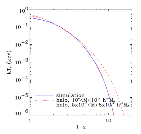
FIG. 2.: Evolution of the density-weighted temperature $\overline{T}_{\rho}$ of the gas. The prediction from the simulations is shown as the solid line. The prediction for the halo model is shown for different mass ranges $M_{\rm min}<M<M_{\rm max}$ as dashed and dotted lines.

C Gas Profile

To derive the profile of the gas pressure $p_{g}$ of halos, we further assume that the gas is in hydrostatic equilibrium and thus obeys

$$\frac{dp_{g}}{dr}=-\frac{G\rho_{g}(r)M(<r)}{r^{2}}$$ (19)

where $\rho_{g}$ is the gas density and $M(<r)$ is the total mass within radius $r$. Approximating the total mass as that of the Dark Matter only, it is easy to show that, for the NFW profile (Eq. [8]),

$$M(<r)=4\pi\rho_{s}r_{s}^{3}\left[\ln(1+\frac{r}{r_{s}})-\frac{r}{r+r_{s}}\right]$$ (20)

We need further assumptions to integrate Equation (19) for the pressure profile $p_{g}(r)$. As Cooray [21], we consider the simplest assumption, namely that the gas is ideal ($p_{g}=\frac{k_{B}}{\mu m_{p}}\rho_{g}T_{g}$) and isothermal within each halo, with a temperature equal to the virial temperature, i.e. $T_{g}(r)=T_{v}$. In this case, the hydrostatic equilibrium equation for the NFW mass profile yields

$$\rho_{g}(r)=\rho_{g0}v(r/r_{s},\lambda),~{}~{}~{}v(x,\lambda)=e^{-\lambda}(1+x)^{\frac{\lambda}{x}},$$ (21)

with

$$\lambda=\frac{4\pi\mu m_{p}G\rho_{s}r_{s}^{2}}{k_{B}T_{v}}.$$ (22)

This agrees with [21] up to a different power for $r_{s}$ in the last expression. The normalization $\rho_{g0}$ of the gas density profile is set by requiring that the baryon mass fraction is equal to that of the universe, i.e. by

$$M_{g}=4\pi\int_{0}^{r_{v}}dr~{}r^{2}\rho_{g}(r)=\frac{\Omega_{b}}{\Omega_{m}}M.$$ (23)

Following [21], we avoid an abrupt cutoff at the virial radius by multiplying the profile function $v(x)$ by an apodizing function which we choose to be $\left|E\left(\frac{x-c}{\sqrt{2}}\right)\right|$, where $E(x)$ is the error function.

In the limit of small radii, the gas density approaches $\rho_{g}(r)\propto e^{-\frac{r}{r_{g}}}$, where $r_{g}=\frac{2r_{s}}{\lambda}$ is the characteristic radius where the gas central density approaches a constant. It can be considered as a “core radius” in the gas distribution. The three characteristic radii $r_{v}$, $r_{s}$ and $r_{g}$ are plotted as a function of mass $M$ at $z=0$ and $z=3$ on figure 3. The inner radius $r_{g}$ scales roughly as $r_{s}$ with mass, but tends to increase as $z$ increases. This is due to the fact that, for a given mass, halos tend to have a higher temperature at high redshift (Eq. 17). In this model, the gas distribution is thus predicted to be more peaked at low redshift.

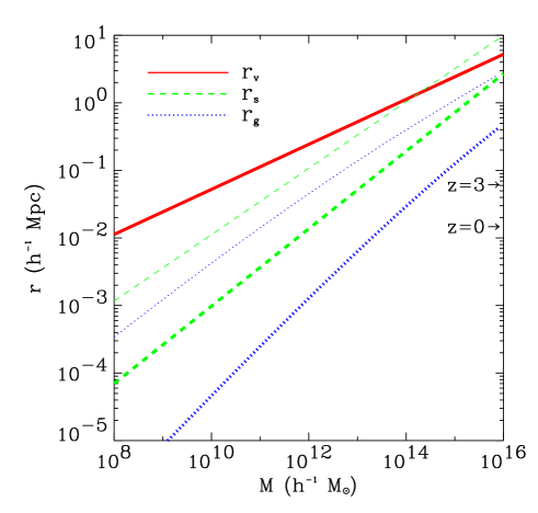
FIG. 3.: Characteristic comoving radii for the halo model as a function of halo mass. The virial radius $r_{v}$ (solid line), the NFW scale radius $r_{s}$ (dashed lines) and the gas inner radius $r_{g}$ (dotted lines) are all shown at $z=0$ (thick lines) and $z=3$ (thin lines). Note that the curves for the virial radius are identical for all redshifts. It is the interplay between these radii which determine the behavior of the gas pressure power spectrum on intermediate scales. We indicate by arrows the comoving spatial resolution of the numerical simulation at each redshift.

D Pressure Power Spectrum

As for the dark matter density (Eq. [12]), the pressure power spectrum $P_{p}(k)$ is related to the pressure profile by

$$P_{p}(k,z)=P_{p1}(k,z)+P_{p2}(k,z),$$ (24)

where 1-halo and 2-halo terms are given by

$$P_{p1}(k)=\int_{M_{\rm min}}^{M_{\rm max}}dM~{}\frac{dn}{dM}\left[\frac{\tilde{p}_{g}(k,M)}{\overline{p}_{g}}\right]^{2}$$ (25)

and

$$P_{p2}(k)=\left[\int_{M_{\rm min}}^{M_{\rm max}}dM~{}\frac{dn}{dM}b(M)\frac{\tilde{p}_{g}(k,M)}{\overline{p}_{g}}\right]^{2}P_{\rm lin}(k),$$ (26)

where ($M_{\rm min}$, $M_{\rm max}$) is the mass range introduced in Equation (18). Here, $\tilde{p}(k,M)$ is the radial Fourier transform (Eq. [15]) of the gas pressure profile $p_{g}(r)$. The mean gas pressure is $\overline{p}_{g}=\frac{k_{B}}{\mu m_{p}}\overline{\rho}_{g}\overline{T}_{\rho}$, where the mean gas density is assumed to be $\overline{\rho}_{g}=\frac{\Omega_{b}}{\Omega_{m}}\overline{\rho}$. The pressure power spectrum is plotted at different redshifts on Figure 4.

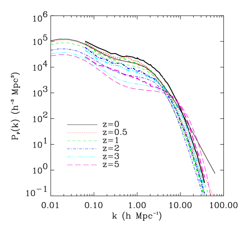
FIG. 4.: Power spectrum of the gas pressure at different redshifts. The thin smooth curves correspond to the analytical halo model (with $M_{\rm min}=5\times 10^{10}h^{-1}M_{\odot}$ and $M_{\rm max}=8\times 10^{14}h^{-1}M_{\odot}$), while the thick broken lines correspond to the simulations.

It is useful to consider the bias of the gas pressure relative to the dark matter density,

$$b_{p}^{2}(k,z)\equiv\frac{P_{p}(k,z)}{P(k,z)}.$$ (27)

It is shown for different redshifts on Figure 5.

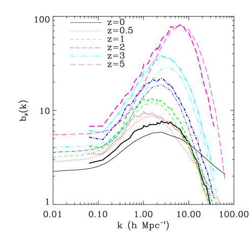
FIG. 5.: Bias $b_{p}(k)$ of the gas pressure with respect to the DM density (see text) at different redshifts. As before, predictions for both the halo model (with $M_{\rm min}=5\times 10^{10}h^{-1}M_{\odot}$ and $M_{\rm max}=8\times 10^{14}h^{-1}M_{\odot}$) and for the simulations are shown.

On large scales ($k\rightarrow 0$), the 2-halo term dominates and $P(k)\simeq P_{\rm lin}(k)$, so the pressure bias reduces to

$$b_{p}(k\rightarrow 0)\simeq\frac{1}{\overline{\rho}\overline{T}_{\rho}}\int_{M_{\rm min}}^{M_{\rm max}}dM~{}\frac{dn}{dM}b(M)MT.$$ (28)

In this limit, the pressure bias is thus simply the pressure-weighted average of the halo bias $b(M)$. The large scale pressure bias (at $k=0.06h$ Mpc^-1 derived from Eq [27]) is plotted in Figure 6 for different mass ranges ($M_{\rm min}$, $M_{\rm max}$).

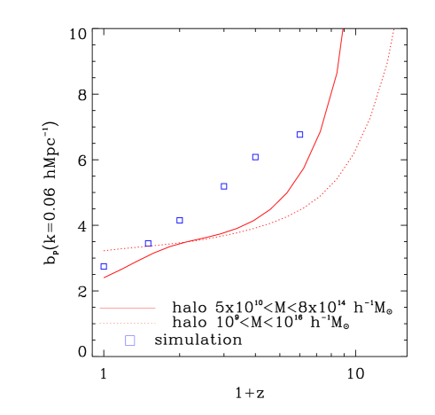
FIG. 6.: Large scale bias $b_{p}$ of the gas pressure as a function of redshift. The predictions from the halo model (for different mass ranges) and simulation are shown for $k=0.06h^{-1}$ Mpc.

IV Simulations

The halo model we described above relies on strong assumptions, namely that the mass density and pressure can be described statistically as a collection of spherically symmetric, isothermal halos in hydrostatic equilibrium. Although complicated structures, like walls and filaments, are known to exist in the hierarchical clustering picture, it remains to be established whether their influence on the resulting pressure power spectrum is sufficient to invalidate our simple halo model. In the following, we describe the high-resolution hydrodynamical simulations we have used to check the domain of validity of our analytical approach.

A Cosmological simulations using Adaptive Mesh Refinement

Adaptive Mesh Refinement (AMR) is now widely used in astrophysics [41, 42, 43, 44, 48] and offers an interesting alternative to the Smooth Particle Hydrodynamics (SPH) algorithm. AMR was recently adapted to the cosmological framework by several groups [42, 49]. The main advantage of this grid-based method, compared to the well-known Smooth Particle Hydrodynamics (SPH) method [46], is its ability to capture shock-waves and contact discontinuities using only a few resolution elements (typically 2-3 cells). In comparison, SPH demands at least 50 particles per resolution element, in order to minimize Poisson noise related to the discrete nature of the algorithm [47].

The basic AMR idea is to refine recursively an initially coarse grid (defined here as the coarse level $\ell=0$) with smaller and smaller cells of comoving size $\Delta x=2^{-\ell}$ ($\ell>0$). These refinements take place in regions where interesting features of the flow demand better spatial resolution (see Figure 8). For example, in fluid dynamics, one usually refines sharp discontinuities like shocks or contact surfaces. In cosmology, refinements are used within high-density regions, in order to resolve properly the gravitational collapse of small scale halos and the progressive build-up of large, massive ones. Due to the highly compressible nature of the self-gravitating cosmological fluid, this property improves dramatically the quality of the numerical solution.

In this paper, we use the results of a numerical simulation obtained using the newly developed RAMSES code, described in details in [23]. This code is based on general AMR techniques, with several specific properties that we briefly recall here. Contrary to patch-based AMR, where a small number of individual grids (say a few thousands) define rectangular regions of higher and higher resolution (see for example [42, 43, 48]), RAMSES is a cell-based AMR: each cell can be independently divided in sub-cells and thus can describe complex flow features of arbitrary geometry (see for example [49, 52]). The price to pay for this improved flexibility is a higher computational complexity: to describe the AMR grid, we use the “Fully Threaded Tree” data structure described by Khokhlov [52], where cells are placed in a recursive tree connecting each cell to its 8 sister cells and its 6 neighboring cells, with minimum memory overhead.

The N-body module of RAMSES is similar to the Adaptive Refinement Tree (ART code) of Kratsov, Klypin & Khokhlov [49], with some differences outlined in Teyssier [23]. The hydrodynamics module of RAMSES uses an unsplit, second-order Godunov scheme. Time integration proceeds in two different ways in RAMSES, either using a single, small time step for all levels of refinement or using nested, adaptive time steps in order to speed up the calculation for coarse levels. The last option was retained for cosmological simulations and turned out to speed up the calculation by a factor of 10, compared to the single-time step case. A complete presentation of the performances obtained by RAMSES is presented in Teyssier [23], using standard tests to validate our algorithm and its application to cosmological hydrodynamics.

B Simulation Parameters

In this paper, we present the results of a RAMSES simulation for a flat $\Lambda$CDM model with $\Omega_{M}=0.3$, $\Omega_{\Lambda}=0.7$, $\Omega_{B}=0.039$. We use the transfer function given in [54]. The resulting power spectrum is normalized to the COBE data [55] (this corresponds in our case to $\sigma_{8}=0.93$). The comoving box size was set to 100$h^{-1}$Mpc, imposing a maximum scale length in the simulation: $k_{min}=0.06$ $h$ Mpc^-1. Initial conditions are specified using an initial grid of $128^{3}$ dark matter particles. This corresponds to a mass resolution of $M_{\rm min}=4\times 10^{10}~{}M_{\odot}$. The particles were initially displaced according to the Zel’dovich approximation up to the starting redshift $z_{i}\simeq 55$. The baryon density and velocity fields were perturbed accordingly. We assume that baryons are described by a purely adiabatic, $\gamma=5/3$, fully ionized plasma. Since we are studying the SZ effect, we are mainly concerned by the pressure field of the baryons, which, at the scales of interest here, should remain unaffected (at least to first order) by neglecting others physical processes such as cooling, star formation and supernovae energy feedback. We plan to study the influence of these others physical inputs in a future paper.

The key parameters of any AMR simulation are the refinement criteria used to dynamically create the refinement tree. We use the “quasi-Lagrangian” approach described in Kratsov, Klypin & Khokhlov [49]. The idea is to mark for refinement any cells whose gas or dark matter overdensity exceeds a level-dependent threshold given by

$$\frac{\rho}{\bar{\rho}}(\ell=0,5)=1,80,640,5120,20480,163840$$ (29)

The coarse grid ($\ell=0$) is nothing but the $128^{3}$ particle grid used to set up the initial conditions. The $\ell=0$ refinement criteria ($\rho/{\bar{\rho}}>1$) ensures that, initially, the whole computational volume is covered by a $256^{3}$ grid ($\ell=1$). In this way, initial small scale perturbations are sampled by two grid points, which turns out to be necessary to avoid small scale power damping. At later times, large voids appear in the simulation where the resolution is locally degraded down to the $128^{3}$ coarse grid. For higher levels of refinements, the density thresholds are chosen in order to refine cells that contains between 5-10 particles (or fluid mass elements). This “quasi-Lagrangian” approach preserves the initial resolution in physical coordinates, adapting the local comoving spatial resolution to collapsing mass elements (see [45] for a complete discussion).

The maximum level of refinement reached at the end of the present run is $\ell=6$, which gives a formal spatial resolution of $8192^{3}$ (or 12 kpc $h^{-1}$ comoving) at $z=0$. The comoving spatial resolution scales roughly with redshift as $(1+z)^{-1}$. We also use the adaptive time-stepping procedure of RAMSES to speed up the computation: 157 time steps only were necessary at the coarse level while 8185 time steps were necessary at the finest level. The Layzer-Irvine energy conservation was better than $1\%$ at the end of the simulation. Starting with $19\times 10^{6}$ cells at $z_{i}=55$, we end up with $28\times 10^{6}$ cells at $z=0$ in the tree structure (including the coarse level). Six different output times were considered: $z=0,0.5,1,2,3$ and $5$.

C Effect of finite mass resolution and box size

The question that arises when interpreting numerical simulations is that of its range of validity. Here, we discuss three limitations of cosmological simulations which can introduce spurious effects: the finite box size, the mass resolution and the spatial resolution.

Since we solve for the gravitational evolution of the system assuming periodic boundary conditions, the power on scales larger than the box size is completely suppressed. This translates into a maximum mass above which no halo can form. Indeed, the probability to find a large halo of mass, say, $10^{16}h^{-1}M_{\odot}$ in our computational box is close to zero. An estimate for the maximum mass $M_{\rm max}$ which corresponds to our box size is given by

$$n(>M_{\rm max})L_{\rm box}^{3}=1$$ (30)

where $n(>M)$ is the cumulative Press-Schechter mass function. For $L_{\rm box}$ = 100 $h^{-1}$Mpc, this gives $M_{\rm max}\simeq 7\times 10^{14}h^{-1}M_{\odot}$. Note that, on large scales, we are dominated by the “cosmic variance” of the simulation: depending on the exact random field realization for the initial conditions, we may still form by chance a very large cluster in the simulation. The next step is to check the convergence of various quantities with respect to $M_{\rm max}$, using our analytical model. As we show below (§V E), we find that good convergence in the SZ power spectrum is achieved for $M_{\rm max}=2\times 10^{15}h^{-1}M_{\odot}$, or equivalently $L_{\rm box}$ = 400 $h^{-1}$Mpc. On the other hand, for a fixed number of particles, increasing the box size inevitably degrades the mass and spatial resolutions of the simulation. Our current choice of $L_{\rm box}$ = 100 $h^{-1}$Mpc is a trade off between these two opposite constraints.

The mass resolution, $M_{\rm min}\propto k_{\rm max}^{-3}$, is related to the small scale power in the initial conditions. No object with $M\leq M_{\rm min}$ will form, leaving instead a cold, smooth background between collapsing objects. In order to account for these two effects (finite box size and mass resolution), we introduced in the analytical description a mass range where the different integrals are computed. This limited mass range is supposed to mimic the lack of large mass haloes due to the finite box size ($M_{\rm max}$), and the lack of small mass halos due to the power cut off at small scale ($M_{\rm min}$).

The final numerical effect which needs to be examined is the spatial resolution. The spatial resolution is related to the minimum scale below which the code is not able to solve the equations. For example, in a standard Particle Mesh code, this scale is equal to 2 cell size of the underlying Cartesian mesh, below which the force between 2 interacting particles goes smoothly to zero. In practice, this acceleration cut off at small radii results in a damping of the power spectrum up to scales as large as 8 comoving cell size. For gas dynamics, the problem of spatial resolution is even more crucial. Shock waves need at least 2 cells to be properly resolved. If small scale velocity fluctuations are not properly sampled, no shock dissipation can occur at all. In this case, the small scale density fluctuations are only compressed adiabatically, i.e. they remain cold, even though their temperature should rise to the virial temperature. This can affect both the mean and the variance of the computed gas pressure.

During the course of gravitational collapse, the initial perturbations contract at smaller and smaller comoving scales, making the spatial resolution issue even more crucial. The spatial resolution therefore translates directly into a minimum mass, below which halo collapse cannot be resolved properly by the code. For a Particle-Mesh code, coupled to a standard gas dynamics code, the resulting minimum mass can be as high as 100 particles, for a halo to be properly resolved. Most of the initial small scale power is then lost this way. As discussed in section §IV A, AMR techniques allows one to dynamically adapt the comoving resolution to the collapsing mass element. In light of the results obtained in this paper, we claim that the RAMSES code allows us to resolve properly small scale shock heating, down to the minimal halo mass imposed by the initial conditions.

D Computation of the Power spectrum

In this paper, we need to compute the DM density power spectrum, together with that of the gas pressure. Since the spatial resolution goes from 96 kpc $h^{-1}$ at $z=5$ down to 12 kpc $h^{-1}$ at $z=0$ for a box size of 100 Mpc $h^{-1}$, the dynamical range imposes a severe challenge in computing power spectra. The brute force approach would consist in Fourier analyzing each field on a large Cartesian grid of $1024^{3}$ for $z=5$ (barely feasible on a supercomputer), up to a Cartesian grid of $8192^{3}$ for $z=0$ (completely out of reach).

A more appropriate approach is described in Jenkins et al. [51] and Kravtsov & Kylpin [50]. The idea is to define each field (dark matter density or gas pressure) in a nested structure of tractable mesh (we use $128^{3}$ cells). At each level $\ell$, we divide the whole computational volume in $\ell^{3}$ Cartesian $128^{3}$ sub-cubes and add up the fields computed in all these sub-cubes together. We then use a standard Fourier power spectrum estimation for the resulting field. Each scale $\ell$ provides a reliable power spectrum estimation between $2^{\ell}\times[k_{\rm min},k_{\rm max}]$, where $k_{\rm min}\approx 8(2\pi/L_{\rm box})$ and $k_{\rm max}\approx 16(2\pi/L_{\rm box})$. These limits are determined empirically, by comparing the results obtained for 3 nested $128^{3}$ grids and for a single $512^{3}$ grid. The resulting power spectrum estimation is obtained by combining the different “band power” estimates together. Finally, we subtract from the dark matter density power spectrum the shot noise (or Poisson noise) due to the discrete nature of the particle distribution.

V Results

A Dark Matter Power Spectrum

Figure 1 shows the dark matter power spectrum $P(k)$ at different redshifts, derived from the Peacock & Dodds [38] formalism, the halo method and the simulations. The finite box size and the mass resolution (see the Poisson noise limit on the figure) restricts predictions of the simulations to the range $0.06\lesssim k\lesssim 60$ $h$ Mpc^-1. For all redshifts, the simulations agree very well with Peacock & Dodds within this range, which spans 3 orders of magnitude. This range is consistent with the formal spatial resolution of the simulation, which spans 4 order of magnitude, after accounting for the small scale power damping discussed in §IV C. In comparison, the simulations used by Refregier et al. [19] and Seljak, Burwell, & Pen [20] agreed with Peacock & Dodds only within one order of magnitude in $k$, and therefore seriously limited the SZ predictions of these authors [19]. The present simulations therefore allow us to significantly improve over these previous works.

As stated in §III A, the halo model prediction for $P(k)$ is in good agreement with the Peacock & Dodds spectrum for all redshifts (see [32]). Small deviations of the order of a few percents can be noticed for $k\lesssim 10$ $h$ Mpc^-1, but are acceptable for our purposes. Note in particular that the evolution of the break in the power spectrum between the linear and the nonlinear regime is well modeled by the halo model.

B Temperature Evolution

Figure 2 shows the evolution of the mass-weighted temperature $\overline{T}_{\rho}(z)$ (Eq. [2]) as predicted from the halo model (Eq. [18]) and from the simulation. For the halo model, different mass cut off ranges $M_{\rm min}<M<M_{\rm max}$ (see Eq. [18]) are examined.

The halo prediction is sensitive to $M_{\rm max}$ and $M_{\rm min}$ at low and high redshift, respectively. At high redshift, the characteristic non-linear mass scale $M_{\star}$ is close to the mass resolution of the simulation, for which no shock heating can occur. Logically, this translates in an underestimation of the mean temperature. At low redshift, the non-linear mass scale $M_{\star}$ approaches dangerously the maximum mass scale due to the finite box size. Here again, the temperature is underestimated, but this time, it is due to the absence of very high mass halos.

A good overall agreement (mean temperature and power spectrum evolution) between the simulation and the analytical model is obtained for the following mass range:

$$5\times 10^{10}<M<8\times 10^{14}h^{-1}M_{\odot}$$ (31)

It is reassuring that this best-match mass limits are close to the natural limits imposed by the simulation, as shown in §IV C.

For a mass range of $5\times 10^{10}<M<4\times 10^{14}h^{-1}M_{\odot}$, the mean temperature evolution for the halo model (not shown on Figure 2) is virtually indistinguishable from the simulation curve, with $\overline{T}(z=0)\simeq 0.34$ and 0.33 keV, respectively. However, as we will see below (§V E), the agreement with the pressure power spectrum slightly worsens. For $M_{\rm max}=8\times 10^{14}$ (our fiducial limit) and $M_{\rm max}>10^{16}$ $h^{-1}M_{\odot}$ (the converged asymptotic limit) the halo model predicts $\overline{T}(z=0)\simeq$ 0.41 and 0.50 keV, respectively.

C Mean Comptonization Parameter

Our calculation of the evolution of the density-weighted temperature allows us to compute the mean comptonization parameter (see Eq. [1]). For the simulation, we find $\overline{y}=2.65\times 10^{-6}$. The halo model with our fiducial mass limits (Eq. [31]) predicts a value of $\overline{y}=2.84\times 10^{-6}$. As expected, the agreement is slightly better for $M_{\rm max}\simeq 4\times 10^{14}h^{-1}M_{\odot}$ with $\overline{y}=2.72\times 10^{-6}$. In all cases, these values are similar to those found in other studies (eg. [14, 19, 29]). It is interesting to study how our prediction for $\overline{y}$ depends on the mass limits. We find experimentally that

$$\overline{y}\simeq 2.84\times 10^{-6}\left(\frac{M_{\rm min}}{5\times 10^{10}h^{-1}M_{\odot}}\right)^{-0.06}\left(\frac{M_{\rm max}}{8\times 10^{14}h^{-1}M_{\odot}}\right)^{0.01}.$$ (32)

Since length scales scale as $M^{\frac{1}{3}}$, this means that $\overline{y}\propto\Delta^{-0.2}L^{0.03}$, where $\Delta$ is the effective resolution length and $L$ is the box size of the simulation. This quantity is thus quite sensitive to the mass resolution, but not very sensitive to the box size. This should be kept in mind when interpreting and comparing the predictions of simulations. The asymptotic value corresponding, effectively, to an infinite mass range is $\overline{y}\simeq 3.01\times 10^{-6}$ (for $z_{i}=10$, see II).

D Projected Map of the Pressure

Figure 7 shows a map of the $y$-parameter projected through one side of the $100h^{-1}$ Mpc box at $z=0$. Clusters produces fluctuations in $y$ of the order of $10^{-4}$–$10^{-6}$, while supercluster filaments produce fluctuations of the order of $10^{-6}$–$10^{-8}$ . This figure is quite similar to the corresponding figure from Refregier et al. [19] derived from the Moving Mesh Hydrodynamical code (MMH) of Pen [17, 18]. Note however, the more circular appearance of clusters in our simulations, compared to the more elongated cores seen in that of Refregier et al. [19]. The number of small mass objects is also much higher in our simulation. The main difference between RAMSES and MMH is the spatial resolution. The improved dynamical range of RAMSES compared to MMH yields to the fragmentation of large scale filements into small clumps. The effective mass resolution in RAMSES is consequently much smaller than the one reached with MMH. Moreover, substructures within large halos, clearly visible in Figure 7, are able to survive to tidal stripping much longer in RAMSES than in MMH. This explains the more elongated cores of large halos in MMH simulations.

FIG. 7.: Map of the $y$-parameter projected through on face of the $100h^{-1}$ Mpc box at $z=0$.

Figure 8 shows a close up of one the clusters in the AMR simulation. Panel (a) shows the map of the $y$-parameter for the cluster, while the panel (b) shows the AMR grid for this region. Notice how the AMR grid has adapted to provide higher resolution for the cluster core and for the two substructures below the cluster. The virial radius for this cluster is about $1$-$1.5h^{-1}$ Mpc, and thus almost entirely fills the displayed region ($3.12h^{-1}$ Mpc on a side). This figure also shows that the structure of individual clusters is more complicated than that assumed in our halo model. In the following, we show that the halo model nevertheless provides an acceptable prediction for the pressure power spectrum.

E Pressure Power Spectrum

Figure 4 shows the power spectrum of the gas pressure at different redshifts for both the fiducial halo model (with our fiducial mass range of Eq. [31]) and for the simulations. The overall agreement is remarkable: the shape of the power spectra agree approximately for both methods, along with the scaling with redshifts which changes order above and below $k\sim 3h^{-1}$ Mpc^-1. According to both method, the pressure power spectrum does not evolve as much as the DM density power spectrum. Qualitatively, this is due to the fact that, at large redshift the smaller amplitude of the density power spectrum is compensated by the larger biasing of peaks with high temperature which dominate the pressure power spectrum.

There are nevertheless quantitative differences: the halo model predictions have somewhat different normalization at low $k$ and not exactly the same shape at large $k$. This can be seen more clearly by studying Figure 5, which shows the bias $b_{p}(k)$ of the gas pressure (Eq. [27]) at different redshifts. Again both the simulation and fiducial halo model are displayed. Note that we used the halo-model power spectrum in the denominator in both cases, so that Figure 5 is nothing but a change of scaling of the pressure power spectrum.

FIG. 8.: Close up on a cluster in the simulation. (a) Map of the $y$-parameter for the cluster. The logarithmic color scale ranges from $y=10^{-7}$ to $10^{-4}$. The image size is $3.12h^{-1}$Mpc on a side. (b) AMR grid for this region with levels from $\ell=1$ to 6.

The difference in shape at large $k$ is more pronounced at low redshifts where the simulation pressure spectrum falls off faster than the halo model. The shape of the pressure power spectrum at intermediate and small scales is determined by the interplay between the different characteristic radii $r_{v}$, $r_{s}$ and $r_{g}$ (see §III C). Figure 3 shows that at low redshifts the gas inner radius $r_{g}$ is smaller at the relevant mass ($M_{*}$ is about $10^{14}h^{-1}M_{\odot}$) and is dangerously close to the effective resolution limit (about $12h^{-1}$ kpc) of the simulation. This would tend to reduce the pressure power at small scale in the simulation and thus explain the discrepancy. Numerical dissipation could also be at the origin of this small scale power damping (at a scale comparable to the spatial resolution). Indeed, this effect tends to induce a spurious increase in entropy, which results in a larger “core radius” in the gas distribution. Finally, the disagreement could also be caused by the limitations of the halo model. As Figure 8 illustrates, the structure of clusters is more complicated than that assumed in our model. In particular, cluster profiles may not be isothermal. In fact, our simulations indicate that the gas temperature tends to rise towards the center of clusters. This would lead to larger effective core radii and thus tend to suppress power on small scales. This effect could thus explain the discrepancy, as it is more pronounced at low redshifts.

The mismatch of the normalization at small $k$ can be studied using Figure 6, which shows the large-scale pressure bias as a function of redshift for both methods. The squares show the predictions for the simulations at the largest available scale, $k=0.06h$ Mpc^-1. The solid line shows the fiducial halo prediction at the same scale (derived from Eq. [27]). Both methods predict that the pressure bias increases with redshift, and agree relatively well for $z\lesssim 1$. The two methods however disagree by about 40% at $z\simeq 3$. In addition, the change of slope predicted by the halo model at this redshift is not observed in the simulations.

The large scale pressure bias depends on the mass range chosen for the halo model. This can be seen by examining the dotted curve in Figure 6. It shows the halo prediction for a wide mass range, which has reached convergence to the asymptotic limit of an infinite mass range. This curve and that corresponding to the fiducial mass range agree at intermediate redshifts ($1\lesssim z\lesssim 2$), but differ both at lower and higher redshifts: increasing $M_{\rm max}$ tends to increase $b_{p}$ at low redshift, while decreasing $M_{\rm min}$ tends to decrease $b_{p}$ at large redshift. While this dependence must be taken into account, we could not find any reasonable mass range which eliminated the discrepancy with the simulations.

The halo prediction for the asymptotic case of $k\rightarrow 0$ (Eq. [28]) differs from the $k=0.06h^{-1}$ Mpc curves shown in Figure 6, only by about 20%. It therefore captures the dominating dependence of the large-scale pressure bias, and can thus be used to understand the origin of the discrepancy. For a given choice of the mass range, the asymptotic halo prediction is very robust. Indeed, once the mass function has been fixed to ensure an agreement with the DM density power spectrum, $b_{p}(0)$ only depends on the halo bias function $b(\nu)$. After experimenting, we found that a modification of the Mo & White [37] relation for $b(\nu)$ (Eq. [11]) can indeed reduce the discrepancy. This is however poorly motivated, and would not be necessarily consistent with the observed clustering of DM haloes in N-body simulations [37, 56, 57, 58, 59]. The Sheth, Mo & Tormen [57] $b(\nu)$ relation was shown to better agree with N-body results [59]; its use in place of the Mo & White relation however slightly worsens the discrepancy for the gas pressure. We therefore do not pursue this possibility here.

Instead, we note that this discrepancy for the large-sale pressure bias could come from the limitations of the halo model. It indeed assumes that that all the matter can be modeled as a collection of collapsed halo. At early times and on large scales, filaments and sheets indeed dominate the large-scale structure and are awkwardly described by the halo model. Visual inspection of SZ maps obtained by the simulation at large redshifts ($z=2$-$3$) confirms this tendency qualitatively.

Our results for the pressure bias are in good qualitative agreement with Figure 6 in Refregier et al. [19]. They however find a faster fall off at large $k$ and a larger evolution of the pressure bias $b_{p}(k)$. These two facts can be explained by the coarser spatial resolution of their simulations, which, as discussed in §IV C, translates into a larger effective mass resolution ($M_{\rm min}\simeq 5\times 10^{12}h^{-1}M_{\odot}$).

F Sunyaev-Zel’dovich Power Spectrum

From the estimates of the evolution of the pressure power spectrum and of the density-weighted temperature, we can compute the SZ power spectrum, using Equation (3). The resulting spectra are shown in Figure 9 for the simulations, the halo model with our fiducial mass range, and the asymptotic halo model. The primordial CMB power spectrum for our $\Lambda$CDM model is also shown, as derived using CMBFAST [60].

The agreement between our fiducial halo model (dashed line) and the simulations (dotted line) is excellent, showing that some of the discrepancies in the pressure power spectrum cancel out when integrated along the line of sight.

The dot dashed line in Figure 9 shows the halo prediction for a wide mass range (corresponding to a good approximation to the asymptotic limit $0<M<\infty$). This model agrees with our fiducial model (and the simulations) for $\ell\gtrsim 7000$, but exceeds it by a factor of as much as $\sim 2$ below that. Note that the difference comes primarily from the larger $M_{\rm max}$ value, while a change in $M_{\min}$ has very little effect. This shows that the main limitation of the simulation is the finite box size, which limits the number of massive clusters at low redshifts.

The impact of spatial resolution can be studied by examining Figure 10. For this figure, the SZ power spectrum was computed from the fiducial halo model, after restricting the integration of the pressure power spectrum to different upper bounds $k_{\rm max}$ for the wavenumber $k$. (In all cases, the minimum bound was chosen to be $k_{\rm min}=0.06h$ Mpc^-1, the value imposed by the finite size of the simulation box). The figure shows that the SZ power spectrum is quite sensitive to the spatial resolution (i.e. to $k_{\rm max}$). A degradation of the spatial resolution to $k_{\rm max}\simeq 5h$ Mpc^-1 leads to a severe drop of power for $\ell\gtrsim 2\times 10^{3}$ (see also [19]). Interestingly, the SZ spectrum does not vary much if $k_{\rm max}$ is taken be 20 $h$ Mpc^-1 or above. For our simulation, $k_{\rm max}\simeq 60h$ Mpc^-1 at low redshifts, which is sufficient to reach convergence. The main limitation of our prediction from the simulation is thus that arising from the finite box size. On the other hand, thanks to the AMR scheme, spatial and mass resolution are not a limiting factor.

Our prediction for the SZ power spectrum agrees approximately with the results of da Silva et al. [15], up to a small overall rescaling due to our larger value of $\sigma_{8}$. Our results also agree with the prediction of Refregier et al. [19], within their $\ell$-range of confidence. As they noted, their predictions were limited by the spatial resolution of their simulations, which corresponds to $k_{\rm max}\approx 5h$ Mpc^-1. Our curve in Figure 10 corresponds to this value of $k_{\rm max}$ and is in good agreement with their result.

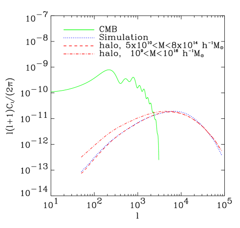
FIG. 9.: SZ power spectrum for the halo model and for the simulations, in the RJ regime. The spectrum for the halo model is shown for different mass ranges: our fiducial mass range (dashed) and the asymptotic halo model (dot-dashed). The primordial CMB power spectrum for the $\Lambda CDM$ model is also shown for comparison.

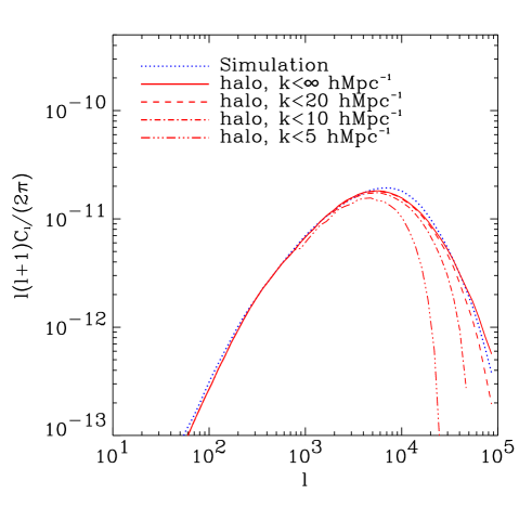
FIG. 10.: SZ power spectrum for the halo model with different values of $k_{\max}$. Our fiducial mass limits of $M_{\rm min}=5\times 10^{10}h^{-1}M_{\odot}$ and $M_{\rm max}=8\times 10^{14}h^{-1}M_{\odot}$, and a value of $k_{\min}=0.06h$ Mpc^-1 were adopted. The power spectrum of the simulations is also shown for comparison.

VI Conclusions

We have studied the 2-point statistics of the gas pressure and of the resulting SZ fluctuations using two methods: a RAMSES numerical simulation, using Adaptive Mesh Refinement, and an analytical halo model. Overall, the agreement is good, once the mass resolution and finite box size of the simulations are accounted for. The agreement is almost surprising, given the simple nature of the halo model. The halo model[21] is self-consistent and relies on the assumption of virial and hydrostatic equilibrium of the gas. After it has been tuned to produce the correct DM density power spectrum, the model does not require any new free parameters and thus has a strong predictive power.

The predictions for the SZ power spectrum from our numerical simulations are mainly and solely limited by the finite box size. The AMR techniques indeed gives a reliable dynamic range of about 3 orders of magnitude for the power spectra, corresponding to a formal resolution of 8192 in linear scale, relieving us from the limiting effect of finite spatial resolution. The halo model allows us to extrapolate to an infinite box size, thus providing us with an accurate SZ power spectrum in the full multipole range $10^{2}\lesssim\ell\lesssim 10^{5}$. This is an important improvement upon earlier calculations [19, 20] which were severely affected for $\ell\gtrsim 2\times 10^{3}$ by their coarser spatial resolution.

In principle, the effect of finite box size could be alleviated using larger simulations, as discussed in §IV C. However, to achieve convergence, one would need to reach a limiting mass of $M_{\rm max}=2\times 10^{15}h^{-1}M_{\odot}h^{-1}$ which would correspond to a box size of 400 $h^{-1}$ Mpc in a $\Lambda$CDM model. Given our current computer resources, this is prohibitive for the near future. One thus has to rely, as we have done, on analytical models to extrapolate beyond the sampling variance of the simulations. Analytical models, like the one we have presented here, also have the advantage of providing a fast way to explore a wide range of cosmological parameters. They also help to provide a physical understanding of the physics and scales which contribute to the SZ statistics. Using our halo model, we have shown for example that two characteristics length scales contributes to the SZ power spectrum: the virial radius $r_{v}$ and the gas inner radius $r_{g}$. It would be interesting to understand in more details how the SZ power spectrum provides a measure of the different regions of the NFW profile on a range of mass scales. Another interesting avenue is the study of processes such as feedback and cooling on the SZ statistics. This will be explored in future work.

- [1] R. A. Sunyaev and Ya. B. Zel’dovich, Ya.B., Comm. Astrophys. Space Phys. 4, 173 (1972).
- [2] R. A. Sunyaev and Ya. B. Zel’dovich, Ann. Rev. Astron. Astrophys. 18, 357 (1980).
- [3] Y. Rephaeli, Ann. Rev. Astron. Astrophys. 33, 541 (1995).
- [4] M. Birkinshaw, Phys. Rept. 310, 97 (1999).
- [5] A. Refregier, Invited review in Microwave Foregrounds, eds A. de Oliveira-Costa and M. Tegmark, (ASP: San Francisco, 1999).
- [6] J. E. Carlstrom, M. K. Joy, L. Grego, G. P. Holder, W. L. Holzapfel, J. J. Mohr, S. Patel and E. D. Reese, in Nobel Symposium Particle Physics and the Universe”, to appear in Physica Scripta and World Scientific, eds. L. Bergstrom, P. Carlson and C. Fransson, preprint astro-ph/9905255.
- [7] K. Grainge, M. E. Jones, G. Pooley, R. Saunders, A. Edge and R. Kneissl, Mon. Not. R. Astron. Soc. (submitted), preprint astro-ph/9904165.
- [8] N. Aghanim, A. De Luca, F.R. Bouchet, R. Gispert, & J.L. Puget, AStron. AStrophys., 325, 9 (1997)
- [9] A. Refregier, D.N. Spergel, & T. Herbig, /apj, 531, 79 (2000)
- [10] A. Cooray, W. Hu, & M. Tegmark, submitted to ApJ, preprint astro-ph/0002238 (2000)
- [11] F. Atrio-Barandela and J. P. Mücket, ApJ515, 465 (1999).
- [12] E. Komatsu and T. Kitayama, ApJLett. 526, L1 (1999) [KK99].
- [13] R. Scaramella, R. Cen and J. P. Ostriker, ApJ416, 399 (1993).
- [14] A. da Silva, D. Barbosa, D., A. R. Liddle and P. A. Thomas, Mon. Not. R. Astron. Soc. (submitted), astro-ph/9907224.
- [15] A. da Silva, D. Barbosa, D., A. R. Liddle and P. A. Thomas, Mon. Not. R. Astron. Soc. (submitted), astro-ph/0011187.
- [16] F. M. Persi, D. N. Spergel, R. Cen and J. P. Ostriker, ApJ442, 1 (1995).
- [17] U. Pen, ApJSuppl. 100, 269 (1995).
- [18] U. Pen, ApJSuppl. 115, 19 (1998).
- [19] A. Refregier, E. Komatsu, D.N. Spergel, & U.-L. Pen, Phys. Rev. D, 61, 123001 (2000)
- [20] U. Seljak, B. Juan and U. Pen, submitted to Phys. Rev. D, preprint astro-ph/0001120 (2000)
- [21] A. Cooray, Phys. Rev. D 62, 103506 (2000)
- [22] P. Zhang & U.-L. Pen, submitted to ApJ, preprint astro-ph/0007462 (2000)
- [23] R. Teyssier, 2001, in preparation
- [24] D. N, Schramm and M. S. Turner, Rev. Mod. Phys. 70, 303 (1998).
- [25] A. Stebbins, lectures at NATO ASI “The Cosmic Microwave Background” Strasbourg 1996, preprint astro-ph/9705178 (1997).
- [26] D. J. Fixsen, E. S. Cheng, J. M. Gales, J. C. Mather, R. A. Shafer and E. L. Wright, ApJ473, 576 (1996).
- [27] N. Kaiser, ApJ498, 26 (1998).
- [28] N. Y. Gnedin, ApJ, 535, 530 (2000).
- [29] U. Seljak, Mon. Not. R. Astron. Soc. 318, 203 (2000)
- [30] C.-P. Ma & J.N. Fry, to appear in ApJ544, preprint astro-ph/0003343 (2000)
- [31] J.M. Bardeen, J.R. Bond, N. Kaiser, & A.S. Szalay ApJ, 304, 15 (1986)
- [32] A. Cooray, W. Hu & J. Miralda-Éscude, ApJ535, L9 (2000)
- [33] J. A. Peacock, Mon. Not. R. Astron. Soc. 284, 885 (1997)
- [34] T. Kitayama and Suto Y. ApJ469, 480 (1996)
- [35] W. H. Press and P. Schechter, Astrophys. J. 187, 425 (1994).
- [36] J.J. Navarro, C.S. Frenk, & S.D.M. White, ApJ, 462, 563 (1996)
- [37] H.J. Mo & S.D.M. White Mon. Not. R. Astron. Soc. 282, 347 (1996)
- [38] J. A. Peacock and S. J. Dodds, Mon. Not. R. Astron. Soc. 280, L19 (1996).
- [39] V.R. Eke, S. Cole, & C.S. Frenk, Mon. Not. R. Astron. Soc. 282, 263 (1996)
- [40] G. L. Bryan and M. L. Norman, ApJ495, 80 (1998).
- [41] R. I. Klein, C. F. McKee, C. F. & P. Colella, 1994, ApJ, 420, 213
- [42] G. L. Bryan & M. L. Norman, 1997, ASP Conf. Ser. 123: Computational Astrophysics; 12th Kingston Meeting on Theoretical Astrophysics, 363
- [43] J. K. Truelove, R. I. Klein, C. F. McKee, J. H. II Holliman, L. H. Howell, J. A. Greenough, D. T. Woods ApJ495, 821 (1998)
- [44] A. M. Khokhlov, P. A. H flich, E. S. Oran, J. C. Wheeler, L. Wang, and A. Yu. Chtchelkanova, ApJ524, L107 (1999)
- [45] A. Knebe, A. V. Kravtsov, S. Gottlöber & A. A. Klypin, 2000, MNRAS, 317, 630
- [46] J. J. Monaghan, 1992, ARA&A, 30, 543
- [47] H. Kang, J. P. Ostriker, R. Cen, D. Ryu, L. Hernquist, A. E. Evrard, G. L. Bryan & M. L. Norman, 1994, ApJ, 430, 83
- [48] P. M. Ricker, et al. 1999, American Astronomical Society Meeting, 195, 4205
- [49] A. V. Kravtsov, A. A. Klypin, & A. M. Khokhlov, 1997, ApJS, 111, 73
- [50] A. V. Kravtsov, & A. A. Klypin, 1999, ApJ, 520, 437
- [51] A. Jenkins, et al. 1998, ApJ, 499, 20
- [52] A.M. Khokhlov, 1998, J. Comput. Phys, 143, 519
- [53] C. S. Frenk, et al. 1999, ApJ, 525, 554
- [54] Ma, C. 1998, ApJL, 508, L5
- [55] M. White, & E. F. Bunn, 1995, ApJ, 450, 477
- [56] R.K. Sheth & G. Tormen, Mon. Not. R. Astron. Soc. 308, 119 (1999)
- [57] R.K. Sheth, H.J. Mo, & G. Tormen, submitted to Mon. Not. R. Astron. Soc., preprint astro-ph/9907024 (1999)
- [58] Y. Jing, ApJ503, L9 (1998)
- [59] J. Robinson, submitted to Mon. Not. R. Astron. Soc., preprint astro-ph/0004023 (2000)
- [60] M. Zaldarriaga & U. Seljak, ApJSupplement, in press, preprintastro-ph/9912199 (1999)