The Luminosity Function of Galaxies in SDSS Commissioning Data¹

Abstract

In the course of its commissioning observations, the Sloan Digital Sky Survey (SDSS) has produced one of the largest redshift samples of galaxies selected from CCD images. Using 11,275 galaxies complete to $r^{\ast}=17.6$ over 140 square degrees, we compute the luminosity function of galaxies in the $r^{\ast}$ band over a range $-23<M_{r^{\ast}}<-16$ (for $h=1$). The result is well-described by a Schechter function with parameters $\phi_{\ast}=(1.46\pm 0.12)\times 10^{-2}$ $h^{3}$ Mpc^-3, $M_{\ast}=-20.83\pm 0.03$, and $\alpha=-1.20\pm 0.03$. The implied luminosity density in $r^{\ast}$ is $j\approx(2.6\pm 0.3)\times 10^{8}hL_{\odot}$Mpc^-3. We find that the surface brightness selection threshold has a negligible impact for $M_{r^{\ast}}<-18$. Using subsets of the data, we measure the luminosity function in the $u^{\ast}$, $g^{\ast}$, $i^{\ast}$, and $z^{\ast}$ bands as well; the slope at low luminosities ranges from $\alpha=-1.35$ to $\alpha=-1.2$. We measure the bivariate distribution of $r^{\ast}$ luminosity with half-light surface brightness, intrinsic $g^{\ast}-r^{\ast}$ color, and morphology. In agreement with previous studies, we find that high surface brightness, red, highly concentrated galaxies are on average more luminous than low surface brightness, blue, less concentrated galaxies. An important feature of the SDSS luminosity function is the use of Petrosian magnitudes, which measure a constant fraction of a galaxy’s total light regardless of the amplitude of its surface brightness profile. If we synthesize results for $R_{\mathrm{GKC}}$-band or $b_{j}$-band using these Petrosian magnitudes, we obtain luminosity densities 2 times that found by the Las Campanas Redshift Survey in $R_{\mathrm{GKC}}$ and 1.4 times that found by the Two-degree Field Galaxy Redshift Survey in $b_{j}$. However, we are able to reproduce the luminosity functions obtained by these surveys if we also mimic their isophotal limits for defining galaxy magnitudes, which are shallower and more redshift dependent than the Petrosian magnitudes used by the SDSS.

1 Motivation

A fundamental characteristic of the galaxy population, which has been the subject of study at least since Hubble (1936), is the distribution of their luminosities. Given the broad spectral energy distributions of galaxies (especially in the presence of dust), the bolometric luminosity of galaxies is currently too difficult to measure to meaningfully study, so we must be satisfied with observing the luminosity function in some wavelength bandpass. In this paper we measure the luminosity function of local ($z<0.2$) galaxies in five optical bandpasses, between about 3000 Å and 10000 Å. We also investigate the correlation of luminosity with other galaxy properties, such as surface brightness, intrinsic color, and morphology. This quantitative characterization of the local galaxy population provides the basic data that a theory of galaxy formation must account for and an essential baseline for studies of galaxy evolution at higher redshifts.

The most recent determinations of the optical luminosity function of “field” galaxies (those selected without regard to local density) have come from large flux-limited redshift surveys. They include the luminosity function measurements of Lin et al. (1996), using the Las Campanas Redshift Survey (LCRS; Shectman et al. 1996) in the LCRS $R_{\mathrm{GKC}}$-band (around 6500 Å), and of Folkes et al. (1999) using the Two-degree Field Galaxy Redshift Survey (2dFGRS; Colless 1999) in the $b_{j}$-band (around 4500 Å). Other recent determinations of the local optical luminosity function have been mostly in the $B$- or $b_{j}$-bands, for example the Nearby Optical Galaxy sample (Marinoni et al. 1999), the Optical Redshift Survey (Santiago et al. 1996), the Stromlo-APM Redshift Survey (Loveday et al. 1992), the Durham/UKST Galaxy Redshift survey (Ratcliffe et al. 1998), and the ESO Slice Project Galaxy Redshift Survey (Zucca et al. 1997). Of particular interest here is the ability to use the multi-band photometry of the SDSS to meaningfully compare our results to those of these other surveys.

In this paper, we use imaging and spectroscopy of 11,275 galaxies over about 140 square degrees complete to $r^{\ast}=17.6$ from the Sloan Digital Sky Survey (SDSS; York et al. 2000) commissioning data to calculate the luminosity function of galaxies. In Section 2 we describe the source catalog and the redshift sample, with particular attention to our definition of galaxy magnitudes, which is based on a modified form of the Petrosian (1976) system. In Section 3, we describe the maximum-likelihood method used to calculate the luminosity function. In Section 4, we present the results for the luminosity function in each band, for the luminosity density of the universe, and for the dependence of galaxy luminosity on surface brightness, color and morphology. In Section 5, we examine the effects of using Petrosian magnitudes rather than isophotal magnitudes for the luminosity function. In Section 6, we compare our results to those of Lin et al. (1996; LCRS) and Folkes et al. (1999; 2dFGRS). We show that the SDSS luminosity function implies a substantially higher mean luminosity density than either of these previous measurements, but that we can reproduce the results of both surveys if we mimic their isophotal definitions of galaxy magnitudes. We conclude in Section 7.

2 SDSS Commissioning Data

2.1 Description of the Survey

The SDSS (York et al. 2000) will produce imaging and spectroscopic surveys over $\pi$ steradians in the Northern Galactic Cap. A dedicated 2.5m telescope (Siegmund et al., in preparation) at Apache Point Observatory, Sunspot, New Mexico, will image the sky in five bands ($u^{\prime}$, $g^{\prime}$, $r^{\prime}$, $i^{\prime}$, $z^{\prime}$; centered at 3540 Å, 4770 Å, 6230 Å, 7630 Å, and 9130 Å respectively; Fukugita et al. 1996) using a drift-scanning, mosaic CCD camera (Gunn et al. 1998), detecting objects to a flux limit of $r^{\prime}\sim 23$. Approximately 900,000 galaxies, (down to $r_{\mathrm{lim}}^{\prime}\approx 17.65$), 100,000 Bright Red Galaxies (BRGs; Eisenstein et al., in preparation), and 100,000 QSOs (Fan 1999; Newberg et al., in preparation) will be targeted for spectroscopic follow up using two digital spectrographs on the same telescope. The survey has completed its commissioning phase, during which the data analyzed here were obtained.

As of January 2001, the SDSS has imaged around 2,000 square degrees of sky and taken spectra of approximately 100,000 objects. In this paper, we concentrate only on $\sim$ 230 square degrees along the Celestial Equator in the region bounded by $145^{\circ}<\alpha<236^{\circ}$ and $-1.25^{\circ}<\delta<1.25^{\circ}$ (J2000). This region was imaged during two runs, known as SDSS runs 752 and 756, over two nights in March 1999. Each run consists of six columns of data, each slightly wider than 0.2 degrees and separated by about the same amount; the runs are interleaved to form a complete, 2.5 degree wide, stripe. The seeing varied over the course of the runs from about $1.2^{\prime\prime}$ to $2^{\prime\prime}$, with a median of approximately $1.5^{\prime\prime}$. In this area, the spectroscopic survey has so far obtained more than 11,275 redshifts of galaxies selected from these runs, over about 140 square degrees of sky, from which we here calculate the luminosity function.

2.2 Identifying and Measuring Galaxies

The images produced by the camera are analyzed by a photometric pipeline specifically written for reducing SDSS data (photo; Lupton et al., in preparation). photo subtracts the CCD bias, divides by the flat field, interpolates over data defects (cosmic rays, bad columns, bleed trails), finds objects, deblends overlapping objects, and performs photometry. It estimates the local point-spread function (PSF) as a function of position based on bright stars. Among many other tasks, for each photometric band the pipeline calculates the $3^{\prime\prime}$ diameter aperture magnitude $m_{\mathrm{fiber}}$, the PSF magnitude $m_{\mathrm{PSF}}$ (that is, the magnitude using the local PSF as a weighted aperture), and the Petrosian magnitude $m_{P}$ (described more fully below). It fits for the parameters of (possibly elliptical) de Vaucouleurs and exponential profiles for each object. It picks the better model of the two in $r^{\ast}$, and uses this model as a weighted aperture to calculate the “model magnitude” $m_{\mathrm{model}}$ in all bands; as described in the Section 2.4, while the flux limit is defined with repect to Petrosian magnitudes, the model magnitudes are used to distinguish between stars and galaxies. More sophicated models will be fit to a bright subsample of the galaxies in a later paper, but the survey pipelines measure model magnitudes for every detected object in the survey, and to fit more complicated models to all objects would be prohibitively expensive. For each object, photo also measures an azimuthally averaged radial profile out to the maximum detectable distance.

The measured magnitudes are calibrated in the $AB_{95}$ system (Fukugita et al. 1996). The system is based on three “fundamental standards” (BD $+17^{\circ}4708$, BD $+26^{\circ}2606$, and BD $+21^{\circ}609$). The United States Naval Observatory 1m telescope has calibrated about 150 “primary standards” with respect to the fundamental standards. Meanwhile, a 0.5m photometric telescope (PT; Uomoto et al., in preparation) is used to relate the primary standards to a set of secondary standards, all fainter than $14^{\mathrm{m}}$ and lying in patches referred to as “secondary calibration patches.” These patches lie along the survey stripes. Thus, during the course of its imaging on any given night, the camera passes over these secondary calibration patches; because the secondary standards are faint enough that they do not saturate the camera on the 2.5m, they can be used to calibrate yet fainter objects detected by the imaging. Then, all of the detected objects can be related to the primary standards, and thus to the fundamental standards. The PT serves yet another function, which is to monitor the primary standards during nights that the 2.5m telescope is imaging, in order to determine extinction coefficients and their variation over the course of the night. While this procedure was used to calibrate the commissioning data, the resulting calibration has not yet been fully verified. Here, we represent magnitudes with the notation $u^{\ast}$, $g^{\ast}$, $r^{\ast}$, $i^{\ast}$, and $z^{\ast}$, rather than the standard notation $u^{\prime}$, $g^{\prime}$, $r^{\prime}$, $i^{\prime}$, and $z^{\prime}$, to indicate the preliminary nature of the calibrations used here. We expect the final system to differ from the current system by 0.05 magnitudes or less. In particular, we have found consistent results from calculating the luminosity function in regions other than the equatorial stripe presented here, which were calibrated based on different secondary patches.

2.3 Petrosian Magnitudes

Because galaxies are resolved objects with poorly defined edges, and do not all have the same radial surface brightness profile, some care is required to define the “flux” associated with each object. An ideal method would measure the “total” light associated with each galaxy, but in practice any such method requires a model-dependent extrapolation of the measured light profile, and an accurate extrapolation itself requires high signal-to-noise ratio data in the outer regions of the galaxy. A conventional alternative is to measure flux within a specified isophote, but with such isophotal magnitudes the fraction of a galaxy’s light that is measured depends on the amplitude of its surface brightness profile, and the fraction decreases if the surface brightness is diminished by cosmological redshift dimming or by Galactic extinction. To avoid these problems, the SDSS has adopted a modified form of the Petrosian (1976) system, measuring galaxy fluxes with a circular aperture whose radius is defined by the shape of the galaxy light profile.

More specifically, we define the “Petrosian ratio” ${{\mathcal{R}}_{P}}$ at a radius $r$ from the center of an object to be the ratio of the local surface brightness averaged over an annulus at $r$ to the mean surface brightness within $r$:

$${{\mathcal{R}}_{P}}(r)\equiv\frac{\left.\int_{\alpha_{\mathrm{lo}}r}^{\alpha_{\mathrm{hi}}r}dr^{\prime}2\pi r^{\prime}I(r^{\prime})\right/\left[\pi(\alpha_{\mathrm{hi}}^{2}-\alpha_{\mathrm{lo}}^{2})r^{2}\right]}{\left.\int_{0}^{r}dr^{\prime}2\pi r^{\prime}I(r^{\prime})\right/[\pi r^{2}]},$$ (1)

where $I(r)$ is the azimuthally averaged surface brightness profile and $\alpha_{\mathrm{lo}}<1$, $\alpha_{\mathrm{hi}}>1$ define the annulus. The SDSS has adopted $\alpha_{\mathrm{lo}}=0.8$ and $\alpha_{\mathrm{hi}}=1.25$.

The Petrosian radius ${{r}_{P}}$ is defined as the radius at which ${{\mathcal{R}}_{P}}(r_{P})$ equals some specified value ${{\mathcal{R}}_{P,\mathrm{lim}}}$. The Petrosian flux in any band is then defined as the flux within a certain number ${{N}_{P}}$ of $r^{\ast}$ Petrosian radii:

$$F_{P}\equiv\int_{0}^{{{N}_{P}}{{r}_{P}}}2\pi r^{\prime}dr^{\prime}I(r^{\prime}).$$ (2)

Thus, the aperture in all bands is set by the profile of the galaxy in $r^{\ast}$ alone. The SDSS has selected ${{\mathcal{R}}_{P,\mathrm{lim}}}=0.2$ and ${{N}_{P}}=2$. The aperture $2r_{P}$ is large enough to contain nearly all of the light for a typical galaxy profile (see below), so even substantial errors in $r_{P}$ cause only small errors in the Petrosian flux, but small enough that sky noise in $F_{P}$ is small (typical statistical errors near the flux limit of $r^{\ast}=17.65$ are $<5\%$). In practice, there are a number of complications associated with this definition: the galaxy images are pixelized, some galaxies have undefined Petrosian radii because sky noise begins to dominate before the Petrosian ratio drops to ${\mathcal{R}_{P}}$, some galaxies have multiply-defined Petrosian radii because of galaxy substructure, and so forth. We defer detailed discussion of these issues to Lupton et al. (in preparation), since for nearly all galaxies in the spectroscopic sample the idealized account above is accurate.

Given the Petrosian flux, one can find the radius $r_{50}$ contained 50% of the Petrosian flux and the radius $r_{90}$ containing 90% of the Petrosian flux. As shown below, the Petrosian flux measures virtually all of the flux in pure exponential profiles but only 80% of the flux in pure de Vaucouleurs profiles. Thus, for exponential profiles, $r_{50}$ and $r_{90}$ correspond to the true 50% and 90% light radii, but for de Vaucouleurs profiles $r_{50,\mathrm{petro}}\approx 0.7r_{50,\mathrm{true}}$ and $r_{90,\mathrm{petro}}\approx 0.43r_{90,\mathrm{true}}$. We define the half-light surface brightness to be the average surface brightness within the half-light radius, in magnitudes per square arcsecond: $\mu_{1/2}\equiv m_{P}+2.5\log_{10}(2\pi r_{50}^{2})$. The “concentration index” of galaxies is defined as $c\equiv r_{90}/r_{50}$. High concentration index objects, such as de Vaucouleurs profile galaxies, have a strong central concentration of light and large, faint wings. Low concentration index objects, such as exponential profile galaxies, have a light distribution which is closer to uniform. We will generally express our results as a function of $1/c$, the inverse concentration index.

The Petrosian ratio ${{\mathcal{R}}_{P}}$ is manifestly indifferent to multiplicative changes in the surface brightness of the galaxy and depends only on the physical radius in the galaxy, not on its redshift or Galactic extinction. Thus, the ratio of the Petrosian flux to total flux for any given galaxy depends on redshift only to the extent that the effects of seeing and $K$-corrections change the measured shape of the galaxy profile. Petrosian magnitudes only become practical for relatively deep imaging; otherwise the Petrosian ratio (Equation 1) is noisy and the aperture cannot be made large enough to capture most of a typical galaxy’s light.

Using simulated galaxy observations, we can determine what fraction of the light the Petrosian flux contains for typical galaxy profiles. This fraction is independent of redshift except when the size of the galaxy is comparable to the seeing. Figure 1 shows the ratio $F_{P}/F_{\mathrm{total}}$ of the Petrosian flux to the total flux, as a function of the (true) angular half-light radius of a galaxy. The top panel shows $F_{P}/F_{\mathrm{total}}$ for a face-on exponential disk; the bottom panel shows the same quantity for a circularly symmetric de Vaucouleurs profile. The dotted line is the result in the limit of no seeing, for an axisymmetric galaxy. The solid line is the result assuming the median seeing of $1.5^{\prime\prime}$ for the runs analyzed here, again for an axisymmetric galaxy. To calculate these quantities, we convolve each model galaxy with a realistic point-spread function (including the power-law wings) measured from bright stars in the survey. As the size of the galaxy becomes comparable to the seeing, the fraction of light enclosed within a radius of $2{{r}_{P}}$ becomes closer and closer to the corresponding fraction for a star, which is about 95%. In the case of exponential profiles, $F_{P}\approx F_{\mathrm{total}}$ in the absence of seeing. Seeing therefore reduces the fraction of light measured by the Petrosian flux, though only by about 3% even for small galaxies. In the case of de Vaucouleurs profiles, about 82% of the light is measured by the Petrosian flux in the absence of seeing. Seeing therefore increases the fraction of light measured for a small de Vaucouleurs galaxy by about 10%. These results depend very little on the inclination of the disk or the axis ratio of the de Vaucouleurs profile. For example, in Figure 1, the dashed line in each panel shows the result for a galaxy with an axis ratio of 0.5, convolved with seeing.

For comparison, we show in Figure 2 the distribution of observed half-light radii. This figure shows the distribution of $r_{50}$ for galaxies with $r^{\ast}<17.6$ in the top panel, and the fractional cumulative distribution $N(<r_{50})$ in the bottom panel. Roughly half of the galaxies have $r_{50}<2.5^{\prime\prime}$, and thus probably have their Petrosian fluxes under- or overestimated by a few percent. We emphasize that a comparably deep isophotal magnitude would have a similar dependence on angular size to that found here, without the benefits of being independent of galaxy redshift for galaxies with half-light radii larger than the seeing.

2.4 Targeting Galaxies

Once objects have been identified and photometry has been performed, which can be done reliably to $r^{\ast}\sim 23$, a sample of targets is selected for spectroscopic observation. The details of this selection and the software pipeline used to implement it will be described in separate papers (Strauss et al., in preparation; vanden Berk et al., in preparation). For the purposes of the main galaxy sample, extended objects (galaxies) are separated from stars based on the quantity $m_{\mathrm{PSF}}-m_{\mathrm{model}}$ in $r^{\ast}$, where (as described in Section 2.2) $m_{\mathrm{PSF}}$ is the magnitude using a PSF-weighted aperture and $m_{\mathrm{model}}$ is the magnitude associated with the best-fit model to the galaxy profile. That is, if most of the object’s light is contained within an aperture weighted by the PSF, it is considered to be stellar. Figure 3 shows the distribution of our spectroscopic galaxy targets versus $m_{\mathrm{PSF}}-m_{\mathrm{model}}$. The objects which are galaxies (based on the spectroscopic data) are shown in the solid histogram, and those which are stars are shown in the dotted histogram. For the commissioning data, the division was set at $0.242$; roughly 1% of objects brighter than the spectroscopic limit and identified as galaxies in this way are stars. Indeed, most of the stellar spectra recovered from the galaxy sample are actually double stars, which shows that this method of separating the populations is fairly clean. It is clear from the drop-off in the distribution of galaxies as $m_{\mathrm{PSF}}-m_{\mathrm{model}}$ decreases that galaxies in this magnitude range with $m_{\mathrm{PSF}}-m_{\mathrm{model}}<0.242$ are extremely rare. We use the model magnitude here for star/galaxy separation rather than the Petrosian magnitude because the model magnitude is more robust at faint magnitudes ($r^{\ast}>21$) and to the effects of seeing; we emphasize that for the spectroscopic sample such considerations are irrelevant, because the star/galaxy separation is so clean.

Given the set of extended objects in the commissioning data, we chose as spectroscopic targets all objects with a Petrosian magnitude (after an extinction correction using the dust maps of Schlegel, Finkbeiner & Davis 1998) of $r^{\ast}<17.65$ and a fraction of those between 17.65 and 17.75, with a probability declining linearly from unity to zero in this range. This flux limit was applied using the calibration available in the March 2000, in a version of the processing known as “rerun 1.” The magnitudes quoted here were calibrated in a later version known as “rerun 4.” Because of the differences in calibration, to define a complete sample we have restricted ourselves here to a flux limit of $r^{\ast}<17.6$.

In addition, a surface brightness cut of $\mu_{1/2}<23.5$ was used for the commissioning observations; this cut eliminates less than 1% of all extended objects brighter than the flux limit, about half of which are real galaxies and half of which are ghosts or consequences of improper deblending. We have checked the effects of improper deblending by examining by eye all of the targets in the range $22.5<\mu_{1/2}<23.5$. Fifteen (about 3%) of the targets in this range are products of deblending failures which nevertheless have galactic redshifts successfully determined and thus contaminate our sample; we have checked that the effect of this contamination is small compared to our estimated errors. The main survey uses improved methods for eliminating contamination by such defects and will accordingly have a somewhat more relaxed surface brightness limit. We will explore below (Section 4.3) some of the consequences of the surface brightness limit in the commissioning data.

A number of other requirements were used in selecting spectroscopic targets. The “fiber magnitude” (defined in Section 2.2 as the magnitude within an $3^{\prime\prime}$ diameter aperture) was restricted to be fainter than $15$ in $g^{\ast}$, $r^{\ast}$, or $i^{\ast}$ to avoid cross-talk between fibers on the spectrograph CCDs. Objects brighter than $r^{\ast}=15.5$ and with half-light radii $<2^{\prime\prime}$ almost invariably turn out to be misclassified stars and therefore we reject them; this cut always affects $<1\%$ of objects, and only approaches this percentage in poor seeing conditions. We note that the BRG sample targets galaxies fainter than $r^{\ast}=17.65$ that satisfy specified color and magnitude selection criteria; we have not made use of the BRG sample in the luminosity function measurements presented here.

2.5 Spectroscopic Observations

The spectra of the chosen galaxies are obtained using a multi-object fiber spectrograph that can take 640 spectra at once in a circular plate (or “tile”) 1.49 degrees in radius (Uomoto et al., in preparation). Each exposure is about 45—60 minutes, depending on observing conditions. Each fiber has a diameter of $3^{\prime\prime}$, and is led into a dichroic beam-splitter centered at $\approx 6000$ Å which separates the light onto red and blue cameras. The resulting spectrum covers the range from 3800 Å to 9200 Å, with a resolution $R\sim 2000$.

In practice, 48 of the fibers are used as sky fibers and spectrophotometric standards, leaving 592 for quasars, galaxies, and stars. Typically, about 500 fibers per plate are used for galaxies. Although this number provides enough fibers for all our desired targets, the galaxies are distributed non-uniformly on the sky. Furthermore, no two fibers on the same plate can be placed closer than $55^{\prime\prime}$, a limit imposed by the physical size of the fiber plugs. For these two reasons, we must position the centers of the spectroscopic plates and allocate the targets to the plates carefully, in order to maximize the number of targeted galaxies (Blanton et al., in preparation). In the commissioning data we assigned fibers to about $92\%$ of the targeted objects (lumping main sample galaxies, QSOs, and BRGs together), although for the survey proper, for which the geometry will be considerably more favorable, our sampling will be above $95\%$. Most of the missing targets are due to the $55^{\prime\prime}$ collision constraints.

After observation, the spectra are analyzed using a specially written spectroscopic pipeline (Frieman et al., in preparation) which extracts the 640 spectra from each two-dimensional spectrogram, carries out wavelength and flux calibration, subtracts the sky, classifies the objects as stars, QSOs, or galaxies, and determines the redshift. For galaxies, redshifts are determined independently from emission lines and from a cross-correlation with absorption spectra; using both methods provides a useful check on the software. In the data analyzed here (not all of which is considered “survey quality”), and with a commissioning version of the pipeline, the redshift success rate for objects targeted as galaxies is about 98%, as determined by eyeball examination of the spectra, independent of apparent magnitude and surface brightness. The remaining 2% fail to give redshifts, due for the most part to broken fibers and the accidental targetting of ghost images. The redshift errors are around $30$ km s^-1, as determined by repeat observations of the same objects; this error is completely negligible for the purposes of measuring the luminosity function.

2.6 Sampling Rate

To calculate the luminosity function, we must map the selection function of the survey. Aside from the flux limit, there are three main effects: missing galaxies due to lack of fibers in dense regions, missing galaxies due to spectroscopic failures, and missing galaxies due to fiber collisions. To account for these effects, we calculate the local sampling rate of galaxies separately for each region covered by a unique set of plates. That is, in the case of two overlapping plates, the sampling is calculated separately in three regions: the region covered only by the first plate, the region covered only by the second plate, and the region covered by both. We refer to each of these three regions as an “overlap region.” Thus, depending on what overlap region it was in, each galaxy can be assigned a sampling rate $\tilde{f}_{t}$, equal to the number of redshifts of galaxy targets obtained in the region divided by the number of galaxy targets in the region. In regions covered by a single plate, $\tilde{f}_{t}\sim 0.85$–$0.9$; in multiple plate regions, $\tilde{f}_{t}\sim 0.95$–$1$. These completenesses average to the 92% quoted above.

It is possible to simply weight each galaxy by $1/\tilde{f}_{t}$ when calculating the luminosity function. However, the majority of the missing galaxies are missing because of the fiber collision constraints. It is more appropriate to account for the collisions as follows. First, we group the galaxies using a friends-of-friends algorithm with a $55^{\prime\prime}$ linking length. For each galaxy for which we obtained a redshift, we assign a “collision weight” $w_{c}$ equal to the multiplicity of the group divided by the number of redshifts obtained in the group. That is, in a colliding pair for which we have one redshift, we weight that redshift by a factor $w_{c}=2$. This procedure is essentially the same as assuming the two galaxies have the same absolute magnitude. The sampling rate using these collision weights, which we denote $f_{t}$, turns out to be $\sim 0.97$–$1$ for most overlap regions. When we calculate the normalization of the luminosity function below, we weight each galaxy by the factor $w_{c}/f_{t}$. We should note that the difference between weighting by $w_{c}/f_{t}$ and by $1/\tilde{f}_{t}$ is negligible in the calculation of the luminosity function (although this is certainly not the case for clustering statistics).

2.7 Distance Modulus and $K$-corrections

To convert the apparent magnitude $m$ to an absolute magnitude $M$, we must assume a particular cosmology and correct for the fact that the observed bandpass differs from the restframe bandpass. The relation between $m$ and $M$ can be written

$$M=m-\mathrm{DM}(z)-K(z),$$ (3)

where $\mathrm{DM}(z)$ is the bolometric distance modulus and $K(z)$ is the $K$-correction.

Here we use distance moduli based on three different Friedman-Robertson-Walker models: ($\Omega_{m}=1$, $\Omega_{\Lambda}=0$); ($\Omega_{m}=0.3$, $\Omega_{\Lambda}=0.7$); and ($\Omega_{m}=0.3$, $\Omega_{\Lambda}=0$). See Hogg (1999) and references therein for distance measure formulae for these cosmologies. At $z=0.2$, the highest redshift considered here, the difference in the distance modulus for these three cases is about 0.2 magnitudes at most. Meanwhile, the comoving volume associated with a coordinate volume element $d\Omega dz$ differs among these models by as much as 40%. We use all three models for the calculation of our main results for the luminosity in each band, but for the investigation of the dependence of luminosity on other parameters, we consider only the $\Omega_{m}=0.3$, $\Omega_{\Lambda}=0.7$ model for the sake of simplicity. We use $H_{0}=100h$ km s^-1 Mpc^-1, with $h=1$ when we have not specified $h$ explicitly; choosing alternative values for $h$ shifts all absolute magnitudes by $5\log_{10}h$ and changes number densities by the factor $h^{3}$.

Because we observe the galaxies in a fixed observed wavelength band, a $K$-correction is necessary to account for the fact that the observed band corresponds to different rest-frame bands at different redshifts. Naturally, this $K$-correction is dependent on the galaxy spectral energy distribution (SED). Given the five-band SDSS photometry and the high quality spectra over a large range in wavelength, the best approach in the long run will be to determine the $K$-corrections of the galaxies from the survey itself. For the present, however, we will simply use $K$-corrections supplied by Fukugita, Shimasaku, & Ichikawa (1995) for a range of galaxy types. Using the observed galaxy redshift and the $g^{\ast}-r^{\ast}$ color, we interpolate between the galaxy types in Fukugita, Shimasaku, & Ichikawa (1995) to determine the intrinsic $g^{\ast}-r^{\ast}$ color and the appropriate $K$-correction. Figure 4 shows the $K$-correction in $r^{\ast}$ as a function of redshift for several different galaxy colors over the range of redshifts of interest here. While the true survey bandpasses are not exactly those assumed by Fukugita, Shimasaku, & Ichikawa (1995), we have tested the effect of using $K$-corrections based on recent estimates of the filter curves (Fan et al. 2001), and the differences in the resulting measured luminosity density are less than 5% in all bands.

3 Calculating the Luminosity Function

We define the unit-normalized luminosity function $\Phi(L)$ to be the distribution function of galaxies in luminosity, normalized to unit integral over the range from $L_{\mathrm{min}}$ to $L_{\mathrm{max}}$. We denote the number density of galaxies in the range of luminosity considered as ${\bar{n}}$, in units of $h^{3}$ Mpc^-3. Thus, the number density of galaxies per unit luminosity is $\hat{\Phi}(L)={\bar{n}}\Phi(L)$. For plotting purposes, we use the luminosity function per unit magnitude, normalized to the mean density of galaxies:

$$\hat{\Phi}(M)=0.4\ln(10){\bar{n}}L\Phi(L),$$ (4)

with $M=-2.5\log_{10}(L/L_{0})$, where $L_{0}$ is the luminosity of an object with absolute magnitude zero.

We use the maximum likelihood approach outlined by Efstathiou, Ellis, & Peterson (1988) and Sandage, Tammann, & Yahil (1979) to calculate $\Phi(L)$. This method is based on the conditional probability of observing a galaxy with a luminosity between $L_{j}$ and $L_{j}+dL_{j}$ given its redshift $z_{j}$:

$$p(L_{j}|z_{j})dL_{j}=\frac{p(L_{j},z_{j})dL_{j}dz_{j}}{p(z_{j})dz_{j}}=\frac{\Phi(L_{j})}{\int_{L_{{\mathrm{min}}}(z_{j})}^{L_{{\mathrm{max}}}(z_{j})}dL\Phi(L)}dL_{j}.$$ (5)

Here, $L_{\mathrm{min}}(z_{j})$ and $L_{\mathrm{max}}(z_{j})$ are the minimum and maximum luminosities observable at redshift $z_{j}$, given the faint and bright flux limits of the survey. As described below, we evaluate Equation (5) using two models for $\Phi(L)$: a Schechter function and a non-parametric model. Note that the probability in Equation (5) is completely independent of the density field of galaxies; this fact makes the method insensitive to the effects of large-scale structure, at least to the extent that the luminosity function is universal. In addition, this insensitivity makes it necessary to calculate the normalization in a separate step, described below.

The procedure is to minimize the quantity

$${\mathcal{L}}=-2\sum_{j}w_{c}\log\left[p(L_{j}|z_{j})\right],$$ (6)

where the weight $w_{c}$ is applied to properly account for galaxies which are eliminated due to fiber collisions. That is, we assign double weight to a galaxy if it has eliminated a neighbor from the redshift sample due to a collision. In principle, we should use the weight $w_{c}/f_{t}$, to also weight those galaxies that do not have fibers due to being in dense regions, but the changes in our results would be extremely small. Note that the weights we assign only affect the mean of the maximum likelihood estimator if they correlate with the luminosity; that is, the weights $w_{c}$ only make a difference to the extent that the typical luminosities of galaxies involved in fiber collisions are different from those of other galaxies.

To perform the minimization, we need to choose a model for $\Phi(L)$. Here we use both a Schechter (1976) function and a non-parametric model. The Schechter function is

$$\hat{\Phi}(L)dL=\phi_{\ast}\left(\frac{L}{L_{\ast}}\right)^{\alpha}\exp\left(-L/L_{\ast}\right)dL.$$ (7)

Expressed per unit magnitude, it is

$$\hat{\Phi}(M)dM=0.4\ln(10)\phi_{\ast}10^{-0.4(M-M_{\ast})(\alpha+1)}\exp\left[-10^{-0.4(M-M_{\ast})}\right]dM.$$ (8)

In this case, the parameter space of $M_{\ast}$ and $\alpha$ is searched to minimize ${\mathcal{L}}$. To calculate the error bars in this case, we perform 200 Monte Carlo calculations of the following form. We take all the galaxy positions as observed in the survey, and for each assign a random luminosity drawn from the fitted luminosity function and the flux limits. Then we fit for the best Schechter function in each Monte Carlo sample and use the variation among samples to calculate the errors and covariance of $M_{\ast}$ and $\alpha$.

We have checked the difference between the Monte Carlo error estimate and a jackknife error estimate (Lupton 1993). For the jackknife method, we divide our sample into eighteen regions on the sky of approximately equal area. Then we perform the luminosity function analysis eighteen times, each time leaving a different section out. The estimated statistical variance of a parameter $x$ is

$$\mathrm{Var}(x)=\frac{N-1}{N}\sum_{i=1}^{N}(x-\bar{x})^{2},$$ (9)

where $N=18$ in this case and $\bar{x}$ is the mean value of the parameter measured in the samples. The errors derived in this way are within 30% of those found using the Monte Carlo method described in the previous paragraph.

The second model for $\Phi(L)$ we use is the non-parametric model, which is a piece-wise constant interpolation in logarithmically spaced steps in luminosity, as described by Efstathiou, Ellis, & Peterson (1988). For this model, the likelihood given by Equation (5) can be maximized quickly by using an iterative equation. In this case, because there are so many parameters to constrain in the covariance matrix, we follow Efstathiou, Ellis, & Peterson (1988) and calculate the errors based on the second derivatives of the likelihood function around the solution.

Given the fit to either model, we need to calculate the normalization. We do so here using the minimum variance estimator of Davis & Huchra (1982):

$${\bar{n}}=\frac{\sum_{j=1}^{N_{\mathrm{gals}}}w_{c}w(z_{j})}{\int dV\phi(z)w(z)},$$ (10)

where the integral is over the volume covered by the survey between the minimum and maximum redshifts used for our estimate. The weight for each galaxy is

$$w(z)=\frac{1}{1+{\bar{n}}J_{3}\phi(z)},$$ (11)

and the selection function is

$$\phi(z)={\int_{L_{\mathrm{min}}(z)}^{L_{\mathrm{max}}(z)}dL\,\Phi(L)f_{t}},$$ (12)

where $f_{t}$ is the galaxy sampling rate as described above. The integral of the correlation function is:

$$J_{3}=\int_{0}^{\infty}dr\,r^{2}\xi(r).$$ (13)

Clearly, because ${\bar{n}}$ appears in the weight $w(z)$, it must be determined iteratively, which we do using the simple estimator ${\bar{n}}=(1/V)\sum w_{c}/\phi(z_{j})$ as an initial guess. We iterate until the change is less than 10% of the estimated error. The error in the normalization is given by

$${\left\langle{\delta{\bar{n}}^{2}}\right\rangle}^{1/2}=\left[\frac{{\bar{n}}}{\int dV\phi(z)w(z)}\right]^{1/2}.$$ (14)

We have also checked the error estimates in the normalization using the jackknife method described above and find the results to be consistent with those of Equation (14). In addition, there are hints in the jackknife results that the errors in ${\bar{n}}$ may be correlated with the errors in $M_{\ast}$ and $\alpha$. However, eighteen jackknife samples still provide a rather noisy estimate of the six parameters in a $3\times 3$ covariance matrix. We leave the question of these correlated errors for a future analysis of a larger data set.

The luminosities of galaxies are known to correlate with other quantities, such as their surface brightness, color, and morphology. We investigate these relationships below and will need a way to calculate the joint relationship between luminosity and other quantities. To do so, we use a two-dimensional generalization of the method of Efstathiou, Ellis, & Peterson (1988), along the lines of Sodré & Lahav (1993), de Jong & Lacey (2000), and O’Neil & Bothun (1999) (all of whom considered the specific case of galaxy surface brightnesses). Instead of bins in luminosity, we take bins in the two-dimensional plane of luminosity and the other quantity in question. The derivation of the method of Efstathiou, Ellis, & Peterson (1988) and its implementation are virtually unchanged from the one-dimensional case.

The redshift and flux limits we apply in each band are tabulated in Table 1. The high redshift limit is imposed to minimize noise in the determination of the normalization. The low redshift limit is applied to avoid difficulties in the commissioning data associated with the accidental deblending of nearby, large galaxies. While the flux limit in $r^{\ast}$ is set by the spectroscopic flux limit, we calculate the luminosity function in other bands by defining flux limits in these bands sufficiently bright that almost all of the galaxies brighter than the limit were actually targeted. Imposing the requirement that $<2\%$ of galaxies brighter than the flux limit in the given band are fainter than $r^{\ast}=17.6$ yields the flux limits of $u^{\ast}_{\mathrm{lim}}=18.4$, $g^{\ast}_{\mathrm{lim}}=17.65$, $i^{\ast}_{\mathrm{lim}}=16.9$, and $z^{\ast}_{\mathrm{lim}}=16.5$. That is, for $u^{\ast}$ and $g^{\ast}$ we make sure that the flux limit is bright enough to include all but the very bluest galaxies at $r^{\ast}=17.6$, and for $i^{\ast}$ and $z^{\ast}$ we make sure it is bright enough to include all but the very reddest galaxies. This approach guarantees that the full range of galaxy colors is represented at each apparent magnitude in each sample. Neglecting the dependence of the $K$-corrections on galaxy color, this would be the equivalent of considering nearly the full range of galaxy colors at each redshift. Note that for $u^{\ast}$ and $g^{\ast}$, the flux limits are shallow enough that we need to reduce the maximum redshift we consider. To use a larger fraction of the data to obtain the same result, we could calculate the bivariate luminosity function in $r^{\ast}$ and in the other band of interest, but for the moment we will stick to the simple and conservative approach.

4 Results for the Luminosity Function

4.1 Luminosity Function in Five Bands

Using the galaxy sample described in Section 2, we fit the models for the luminosity function described in Section 3. The results for the $r^{\ast}$ band are shown in Figure 5 for the case of the $\Omega_{m}=0.3$, $\Omega_{\Lambda}=0.7$ cosmology. The parameters of the fit to the Schechter function for all three models are given in Table 2, along with their errors and covariances. The covariance is expressed as the correlation coefficient $r$ between the errors. As previous authors have found, the errors in $M_{\ast}$ and $\alpha$ have a strong correlation. Judging from the non-parametric results, the Schechter function is a good fit to the data. In fact, from the likelihoods calculated in the fits, we found that the Schechter function is a better fit than the non-parametric fit. This result is almost certainly due to the fact that the non-parametric method assumes that the luminosity function is flat within each bin; for example, if we double the number of luminosity bins for the non-parametric fit, then its likelihood is higher than that of the Schechter function fit. Future work will investigate this issue further using non-parametric methods like those of Koranyi & Strauss (1997) and Springel & White (1998), which adopt more general interpolation schemes than the standard piece-wise constant interpolation of Efstathiou, Ellis, & Peterson (1988).

We show the results of our non-parametric fits and Schechter function fits for each of the four other bands in Figure 6 and Table 2. The Schechter function fit is good in every band; its slope $\alpha$ for low luminosity galaxies is somewhat steeper in $u^{\ast}$, but in general it is a remarkably weak function of bandpass. The non-parametric fits are well-constrained down to absolute magnitudes of $-16$ to $-17.5$, depending on bandpass, about four magnitudes less luminous than $M_{\ast}$ in the central ($g^{\ast}$, $r^{\ast}$, $i^{\ast}$) bands.

If we extrapolate the fitted Schechter function to low luminosities, the luminosity density can be calculated:

$$j = \int_{0}^{\infty}dLL\Phi(L)$$ (15)

$$= \phi_{\ast}L_{\ast}\Gamma(\alpha+2).$$ (16)

Similarly, one can add up the luminosity in the non-parametric fit over the absolute magnitude range that we have measured it. We list in Table 2 the luminosity density $j$ found for the extrapolated Schechter function in each band (in units of absolute magnitude per $h^{-3}$ Mpc³) and the fraction of this luminosity $f_{\mathrm{np}}$ that is accounted for in the non-parametric fit. The errors given in $j$ are calculated from the errors in $\alpha$, $M_{\ast}$, and $\phi_{\ast}$, accounting properly for the covariance between the errors of $\alpha$ and $M_{\ast}$ but assuming the errors in $\phi_{\ast}$ are independent; these errors are consistent with the errors estimated based on the jackknife samples described in Section 3. From these results, we see that if the fitted slope $\alpha$ continues to describe the luminosity function at low luminosities, the galaxies represented in our sample account for most of the luminosity density of the universe. We will discuss the caveats associated with surface brightness selection effects later in Section 4.3.

Table 2 also lists the luminosity density expressed in solar units. To determine these quantities, we assume $M_{V\odot}=4.83$, $(B-V)_{\odot}=0.65$, $(U-B)_{\odot}=0.13$, and $(R-I)_{\odot}=0.34$ (Binney & Merrifield 1998), and use the stellar color transformations of Fukugita et al. (1996) to obtain

$$M_{u^{\ast}{\odot}}=6.39\quad;\quad M_{g^{\ast}{\odot}}=5.07\quad;\quad M_{r^{\ast}{\odot}}=4.62\quad;\quad M_{i^{\ast}{\odot}}=4.52\quad;\quad M_{z^{\ast}{\odot}}=4.48.$$ (17)

These numbers agree well with those predicted from theoretical models of G2V stars (Lenz et al. 1998; Fan 1999). There still may be errors at the level of 5% in the photometric calibration for the data analyzed here; furthermore, the color transformations are somewhat uncertain, perhaps also by 5%. For this reason we add in quadrature a 7% systematic uncertainty to the errors listed for the luminosity density in solar units. The luminosity densities determined with this analysis are consistent with those determined by Yasuda et al. (in preparation) based on the bright number counts in a similar SDSS data set along with the parameters $M_{\ast}$ and $\alpha$ of the Schechter function measured here, providing a check on our method of determining the normalization.

4.2 Redshift Distribution of SDSS Galaxies

Here we compare the observed redshift distribution to the expected redshift distribution of a homogeneous galaxy sample based on our luminosity function and the flux limits. We calculate the expected number of galaxies using a “typical” galaxy color of $g^{\ast}-r^{\ast}=0.65$ in order to calculate the $K$-correction. One can refine this analysis using the joint color-luminosity relation we calculate below in Section 4.4, and it is important to do so when calculating large-scale structure statistics. However, for current purposes picking a typical color will suffice. To calculate the observed redshift distribution we weight each galaxy according to its “collision weight,” $w_{c}$, described in Section 2.6. Figure 7 compares the expected counts to the observed counts. Clearly large-scale structure is noticeable in an area of sky this small, but overall the redshift distribution appears consistent with that predicted by the luminosity function. Zehavi et al. (in preparation) are measuring the large-scale structure in this sample and find that it is generally consistent with what has been found in previous surveys. We should emphasize again that the likelihood method used here to calculate the shape of the luminosity function is insensitive to the effects of large-scale structure, to the extent that the luminosity function does not depend on environment.

To reassure ourselves that the method of targeting galaxies does not introduce redshift-dependent selection, apart from the effect of the flux limits, we divide the set of galaxies into two subsamples above and below $cz=30,000$ km s^-1, and calculate the luminosity function separately for these two samples. Figure 8 compares the results. The two luminosity functions agree in the absolute magnitude range in which they overlap. More precise comparisons of the normalization of luminosity functions at high and low redshift will be possible once more area of the sky is available for analysis.

4.3 Surface Brightness Selection Effects and the Correlation of Luminosity with Surface Brightness

Our assertion that we are measuring the galaxy luminosity function implicitly assumes that our sample is truly flux-limited, and that surface brightness selection effects do not influence the luminosity function at a significant level. As described in Section 2.4, the commissioning observations incorporate an explicit surface brightness cut at $\mu_{1/2,r^{\ast}}=23.5$. In the apparent magnitude range $14.5<r^{\ast}<17.6$ used here, we expect the SDSS imaging to detect essentially all galaxies above this surface brightness threshold, so there should be no additional selection effects associated with failure to detect low surface brightness galaxies in the first place. The half-light radius of a galaxy with apparent magnitude $m$ and half-light surface brightness $\mu_{1/2}$ is $r_{1/2}=6.0^{\prime\prime}\times 10^{0.2(\mu_{1/2}-23.5)+0.2(17.6-m)}$. Near the magnitude limit $r^{\ast}=17.6$ and the surface brightness limit $\mu_{1/2}=23.5$, this size is well below the $\sim 50^{\prime\prime}$ scale used to define the background for sky subtraction. At $r^{\ast}=14.5$, the half-light radius is $\sim 25^{\prime\prime}$, so sky subtraction and deblending failures could have some impact on detection, but only a tiny fraction of the galaxy targets would be influenced, many of which would be too close in redshift to be included in the sample used here for the luminosity function (Yasuda et al., in preparation, discuss this issue in more detail). At the depth of the SDSS imaging a galaxy with $r^{\ast}=17.6$ and $\mu_{1/2,r^{\ast}}=23.5$ has mean $S/N\approx 50$ within $r_{1/2}$, so detections have high statistical significance. In principle, one can also miss high surface brightness galaxies by mis-classifying them as stars, but Figure 3 shows that the distribution of the quantity $m_{\mathrm{PSF}}-m_{\mathrm{model}}$ used for star-galaxy separation has fallen off well before reaching the classification threshold. The number of high surface brightness galaxies missed is therefore a tiny fraction of the full sample; if we choose a higher cut-off for $m_{\mathrm{PSF}}-m_{\mathrm{model}}$ which excludes 1% of the canonical galaxy sample, the effect on the luminosity and surface-brightness distributions is negligible.

The $\mu_{1/2,r^{\ast}}=23.5$ surface brightness limit itself only excludes about 0.5% of galaxies within our flux limits. However, the well-known relationship between surface brightness and luminosity (Lilly et al. 1998; Driver 1999; de Jong & Lacey 2000), confirmed below, suggests that the excluded galaxies will preferentially be of low luminosity. Since these underluminous galaxies are observable only within a rather small, nearby volume, they are given disproportionate statistical weight when the luminosity function is calculated, and thus even a small number of missing objects may significantly bias our estimate of the luminosity function at low luminosities. This effect is one reason why the full SDSS sample will have a fainter surface brightness limit than 23.5, as mentioned in Section 2.4 above.

A simple way to investigate this effect is to raise the surface brightness threshold to $\mu_{1/2,r^{\ast}}=22.5$. This restriction excludes an additional 1.5% of the galaxies within our flux limits. Figure 9 shows the luminosity function of the full and restricted samples in the top panel, and the ratio of the luminosity functions in the bottom panel. Significant numbers of galaxies are missed at $M_{r^{\ast}}>-19$ in the restricted sample. In a Schechter function fit to the samples, the slope $\alpha$ is shallower by about 0.08 in the restricted sample, and the influence on $\alpha$ is approximately the same in the other bands. For galaxies in the absolute magnitude range $-23.5<M_{r^{\ast}}<-16$, the restricted sample has about 5% lower luminosity density than does the full sample, as measured from the non-parametric fits. If one extrapolates the fitted Schechter functions to all luminosities, the difference is still only 5%. However, if the low-luminosity slope $\alpha$ steepens considerably below $M>-16$, then the contribution of low surface brightness galaxies to the luminosity could be larger. Because the objects with $\mu_{1/2,r^{\ast}}>23.5$ have a surface number density that is about 0.5% of that of galaxies in our sample, these effects represent a firm upper limit on the influence of our surface brightness threshold on the luminosity function in the range of absolute magnitudes considered here.

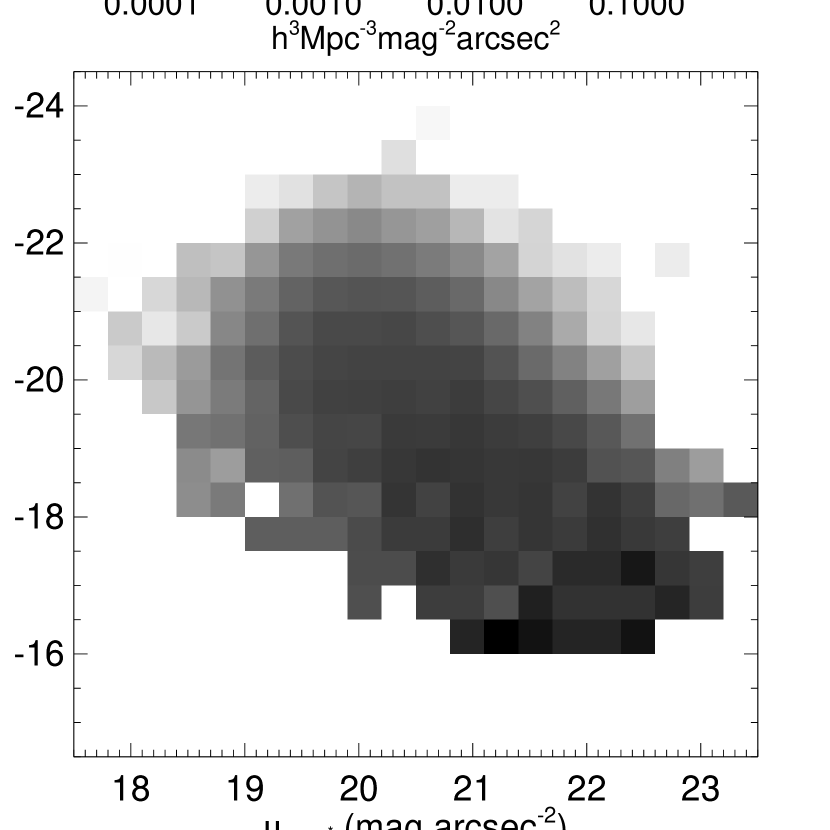
Figure 10: The logarithmic greyscale represents $\hat{\Phi}(M_{r^{\ast}},\mu_{1/2,r^{\ast}})$ in $r^{\ast}$ for SDSS galaxies, in units of galaxies per $h^{-3}$ Mpc³ per unit magnitude per unit surface brightness, calculated using the method of Efstathiou, Ellis, & Peterson (1988). The translation of the greyscale to these units is given in the bar at the top of the figure. The data sample has an explicit half-light surface brightness cut at $\mu_{1/2,r^{\ast}}=23.5$. The strong correlation between surface brightness and luminosity is apparent. It is clear why many of the objects with $\mu_{1/2,r^{\ast}}>22.5$ are low luminosity, as shown in Figure 9.

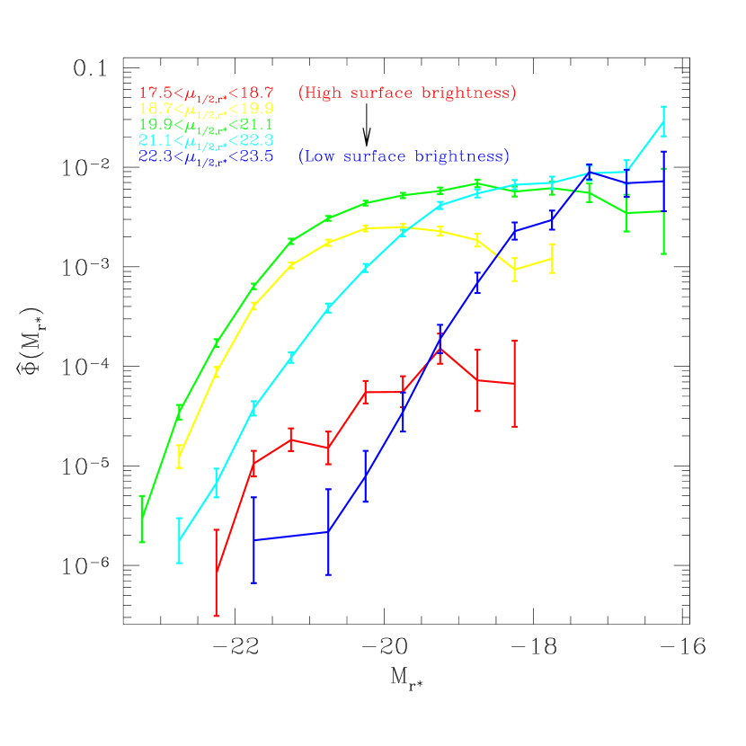
Figure 11: Luminosity function of SDSS galaxies in the $r^{\ast}$ band, in bins of half-light surface brightness, in units of galaxies per $h^{-3}$ Mpc³ per unit magnitude. Each curve shows the luminosity function for a range of surface-brightnesses. As labeled, the curves are colored blue, cyan, green, yellow, and red from high to low surface brightness. The steep faint-end slope for low surface-brightness galaxies is apparent, as well as the fact that the high surface-brightness galaxies tend to be luminous.

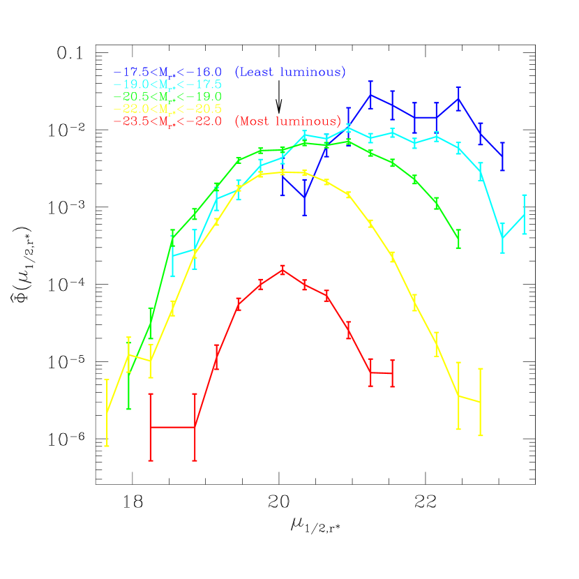
Figure 12: Half-light surface-brightness function of SDSS galaxies in the $r^{\ast}$ band, in bins of galaxy luminosity, in units of galaxies per $h^{-3}$ Mpc³ per unit surface brightness. Each curve shows the surface brightness function for a range of $M_{r^{\ast}}$. As labeled, the curves are colored blue, cyan, green, yellow, and red from low to high luminosity. The luminous galaxies tend to have a characteristic half-light surface brightness, while low luminosity galaxies have a broad distribution that extends to low surface-brightness.

The joint distribution of surface brightness and luminosity is a valuable diagnostic for understanding surface brightness selection effects and an important quantitative characterization of the galaxy population in its own right (see, e.g. Driver & Cross 2000 and references therein). To define this distribution, we take $\mu_{1/2,r^{\ast}}$ (corrected for cosmological surface brightness dimming) as the measure of surface brightness, and use the two-dimensional version of the non-parametric method of Efstathiou, Ellis, & Peterson (1988) to calculate the joint distribution of $\mu_{1/2,r^{\ast}}$ and $M_{r^{\ast}}$, taking into account the apparent magnitude and surface brightness limits of the sample. The results of this fit are shown in Figure 10. Figures 11 and 12 show slices parallel to the axes of this two-dimensional plane: the luminosity function for several ranges of intrinsic surface brightness (Figure 11) and the surface brightness distribution for several ranges of absolute magnitude (Figure 12). Note that we have not corrected the values of $\mu_{1/2,r^{\ast}}$ for the effects of seeing, so the surface brightness of smaller galaxies is systematically underestimated.

Figures 10—12 demonstrate a number of interesting points. Galaxies with $M_{r^{\ast}}<-19$ show a clear peak in their surface brightness distribution, with typical $\mu_{1/2,r^{\ast}}\approx 20$. This result is in rough agreement with the previous results of Freeman (1970) and Courteau (1996), although those authors measured the central, rather than the half-light, surface brightness, and concerned themselves only with disk galaxies. In addition, galaxy surface brightness is clearly correlated with luminosity, in agreement with the results of, e.g., de Jong & Lacey (2000). For lower luminosities, the typical surface brightness is lower, and the distribution of surface brightness is broader (Phillipps & Disney 1986). For lower surface brightness, the galaxy luminosity function becomes steeper. The intrinsic surface brightness distribution of galaxies with $M_{r^{\ast}}<-19$ drops off well before our threshold of $\mu_{1/2,r^{\ast}}=23.5$, providing further evidence that our luminosity function is unaffected by surface brightness selection in this magnitude range. For galaxies less luminous than $M_{r^{\ast}}\approx-17.5$, the surface brightness distribution does decline before hitting our threshold, but not in as definitive a manner as it does for more luminous galaxies; thus, our galaxy density in this regime might be underestimated, and we cannot rule out an upturn in the luminosity function at these magnitudes. However, the luminosity density for a Schechter luminosity function with $\alpha>-2$ is dominated by galaxies with $M\approx M_{\ast}$. Unless there is a radical change in the shape of the luminosity function at $M_{r^{\ast}}>-17.5$, we can safely say that low surface brightness galaxies make a relatively small contribution to the luminosity density of the universe. All of these conclusions are in broad agreement with most recent studies (Impey & Bothun 1997).

There is great potential for further studies of galaxy surface brightness and its correlation with other properties using the SDSS. As a result of improvements in the photometric data reduction software, the main survey (now underway) will adopt a fainter surface brightness threshold, $\mu_{1/2,r^{\ast}}=24.5$. This change will improve the measurement of the luminosity function and the bivariate luminosity-surface brightness distribution at lower luminosities. With the aid of simulated data, it should be possible to correct estimated $\mu_{1/2}$ values for seeing effects. With a larger data sample, it will be possible to analyze joint distributions of surface brightness with a larger set of other galaxy parameters, such as color and morphology, using all five bandpasses. Finally, the SDSS imaging will provide an excellent data set for finding candidate galaxies far below the $\mu_{1/2,r^{\ast}}=24.5$ threshold, even if their redshifts are not obtained by the SDSS spectroscopic survey. Follow-up efforts in optical and 21 cm and correlation with HI radio surveys such as HIPASS (e.g., Banks et al. 1999) will greatly improve the characterization of the low surface brightness galaxy population.

4.4 Dependence of Luminosity on Color

It is well-known that galaxies of different intrinsic colors have quite different luminosity functions. We explore this issue here in a simple way, by calculating the joint distribution of luminosity and the intrinsic $g^{\ast}-r^{\ast}$ color. We determine the intrinsic $g^{\ast}-r^{\ast}$ color for a galaxy at a particular redshift by using the observed $g^{\ast}-r^{\ast}$ color to interpolate between the predicted colors at that redshift for various galaxy types in the results of Fukugita, Shimasaku, & Ichikawa (1995). There are only five templates between which we are interpolating, which may affect the accuracy of our color estimates (typical color corrections to rest frame are about 0.25 magnitudes, so our accuracy is considerably better than that).

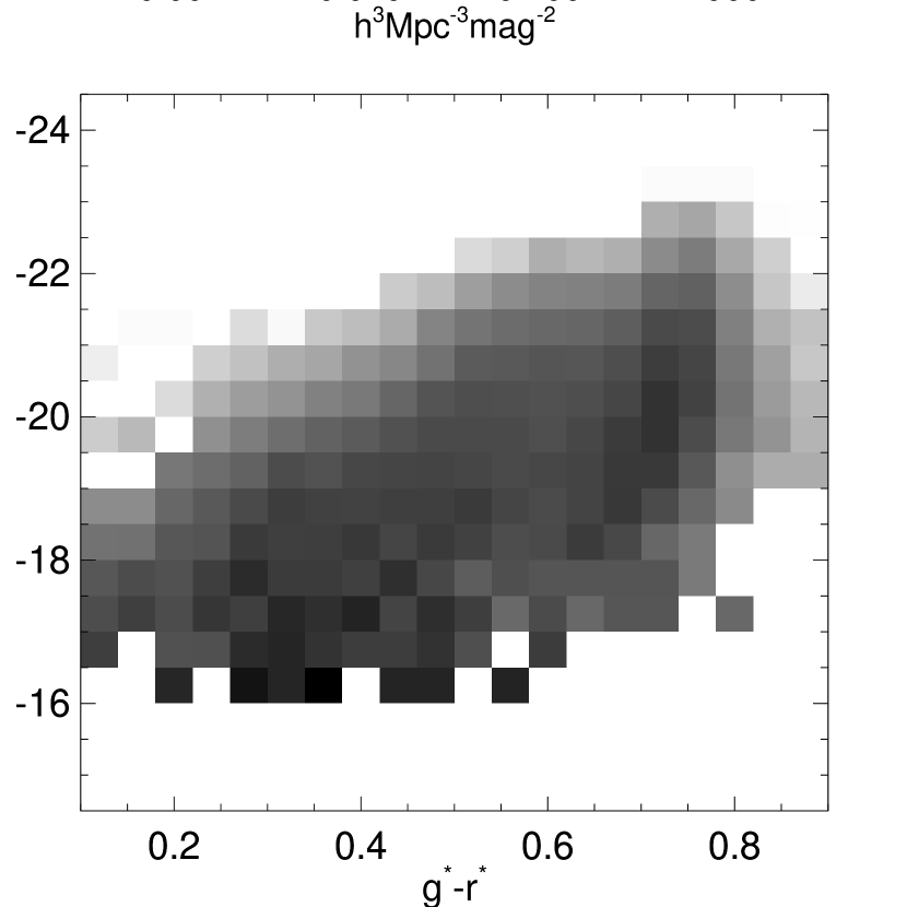
Figure 13: Same as Figure 10, for the joint luminosity-color distribution $\hat{\Phi}(M_{r^{\ast}},g^{\ast}-r^{\ast})$ in $r^{\ast}$ for SDSS galaxies, now in units of galaxies per $h^{-3}$ Mpc³ per unit magnitude per unit color. The intrinsic $g^{\ast}-r^{\ast}$ colors are inferred using the observed $g^{\ast}-r^{\ast}$ color, the measured redshift, and the results of Fukugita, Shimasaku, & Ichikawa (1995). The “E/S0” ridge at $g^{\ast}-r^{\ast}\approx 0.75$ is apparent, as is the strong correlation between luminosity and color.

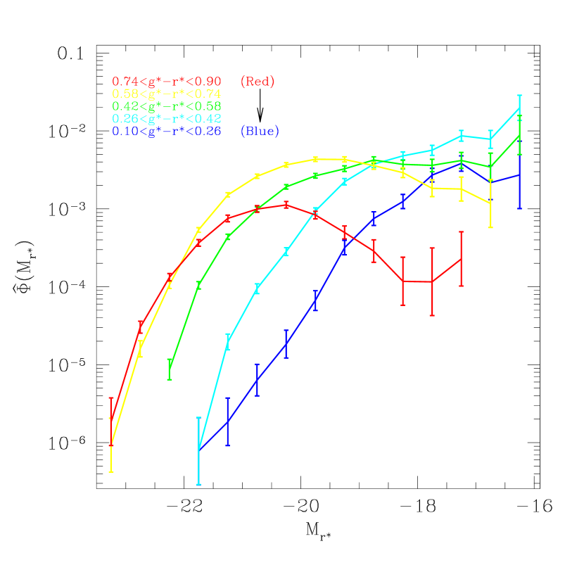
Figure 14: Same as Figure 11, only now showing the luminosity function in bins of intrinsic $g^{\ast}-r^{\ast}$ color, in units of galaxies per $h^{-3}$ Mpc³ per unit magnitude. As labeled, the curves are colored blue, cyan, green, yellow, and red from bluest to redder. The intrinsic color is determined using the observed color, the measured redshift, and the results of Fukugita, Shimasaku, & Ichikawa (1995). Errors in the calibration used for this data probably broaden this distribution slightly, by about 0.05 magnitudes.

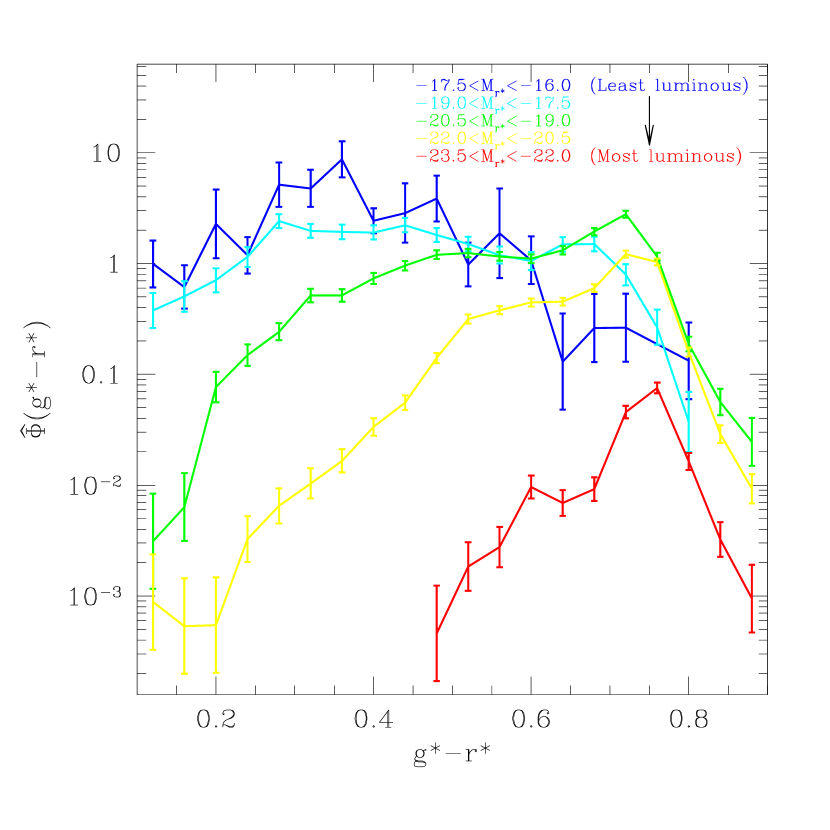
Figure 15: Same as Figure 12, only now showing the distribution of intrinsic $g^{\ast}-r^{\ast}$ color for several ranges of $r^{\ast}$ luminosity, in units of galaxies per $h^{-3}$ Mpc³ per unit color. As labeled, the curves are colored blue, cyan, green, yellow, and red from low to high luminosity. As in Figure 13, the “E/S0” ridge at $g^{\ast}-r^{\ast}\approx 0.75$ is apparent for high luminosities, while for low luminosities, the $g^{\ast}-r^{\ast}$ distribution is nearly flat.

The resulting distribution, $\hat{\Phi}(M_{r^{\ast}},(g^{\ast}-r^{\ast})_{0})$ is shown in Figure 13. This figure shows the “E/S0” ridge at $(g^{\ast}-r^{\ast})_{0}\sim 0.75$, which is well-known in the context of galaxy clusters, as well as the dependence of color on luminosity. As in the case of surface brightness, we show the luminosity function for several ranges of color in Figure 14, and the color distribution as a function of luminosity in Figure 15. The ridge at $(g^{\ast}-r^{\ast})_{0}\sim 0.75$ is apparent at high luminosities in Figure 15, as is the relative flatness of the color distribution at low luminosity.

A better examination of the dependence of galaxy color on luminosity will be possible once the photometric calibration of the data is complete (although the calibrations used here are thought to be accurate to 0.05 magnitudes). Once the final calibration is available, another improvement will be to use the broad-band imaging (and possibly the spectra) to determine the $K$-corrections from the data itself. Methods developed for photometric redshifts, which can use the broad-band colors to reconstruct the typical spectral energy distributions of galaxies (e.g., Csabai et al. 2000), can be brought to bear on this problem and will resolve the difficulties mentioned above associated with the small number of templates used for interpolation.

4.5 Dependence of Luminosity on Morphology

Finally, let us consider the dependence of luminosity on the morphology of galaxies. Although there are numerous ways to quantify galaxy morphology, we choose here for simplicity to use the “concentration index,” defined to be $c=r_{90}/r_{50}$, the ratio of the radii containing 90% and 50% of the Petrosian flux. We will actually study the inverse concentration index $1/c$ here, because it has the property of being between zero and one. The concentration index is high ($c\approx 3.3$, or $1/c\approx 0.3$) for pure de Vaucouleurs profile galaxies and low ($c\approx 2.3$, or $1/c\approx 0.43$) for pure exponential profiles. It has been shown to correlate well with visual morphological classification for bright galaxies (Shimasaku et al., in preparation; Strateva et al., in preparation).

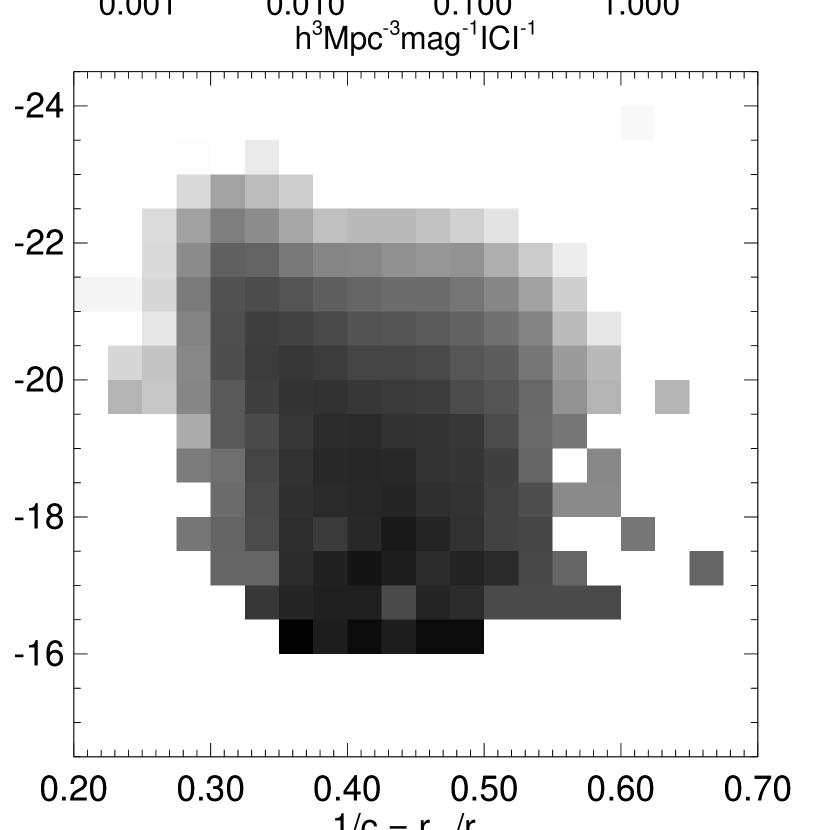
Figure 16: Same as Figure 10, for the joint distribution of luminosity and inverse concentration index $\hat{\Phi}(M_{r^{\ast}},1/c)$ in $r^{\ast}$ for SDSS galaxies, in units of galaxies per $h^{-3}$ Mpc³ per unit magnitude per unit inverse concentration index (ICI). The concentration index is defined to be $c=r_{90}/r_{50}$. Again, the galaxies with a low inverse concentration index (i.e., those galaxies with profiles closer to de Vaucouleurs) tend to be brighter. Note, however, the abundance of high inverse concentration index galaxies ($1/c>0.45$). Since exponential disks should have inverse concentration indices around 0.43, these galaxies either have much broader profiles than exponential, or are being affected by seeing and noise in the measurement. Nevertheless, the trend of luminosity with morphology is clear.

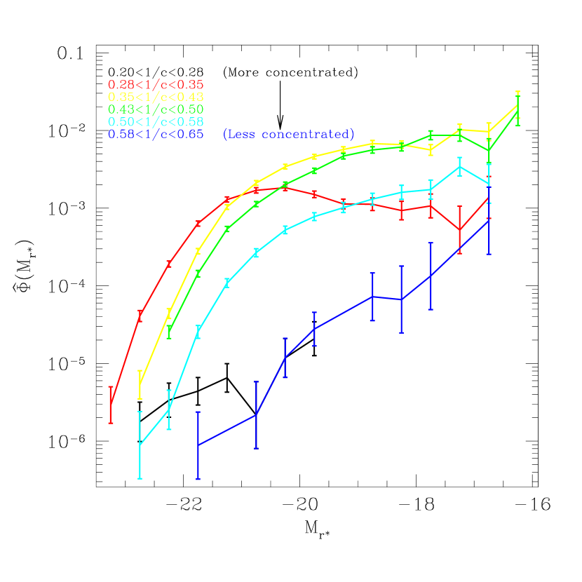
Figure 17: Same as Figure 11, only now showing the luminosity function in bins of inverse concentration index $1/c=r_{50}/r_{90}$, in units of galaxies per $h^{-3}$ Mpc³ per unit magnitude. As labeled, the curves are colored blue, cyan, green, yellow, red, and black from least to most concentrated.

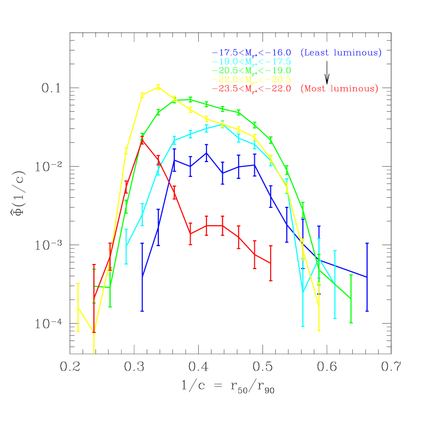
Figure 18: Same as Figure 12, only now showing the distribution of inverse concentration index $1/c=r_{50}/r_{90}$ for several ranges of $r^{\ast}$ luminosity, in units of galaxies per $h^{-3}$ Mpc³ per unit inverse concentration index. As labeled, the curves are colored blue, cyan, green, yellow, and red from low to high luminosity.

Figure 16 shows the joint distribution of luminosity and inverse concentration index. As one might expect, the high luminosity galaxies tend to have high concentration index, and thus to have profiles which are closer to de Vaucouleurs profiles. As before, we slice this two-dimensional plane to get the luminosity function for several ranges of the inverse concentration index in Figure 17, and the distribution of the inverse concentration index for several ranges of luminosity in Figure 18.

Bear in mind that the concentration index is not the only, and perhaps not the best, measure of morphology. For example, some of the inverse concentration indices measured may be artificially affected by the effects of seeing. The inverse concentration index for a realistic PSF measured from the survey is around $1/c\sim 0.5$, so exponential disks and de Vaucouleurs profiles that are marginally resolved will tend to have their inverse concentration indices increased towards this value. Furthermore, this measure of morphology is based only on the radial profile in $r^{\ast}$, and thus does not use the information on color gradients, shape, and galaxy substructure that is available in the imaging. Developing measures of morphology that use the full information from the galaxy images and that are independent of the effects of seeing is one of the ongoing projects within the SDSS collaboration.

5 Comparison of Petrosian Magnitudes to Isophotal Magnitudes

As discussed in Section 2.4, we have selected spectroscopic targets and calculated galaxy luminosities using Petrosian magnitudes, so that the fraction of a galaxy’s light that is measured is independent of the amplitude of its surface brightness profile and independent of cosmological redshift dimming or Galactic extinction. In order to compare our luminosity function results to those of previous surveys, most of which selected galaxies according to some variant of an isophotal magnitude, we must understand how the difference between Petrosian and isophotal magnitudes affects the determination of the luminosity function.

We can calculate an isophotal magnitude for each galaxy in our sample, by integrating the azimuthally-averaged radial profile of each galaxy, which is available as a standard output of photo (Lupton et al., in preparation), out to a chosen isophote. These magnitudes do not correspond exactly to the common definition of isophotal magnitudes, which typically are not azimuthally-averaged. However, as we show in the next section by comparing the SDSS results to those of other surveys, the two definitions are probably nearly equivalent, at least for luminosity statistics.

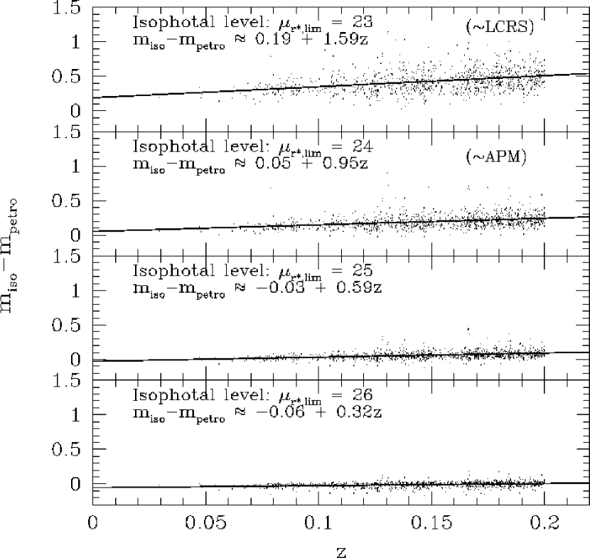
Figure 19: Comparison of isophotal and Petrosian magnitudes as a function of redshift in the $r^{\ast}$ band for several choices of the isophotal limit. We only show galaxies luminous enough to be included in the sample out to $z=0.2$ ($M_{r^{\ast}}<-21.7$). We have quantified the dependence on redshift with a linear regression along $z$.

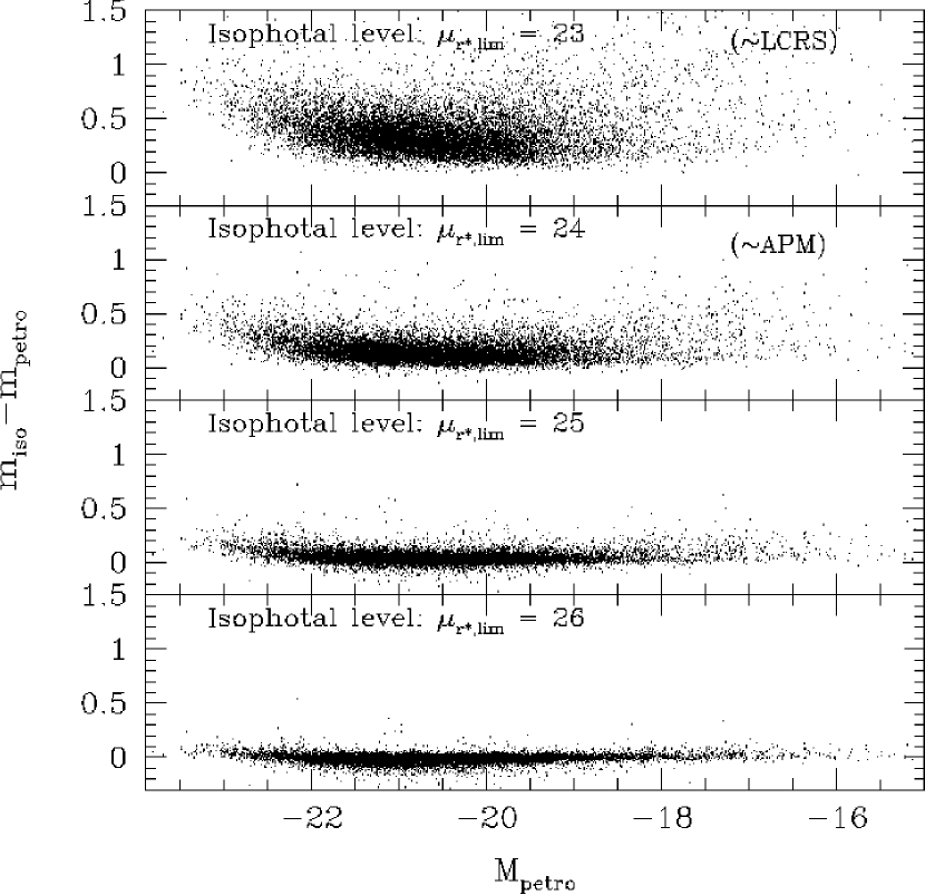
Figure 20: Comparison of isophotal and Petrosian magnitudes as a function of absolute magnitude in the $r^{\ast}$ band for several choices of the isophotal limit. We show all galaxies with $r^{\ast}<17.6$. The most luminous galaxies have high $m_{\mathrm{iso}}-m_{\mathrm{petro}}$ because they tend to be further away, and thus suffer relatively more surface brightness dimming. The least luminous galaxies have high $m_{\mathrm{iso}}-m_{\mathrm{petro}}$ because they tend to be low surface brightness.

Before selecting galaxies according to our newly defined isophotal magnitudes and calculating a luminosity function, let us first directly examine the relationship between the SDSS Petrosian magnitudes and isophotal magnitudes. If $m_{\mathrm{iso}}-m_{\mathrm{petro}}$ were the same for all galaxies, the luminosity scale would differ in the zero-point, but there would be no other change in the shape of the luminosity function. However, $m_{\mathrm{iso}}-m_{\mathrm{petro}}$ depends on both surface brightness (because low surface brightness objects hide a higher fraction of their light below any given isophotal level) and redshift (because of cosmological surface brightness dimming); thus the resulting luminosity function is strongly affected. To show the redshift dependence, Figure 19 shows $m_{\mathrm{iso}}-m_{\mathrm{petro}}$ for a volume-limited sample of galaxies to $z=0.2$ (roughly $M_{r^{\ast}}<-21.7$), for several choices of the isophotal limit. In each panel we show a linear regression fit, showing clearly that the isophotal flux is not a constant fraction of the Petrosian flux as a function of redshift. Figure 20 shows $m_{\mathrm{iso}}-m_{\mathrm{petro}}$ as a function of absolute magnitude. For luminous galaxies, $m_{\mathrm{iso}}-m_{\mathrm{petro}}$ is large because most such galaxies are near the edges of the survey (because more volume is there) and thus suffer considerable surface brightness dimming. For underluminous galaxies, $m_{\mathrm{iso}}-m_{\mathrm{petro}}$ is again large, now because (as dictated by the correlation of luminosity and surface brightness found in Section 4.3) many of these objects are low surface brightness. The redshift and luminosity dependence persists even at isophotal limits so faint that the typical redshift zero isophotal magnitude is brighter than the same galaxy’s Petrosian magnitude. For isophotal limits more typical of other surveys, such as $\mu_{r^{\ast},\mathrm{iso}}=23$, which is comparable to that of the LCRS, or at $\mu_{r^{\ast},\mathrm{iso}}=24$, which under the assumption that ${\langle{b_{j}-r^{\ast}}\rangle}\approx 1$ is comparable to the 2dFGRS, the trend with redshift is quite strong. In Section 6, we will perform a much more careful comparison of our results to those of the LCRS and the 2dFGRS.

Figure 21 compares the luminosity functions derived using the isophotal and the Petrosian samples in the $r^{\ast}$ band. Clearly there is a considerable difference between the estimates, which is not attributable to a simple constant offset between isophotal and Petrosian magnitudes. Instead, the isophotal magnitude estimate differs from the Petrosian magnitude estimate at the low and high luminosity ends. Figure 21 also lists $f_{\mathrm{lum}}$, the fraction of the integrated luminosity density in the Petrosian sample that is recovered in each isophotal sample. From these results, we infer that surveys with shallower isophotal limits could be missing considerable amounts of luminosity density. We will compare our results more directly to other surveys (and in the appropriate bands) in Section 6 below.

There are two reasons that isophotal samples can underestimate the luminosity density when the isophotal limits are too bright. First, isophotal magnitudes with bright limits measure less flux for each galaxy, as revealed by Figure 20. Second, because the fraction of the total flux measured by an isophotal magnitude decreases with redshift from cosmological surface brightness dimming, using the standard formula for the distance modulus overestimates the effective volume of each galaxy (Dalcanton 1998). The dominant effect in Figure 21 is the first, that less light is measured. To show this, we recalculate luminosity functions using a simple $1/V_{\mathrm{max}}$ estimator (e.g., Binggeli, Sandage & Tammann 1988). We first use the Petrosian magnitudes both to determine the absolute magnitude of the galaxy and to apply the flux limits (and thus also to determine $V_{\mathrm{max}}$). Then we use the isophotal magnitudes to do both, finding the expected reduction in luminosity density (about 40% in the case of $\mu_{r^{\prime},\mathrm{lim}}=23$). We then calculate the luminosity function again, determining $M_{r^{\ast}}$ from the isophotal magnitude but applying the flux limits to the Petrosian magnitude. In this case, the reduction of the luminosity density is nearly as great, around 35%. Finally, we determine $M_{r^{\ast}}$ from the Petrosian magnitude, but apply the flux limits to the isophotal magnitude, thus isolating the effect of an incorrect $V_{\mathrm{max}}$ determination. In the case that $\mu_{r^{\prime},\mathrm{lim}}=23$, this procedure reduced the luminosity density only by 10%. These results show that it is the missing light beyond the isophotes that dominates the reduction in the luminosity density, rather than an overestimate of the maximum volume. Presumably, this result is related to that of Dalcanton (1998), that the systematic effects associated with isophotal magnitudes have only a moderate effect on the estimated $V/V_{\mathrm{max}}$ distribution. The error in $V_{\mathrm{max}}$ estimated with the standard distance modulus may be large in some individual cases, but most galaxies enter the sample at a redshift close to the largest one at which it is possible for them to, because that is where most of the volume is. The additional dimming out to the galaxy’s limiting redshift is therefore small in most cases.

6 Comparison to Other Surveys

As we have seen above, the choice of isophotal magnitudes can greatly affect the results for the galaxy luminosity function, confirming the results of Dalcanton (1998). Thus, in order to show that the results of the SDSS are consistent with those of other surveys, we must reanalyze the SDSS data in the same ways that previous surveys analyzed their data. The SDSS provides the ability to do so (for surveys of comparable depth) in a way that no other large-scale survey has before. Using the five-band color information and the color conversions for galaxies provided by Fukugita, Shimasaku, & Ichikawa (1995), one can convert the SDSS magnitudes into the appropriate band for almost any desired optical survey. We convert to the LCRS $R$ band and to $b_{j}$, and compare to the LCRS and 2dFGRS luminosity functions, finding significantly more luminosity density in both cases. Using the measured photometric properties, one can reconstruct an isophotal magnitude similar to that of any given survey (albeit with azimuthally averaged light profiles). When we do so for the LCRS and for 2dFGRS, we find our results are consistent with theirs. These results demonstrate that the LCRS and 2dFGRS are missing significant fractions of the light in the universe because their measurements of galaxy magnitudes are based on fairly bright isophotes.

6.1 Comparison to the LCRS

The LCRS photometry is expressed in its own variant of the $R$ band, a hybrid of Gunn $r$ and the Kron-Cousins $R$ band, which we will denote $R_{\mathrm{GKC}}$ following Shectman et al. (1996). This band can be related to SDSS magnitudes as follows (Fukugita, Shimasaku, & Ichikawa 1995; Shectman et al. 1996):

$$R_{\mathrm{GKC}}=r^{\ast}-0.05-0.089(g^{\ast}-r^{\ast}).$$ (18)

We use this transformation to calculate $R_{\mathrm{GKC}}$-band Petrosian magnitudes for all SDSS galaxies, corrected for Galactic extinction. Using the method described in Section 3 for defining complete samples in $u^{\ast}$, $g^{\ast}$, $i^{\ast}$ and $z^{\ast}$, we define a complete sample in $R_{\mathrm{GKC}}$ by setting a flux limit of $m_{\mathrm{lim}}=17.40$. For consistency with Lin et al. (1996), who calculate the $R_{\mathrm{GKC}}$-band luminosity function in the LCRS, we use an Einstein-de Sitter universe in this case. The results are listed in Table 3. The top panel of Figure 22 shows the $R$-band luminosity function determined from the SDSS in this way and compares our result to that of Lin et al. (1996). The two luminosity functions diverge at low and high luminosities for the reasons discussed in Section 5: isophotal magnitudes underestimate the luminosities of low luminosity galaxies because of their low intrinsic surface brightnesses, and of high luminosity galaxies because of cosmological surface brightness dimming. The ratio of the $R$-band luminosity density found by Lin et al. (1996) to that found here is $f_{\mathrm{lum}}=0.48$. That is, there is (at least) twice as much $R_{\mathrm{GKC}}$-band light in the universe than found by the LCRS. Table 3 lists these results, along with the conversions of the luminosity densities to solar units (assuming $M_{R_{\mathrm{GKC}}\odot}=4.52$, using the results of Binney & Merrifield 1998 and the relation $R_{\mathrm{GKC}}=R_{\mathrm{KC}}+0.1$ from Shectman et al. 1996; these choices are consistent with the results quoted by Lin et al. 1996).

Let us now analyze the SDSS images using the same method as used in the LCRS. First, we use isophotal magnitudes limited at $\mu_{R_{\mathrm{GKC}},\mathrm{lim}}=23$; this number approximately corresponds to the statement of Shectman et al. (1996) that the LCRS isophotal magnitudes are limited at 15% of the sky brightness. Second, Shectman et al. (1996) exclude galaxies of low “central surface brightness,” as measured by the magnitude within a fixed angular aperture about the size of a fiber. Similarly, we apply a “central surface brightness” cut based on the “fiber magnitude,” an aperture magnitude with a $3^{\prime\prime}$ diameter. Following Shectman et al. (1996), we define the fiber magnitude cut to be:

$$m_{R_{\mathrm{GKC}},\mathrm{fiber}}<18.85-0.5(17.7-m_{R_{\mathrm{GKC}}}),$$ (19)

Finally, for consistency we calculate the $K$-corrections using the formula $K(z)=2.5\log_{10}(1+z)$, as Lin et al. (1996) did (although this makes rather little difference in our results). The bottom panel of Figure 22 shows the comparison of the resulting luminosity function to that of Lin et al. (1996). They are largely consistent, except that the SDSS sample has a slightly brighter $M_{\ast}$; this difference may persist because our isophotal limit is not precisely what LCRS used. Nevertheless, the general consistency shows that the extra flux detected in the SDSS in the top panel is most likely real, and that the missing light in the LCRS is due to having shallow isophotes and excluding galaxies with low central surface brightnesses. To understand how much is due to the central surface brightness cut of Equation (19), we list results in Table 3 for the case in which we do not apply this cut; this test indicates that the central magnitude cut is responsible for a substantial portion of the underestimate in the luminosity density.

6.2 Comparison to the 2dFGRS

The 2dFGRS sample is based on APM plates (Maddox, Efstathiou, & Sutherland 1990) and uses the $b_{j}$ band. Here we relate the SDSS photometry to $b_{j}$ using the relation

$$b_{j}=g^{\ast}+0.14+0.088(g^{\ast}-r^{\ast}),$$ (20)

determined using the results of Fukugita, Shimasaku, & Ichikawa (1995) and the galaxy color relation $b_{j}=B-0.35(B-V)$ from Metcalfe, Fong, & Shanks (1995). We follow the same procedure as for the LCRS in the previous section to create a sample limited at $m_{b_{j},{\mathrm{lim}}}=17.8$. Again, for consistency with Folkes et al. (1999), we assume an Einstein-de Sitter universe. While our results are much closer to those of 2dFGRS than they were to the LCRS, we still measure about 1.4 times the luminosity density that Folkes et al. (1999) do, as we show in Figure 23. This difference is significant, given that the stated errors in the $b_{j}$ luminosity density in the 2dFGRS are about 5%, and the errors for the SDSS are about 15%. Table 3 lists these results, now using $M_{b_{j}\odot}=5.30$ to convert to solar units (determined using the stellar color relation $b_{j}=B-0.28(B-V)$ from Blair & Gilmore 1982 and the results of Binney & Merrifield 1998).

Let us analyze the SDSS images using the methods used by 2dFGRS. APM magnitudes are isophotally limited at $\mu_{b_{j}}=25$ mag per square arcsecond, and then corrected to total magnitudes by assuming that the galaxy profile is a circularly symmetric Gaussian (Maddox et al. 1990). After determining these “APM-like” magnitudes for SDSS galaxies, and applying a flux limit of $m_{b_{j},{\mathrm{lim}}}=17.8$, we again calculate the luminosity function. This flux limit is considerably shallower than that of the 2dFGRS. Thus, the mean redshift is lower, and to accurately match the isophotal limits would require a slightly brighter isophotal limit; we have instead decided to err on the side of including a little more flux. The result is shown in the bottom panel of Figure 23. The SDSS luminosity function determined in this manner is nearly identical to the 2dFGRS luminosity function. (Although the Schechter parameters are rather different, it is clear from the figure that the values are nearly degenerate). Given our estimated errors and the fact that our $b_{j}$ sample is considerably shallower than that of the 2dFGRS, this agreement of the two results is somewhat surprising. This result indicates that the 40% difference in luminosity density between the SDSS and 2dFGRS is due to the fact that the APM isophotal limits exclude a significant amount of light in the outer regions of galaxies, even when corrected. For comparison, we also give results in Table 3 for the case of $b_{j}=25$ isophotal magnitudes, with no correction to “total” magnitudes based on the Gaussian model. These results show that while the APM corrections work in the right direction, the Gaussian model is an insufficient description of observed galaxy profiles for extrapolation to “total” magnitudes.

7 Conclusions

We have presented the luminosity function and luminosity density of galaxies in five optical bandpasses ($u^{\ast}$, $g^{\ast}$, $r^{\ast}$, $i^{\ast}$ and $z^{\ast}$) using $11,275$ galaxies in SDSS commissioning data. The Schechter function appears to be a good fit in all cases, with a low-luminosity slope that is remarkably similar in all bandpasses. On the other hand, the slope $\alpha$ is sensitive to galaxy surface brightness, color, and morphology. The redshift distribution of the galaxies is generally consistent with our derived luminosity function, although large-scale structure is still evident in our sample.

We have demonstrated the correlation between $r^{\ast}$ luminosity and galaxy surface brightness, color, and morphology. In particular, we have shown that luminous galaxies tend to be higher surface brightness, redder, and more concentrated than less luminous galaxies, in accordance with previous results. We find that galaxies obey a strong magnitude-surface brightness relation. There is a high characteristic half-light surface brightness for luminous galaxies; at the same time, low-luminosity galaxies show a broad surface brightness distribution, with many low surface brightness objects. As described above, refinements of the photometric analysis beyond the standard software used for the survey will improve our understanding of these correlations. For example, a better understanding of the effects of seeing, inclination, and internal dust extinction will improve our measures of surface brightness and morphology. Improvements in our estimates of $K$-corrections, which will be possible using both the spectroscopy and the five-band photometry of the SDSS, will improve our understanding of the distribution of galaxy colors and allow us to estimate the stellar mass function of galaxies. Work in progress on the spectral classification of SDSS galaxies (e.g., Castander et al. 2001) is showing the same trends of galaxy type with luminosity found here.

We have shown that a considerable fraction of the luminosity density in the universe has been missed by previous samples that were based on shallower imaging. We measure 2 times the $R_{\mathrm{GKC}}$-band luminosity density found in the LCRS and 1.4 times the $b_{j}$-band luminosity density found in the 2dFGRS. Work in progress, which directly compares the measured magnitudes of galaxies in these surveys to SDSS magnitudes in the regions where the surveys overlap, will test whether these differences are indeed reasonable. While large-scale structure could still have some effect on results from these surveys, our internal tests show that the differences of results are almost certainly due to our adoption of Petrosian magnitudes in preference to isophotal magnitudes. In particular, we can reproduce the LCRS and 2dFGRS results if we mimic their photometry and selection effects. The high luminosity density found by the SDSS implies that the cosmic density of stellar matter $\Omega_{\ast}$ is higher than previously thought. If this is the case, it may relieve some of the strain on galaxy formation models, which typically predict a higher density of stellar matter than previous observational estimates (Katz, Weinberg, & Hernquist 1996; Pearce et al. 1999; Granato et al. 2000).

Our estimates of the luminosity density, given in Tables 2 and 3, are almost certainly still underestimates. First, for the case of de Vaucouleurs profiles, we know that up to 18% of the galaxy light may be missed by the Petrosian magnitudes as we define them. Including this light would increase somewhat the total luminosity density found here (though only by a few percent, because de Vaucouleurs profile galaxies constitute only about 20% of all galaxies). Second, we have shown that while the explicit surface brightness limit $\mu_{1/2,\mathrm{lim}}=23.5$ of the commissioning data exclude only 0.5% of galaxies, these galaxies very likely represent a larger fraction of the luminosity density than that; for example, only 1.5% of galaxies are in the range $22.5<\mu_{1/2,r^{\ast}}<23.5$, but such galaxies are responsible for $\sim$ 5% of the luminosity in the universe. The deeper surface-brightness limit of the main SDSS survey will thus provide a more complete estimate of the luminosity density in the universe. Third, our estimates assume a constant low luminosity slope $\alpha$. An upturn in the luminosity function at absolute magnitudes less luminous than $M=-16$, suggested by some studies (Loveday 1997; Phillipps et al. 1998), would mean there was yet more luminosity not included in this analysis. A final possibility, related to the previous one, is that a significant fraction of stars exist outside of galactic environments, having perhaps been tidally stripped from their galaxy of birth. As more SDSS data is obtained and we perform more sophisticated analyses of the various selection effects in the survey, we will be able to address many of these problems.

Tables of the non-parametric fits to the luminosity function in each band and the joint relationships between luminosity and surface brightness, color, and concentration, are available on the World Wide Web. We expect that these results and the parametric fits in Table 2, which represent a straightforward analysis of only a small fraction (one percent) of the expected SDSS sample, will already provide interesting new constraints on theories of galaxy formation. In addition, this characterization of the luminosities, surface brightnesses, colors, and morphologies of local galaxies provides a solid baseline for interpreting the evolution of galaxies observed at higher redshift. Future work with the SDSS will allow us to explore the correlations between all of these properties and to describe fully the population of galaxies in the local universe.

Table 1: Limits Applied to Sample in Each SDSS Band

Band	Flux Limits	Redshift Limits (km s-1)	Number of Galaxies
$u^{\ast}$	$14.50<m<18.40$	$5,000<cz<30,000$	1,679
$g^{\ast}$	$14.50<m<17.65$	$5,000<cz<50,000$	4,684
$r^{\ast}$	$14.50<m<17.60$	$5,000<cz<60,000$	11,275
$i^{\ast}$	$14.50<m<16.90$	$5,000<cz<60,000$	7,441
$z^{\ast}$	$14.50<m<16.50$	$5,000<cz<60,000$	6,090

Table 2: Parameters of Fits to Luminosity Function in SDSS

$\Omega_{m}$	$\Omega_{\Lambda}$	Band	$\phi_{\ast}$	$M_{\ast}-5\log_{10}h$	$\alpha$	$r_{M_{\ast},\alpha}$	$j$ (mags)	$j$ ($h$ $10^{8}L_{\odot}$)	$f_{\mathrm{np}}$
			($10^{-2}$ $h^{3}$ Mpc-3)
0.3	0.7	$u^{\ast}$	$4.00\pm 0.90$	$-18.34\pm 0.08$	$-1.35\pm 0.09$	0.80	$-15.21\pm 0.26$	$4.35\pm 1.08$	0.85
		$g^{\ast}$	$2.06\pm 0.23$	$-20.04\pm 0.04$	$-1.26\pm 0.05$	0.79	$-16.05\pm 0.13$	$2.81\pm 0.38$	0.94
		$r^{\ast}$	$1.46\pm 0.12$	$-20.83\pm 0.03$	$-1.20\pm 0.03$	0.78	$-16.41\pm 0.09$	$2.58\pm 0.28$	1.00
		$i^{\ast}$	$1.28\pm 0.11$	$-21.26\pm 0.04$	$-1.25\pm 0.04$	0.77	$-16.74\pm 0.10$	$3.19\pm 0.37$	0.98
		$z^{\ast}$	$1.27\pm 0.11$	$-21.55\pm 0.04$	$-1.24\pm 0.05$	0.74	$-17.02\pm 0.11$	$3.99\pm 0.48$	0.97
0.3	0.0	$u^{\ast}$	$4.48\pm 1.06$	$-18.27\pm 0.07$	$-1.32\pm 0.09$	0.78	$-15.20\pm 0.26$	$4.34\pm 1.07$	0.84
		$g^{\ast}$	$2.48\pm 0.33$	$-19.97\pm 0.05$	$-1.23\pm 0.05$	0.83	$-16.16\pm 0.15$	$3.09\pm 0.47$	0.98
		$r^{\ast}$	$1.71\pm 0.15$	$-20.74\pm 0.03$	$-1.20\pm 0.03$	0.74	$-16.49\pm 0.09$	$2.78\pm 0.31$	0.96
		$i^{\ast}$	$1.47\pm 0.13$	$-21.17\pm 0.04$	$-1.23\pm 0.04$	0.77	$-16.78\pm 0.10$	$3.31\pm 0.39$	0.96
		$z^{\ast}$	$1.45\pm 0.14$	$-21.46\pm 0.04$	$-1.20\pm 0.05$	0.80	$-17.02\pm 0.11$	$3.99\pm 0.48$	1.00
1.0	0.0	$u^{\ast}$	$4.68\pm 1.13$	$-18.24\pm 0.07$	$-1.31\pm 0.09$	0.82	$-15.20\pm 0.26$	$4.34\pm 1.10$	0.84
		$g^{\ast}$	$2.42\pm 0.30$	$-19.92\pm 0.04$	$-1.22\pm 0.05$	0.80	$-16.07\pm 0.13$	$2.87\pm 0.40$	0.97
		$r^{\ast}$	$1.87\pm 0.18$	$-20.67\pm 0.03$	$-1.15\pm 0.03$	0.84	$-16.47\pm 0.10$	$2.74\pm 0.31$	1.00
		$i^{\ast}$	$1.61\pm 0.15$	$-21.11\pm 0.04$	$-1.20\pm 0.05$	0.78	$-16.78\pm 0.11$	$3.32\pm 0.40$	0.98
		$z^{\ast}$	$1.62\pm 0.16$	$-21.39\pm 0.04$	$-1.19\pm 0.05$	0.74	$-17.08\pm 0.11$	$4.19\pm 0.51$	0.96

Note. — Luminosity function in various bands assuming the three cosmological models considered here, with $H_{0}=100$ km s^-1. The Schechter function is characterized by the three parameters $\phi_{\ast}$ (in units of $10^{-2}$ $h^{3}$ Mpc^-3), $M_{\ast}$, and $\alpha$, whose values and errors in each case are listed here. Also listed is the covariance between the errors of $M_{\ast}$ and $\alpha$, determined from the Monte Carlo error determination. $j$ is the luminosity density as determined by integrating the Schechter function over all luminosities (again in units of $h^{3}$ Mpc^-3). We list $j$ both in absolute magnitudes and in solar luminosities (determined as described in the text). The error bars on the value of $j$ in solar luminosities include a 7% contribution due to calibration and color transformation uncertainties. $f_{\mathrm{np}}$ is the fraction of the luminosity in the extrapolated Schechter function which is accounted for in the non-parametric fit; that is, this is the fraction of the inferred light which comes from galaxies with luminosities which are observed in the sample. Naturally, it is lowest when the slope $\alpha$ at low luminosities is highest.

Table 3: Comparison of SDSS Luminosity Function to 2dFGRS and LCRS

Band	Sample	$\phi_{\ast}$	$M_{\ast}-5\log_{10}h$	$\alpha$	$j$ (mags)	$j$ ($h$ $10^{8}L_{\odot}$)
		($10^{-2}$ $h^{3}$ Mpc-3)
$R_{\mathrm{G;K-C}}$	SDSS Petrosian	$1.92\pm 0.23$	$-20.80\pm 0.03$	$-1.17\pm 0.03$	$-16.64\pm 0.12$	$2.91\pm 0.38$
	SDSS Isophotal	$2.13\pm 0.26$	$-20.37\pm 0.04$	$-0.94\pm 0.05$	$-16.15\pm 0.12$	$1.86\pm 0.24$
	SDSS Isophotal	$2.02\pm 0.24$	$-20.30\pm 0.04$	$-0.74\pm 0.05$	$-15.95\pm 0.12$	$1.54\pm 0.20$
	LCRS	$1.90\pm 0.1$	$-20.29\pm 0.02$	$-0.70\pm 0.03$	$-15.87\pm 0.1$	$1.4\pm 0.1$
$b_{j}$	SDSS Petrosian	$2.69\pm 0.34$	$-19.70\pm 0.04$	$-1.22\pm 0.05$	$-15.97\pm 0.14$	$3.21\pm 0.46$
	SDSS Isophotal	$2.17\pm 0.28$	$-19.55\pm 0.05$	$-1.12\pm 0.06$	$-15.47\pm 0.14$	$2.04\pm 0.30$
	SDSS Isophotal	$2.32\pm 0.30$	$-19.62\pm 0.04$	$-1.15\pm 0.05$	$-15.65\pm 0.13$	$2.39\pm 0.34$
	2dFGRS	$1.69\pm 0.17$	$-19.73\pm 0.06$	$-1.28\pm 0.05$	$-15.56\pm 0.05$	$2.19\pm 0.12$

Note. — Same as Table 2, for the LCRS $R_{\mathrm{G;K-C}}$-band and the $b_{j}$ band. We include comparisons to the LCRS (Lin et al. 1996) and the 2dFGRS (Folkes et al. 1999).

Figure 1: Behavior of Petrosian magnitudes as a function of galaxy size, for pure, face-on exponential profiles (top panel) and circularly symmetric de Vaucouleurs profiles (bottom panel), under marginal seeing conditions in the SDSS. For each profile, the fraction of total light measured by the Petrosian flux is plotted against the (true) angular half-light radius of the galaxy. In the absence of seeing, Petrosian flux measures a constant fraction of the total light as a function of redshift, unlike isophotal fluxes. However, small differences do appear as a function of the angular size due to seeing. As the galaxy size becomes comparable to the size of the seeing disk, the fraction of light measured by Petrosian quantities approaches that fraction for a PSF, which is about 95%. In the case of exponential disks, this reduces the flux, because in the absence of seeing nearly 100% of the light is measured. In the case of a de Vaucouleurs profile, this increases the flux, because in the absence of seeing about 80% of the light is measured (assuming that the de Vaucouleurs profile extends to infinity). As shown in Figure 2, a significant number of galaxies have sizes close to that of the seeing disk, so this dependence on galaxy size for small galaxies (which is present in isophotal magnitudes as well) will limit the accuracy of our estimates of the total luminosity density, though only to a few percent.

Figure 2: Distribution of half-light radii $r_{50}$ of SDSS galaxies with $r^{\ast}<17.6$. Top panel shows the distribution; bottom panel shows the fractional cumulative distribution. Roughly half of the galaxies are in the regime ($r_{50}<2.5^{\prime\prime}$) in which seeing significantly affects the determination of the Petrosian radius and flux.

Figure 3: Distribution of the quantity $m_{\mathrm{PSF}}-m_{\mathrm{model}}$ (determined in $r^{\ast}$), which is used to separate stars from galaxies for the purposes of target selection in the SDSS. The cut-off of 0.242 used in the commissioning data for this purpose is shown as the vertical line. The solid histogram is the distribution of $m_{\mathrm{PSF}}-m_{\mathrm{model}}$ for targeted objects which were spectroscopically identified as galaxies; the dotted histogram is the distribution for targeted objects which were spectroscopically identified as stars. About 1% of objects targeted as galaxies turned out to be stars. The distribution falls off sharply at small $m_{\mathrm{PSF}}-m_{\mathrm{model}}$, implying that $\ll 1\%$ of galaxies brighter than $r^{\ast}=17.6$ are misclassified as stars.

Figure 4: $K$-corrections in the $r^{\ast}$ band for galaxies with intrinsic $g^{\ast}-r^{\ast}$ colors of 0.2, 0.4, 0.6, and 0.8, as labeled. These curves are obtained by linear interpolation between the morphological types used by Fukugita, Shimasaku, & Ichikawa (1995). Similar results are available for the other four bands.

Figure 5: Top panel shows the luminosity function of SDSS galaxies in the $r^{\ast}$ band, based on a sample of $11,275$ galaxies in the commissioning data. For these results, we assumed $\Omega_{m}=0.3$ and $\Omega_{\Lambda}=0.7$. Results for other cosmologies are given in Table 2. The Schechter fit (thick line) and the non-parametric fit (thin line with error bars) agree well. The correlation coefficient between $\alpha$ and $M_{\ast}$ is $r=0.78$, showing that the errors in these parameters are strongly correlated. Bottom panel shows the number of galaxies in each bin used to determine the luminosity function; even though the least luminous galaxies have the highest space density, there are very few such galaxies in a flux-limited sample. The fact that the low-luminosity end of the correlation function is based on a relatively small fraction of the galaxies in the sample is the reason that the errors in the normalization of the luminosity function are not comparable to the Poisson errors expected given the number of galaxies; that is, a small number of the galaxies are given disproportionate statistical weight, making the errors greater than Poisson.

Figure 6: Same as Figure 5, for the $u^{\ast}$, $g^{\ast}$, $i^{\ast}$, and $z^{\ast}$ bands. The flux limits and number of galaxies in each sample are listed in Table 2. As in the $r^{\ast}$ luminosity function in Figure 5, the Schechter fits (thick line) and the non-parametric fits (thin line with error bars) agree well.

Figure 7: Redshift distribution of SDSS galaxies (histogram) compared to the average distribution expected given the $r^{\ast}$ luminosity function and the flux limits (using $K$-corrections for a “typical” galaxy color of $g^{\ast}-r^{\ast}=0.65$). The redshift distribution is reasonable, although large-scale structure is obvious.

Figure 8: Comparison of the luminosity function in $r^{\ast}$ determined using samples above and below $cz=30,000$ km s^-1. In the region in which the two luminosity functions overlap they are in good agreement, indicating that the redshift dependence of the selection function is purely due to the flux limits of the survey. More precise tests of this nature can be made when larger areas of the sky (which are less affected by large-scale structure) become available.

Figure 9: Luminosity function of SDSS galaxies in the $r^{\ast}$ band for the full sample, limited at a surface-brightness of $\mu_{1/2,r^{\ast}}<23.5$, and for a restricted sample with $\mu_{1/2,r^{\ast}}<22.5$. The higher surface brightness threshold excludes about 1.5% of the galaxies in the full sample. The top panel shows both luminosity functions, showing that differences between them appear at $M_{r^{\ast}}>-19$. The bottom panel shows the ratio of the two luminosity functions.

Figure 21: Fitted $r^{\ast}$ luminosity function for Petrosian magnitudes (upper curve in each panel, same as Figure 5) compared to the luminosity function using isophotal magnitudes (lower curve in each panel). Each panel corresponds to a different choice of limiting isophotal surface-brightness $\mu_{r^{\ast},\mathrm{lim}}$, as labeled. The Schechter function parameters for each choice of isophotal limit are listed in each panel, as well as the fraction $f_{\mathrm{lum}}$ of the total Petrosian luminosity that is detected in each isophotal sample.

Figure 22: $R$-band luminosity function in the SDSS compared to that in the LCRS calculated by Lin et al. (1996). Top panel shows the luminosity function calculated from the SDSS using Petrosian magnitudes. The ratio of the $R$-band luminosity density in the LCRS to that in the SDSS is $f_{\mathrm{lum}}=0.48$. The bottom panel shows the results of analyzing the SDSS data in the same manner as the LCRS, using isophotal magnitudes limited at $\mu_{R,\mathrm{lim}}=23$ and applying a central magnitude cut similar to that of the LCRS, as described in the text. This sample is considerably more similar to the results of the LCRS itself. The remaining discrepancies may be due to our use of a slightly deeper isophotal magnitude than that of the LCRS, the axisymmetric nature of our isophotal magnitudes, or the slightly different definition of our central magnitude cut.

Figure 23: Same as Figure 22, this time comparing the SDSS $b_{j}$ luminosity function to that of the 2dFGRS as calculated by Folkes et al. (1999). The top panel shows that the SDSS sample based on Petrosian magnitudes has about 1.4 times the luminosity density of the 2dFGRS luminosity function. The bottom panel shows that if we use isophotal magnitudes with the same isophotal limit that the 2dFGRS uses, and “correct” these magnitudes in the same manner as they do, we obtain nearly the same results. These results indicate that the 2dFGRS misses a significant amount of luminosity density due to its relatively shallow isophotal limits, notwithstanding the efforts to correct the isophotal magnitudes assuming a universal Gaussian profile for galaxies.

References

- Banks et al. (1999) Banks, G. D., Disney, M. J., Knezek, P. M., Jerjen, H., Barnes, D. G., Bhatal, R., de Blok, W. J. G., Boyce, P. J., Ekers, R. D., Freeman, K. C., Gibson, B. K., Henning, P. A., Kilborn, V., Koribalski, B., Kraan-Korteweg, R. C., Malin, D. F., Minchin, R. F., Mould, J. R., Oosterloo, T., Price, R. M., Putman, M. E., Ryder, S. D., Sadler, E. M., Staveley-Smith, L., Stewart, I., Stootman, F., Vaile, R. A., Webster, R. L., Wright, A. E. 1999, ApJ, 524, 612
- Binggeli, Sandage & Tammann (1988) Binggeli, B., Sandage, A., & Tammann, G. A. 1988, ARA&A, 26, 509
- Binney & Merrifield (1998) Binney, J., & Merrifield, M. 1998, Galactic Astronomy (Princeton: Princeton University Press)
- Blair & Gilmore (1982) Blair, M., & Gilmore, G. 1982, PASP, 94, 742
- Castander et al. (2001) Castander, F., et al. SDSS Collaboration 2001, AJ, submitted
- Colless (1999) Colless M. M., 1999, in Wide Field Surveys in Cosmology, eds. S. Colombi, Y. Mellier, & B. Raban, 14th IAP Colloquium, Editions Frontieres, pp.77-80
- Courteau (1996) Courteau, S. 1996, ApJS, 103, 363
- Csabai et al. (2000) Csabai, I., Connolly, A. J., Szalay, A. S., & Budavári, T. 2000, AJ, 119, 69
- Dalcanton (1998) Dalcanton, J. J. 1998, ApJ, 495, 251
- Davis & Huchra (1982) Davis, M., & Huchra, J. 1982, ApJ, 254, 437
- de Jong & Lacey (2000) de Jong, R. S., & Lacey, C. 2000, ApJ, 545, 781
- Driver (1999) Driver, S. P. 1999, ApJ, 526, L69
- Driver & Cross (2000) Driver, S. P., & Cross, N. 2000, in Mapping the Hidden Universe, eds. R. C. Kraan-Korteweg, P. A. Henning, H. Andernach, ASP Conference Series (astro-ph/0004201)
- Efstathiou, Ellis, & Peterson (1988) Efstathiou, G., Ellis, R. S., & Peterson, B. S. 1988, MNRAS, 232, 431
- Fan (1999) Fan, X. 1999, AJ, 117, 2528
- Fan et al. (2001) Fan, X., et al. SDSS Collaboration 2001, submitted to AJ (astro-ph/0008122)
- Folkes et al. (1999) Folkes, S., Ronen, S., Price, I., Lahav, O., Colless, M., Maddox, S., Deeley, K., Glazebrook, K., Bland-Hawthorn, J., Cannon, R., Cole, S., Collins, C., Couch, W., Driver, S., Dalton, G., Efstathiou, G., Ellis, R., Frenk, C., Kaiser, N., Lewis, I., Lumsden, S., Peacock, J., Peterson, B., Sutherland, W., & Taylor, K. 1999, MNRAS, 308, 459
- Freeman (1970) Freeman, K. C. 1970, ApJ, 160, 811
- Fukugita et al. (1996) Fukugita, M., Ichikawa, T., Gunn, J. E., Doi, M., Shimasaku, K., & Schneider, D. P. 1996, AJ, 111, 1748
- Fukugita, Shimasaku, & Ichikawa (1995) Fukugita, M., Shimasaku, K., & Ichikawa, T. 1995, PASP, 107, 945
- Granato et al. (2000) Granato, G. L., Lacey, C. G., Silva, L., Bressan, A., Baugh, C. M., Cole, S., & Frenk, C. S. 2000, ApJ, 542, 710
- Gunn et al. (1998) Gunn, J. E., Carr, M. A., Rockosi, C. M., Sekiguchi, M., et al. 1998, AJ, 116, 3040
- Hogg (1999) Hogg, D. W. 1999, astro-ph/9905116
- Hubble (1936) Hubble, E. P. 1936, ApJ, 84, 158
- Impey & Bothun (1997) Impey, C., & Bothun, G. 1997, ARA&A, 35, 267
- Katz, Weinberg, & Hernquist (1996) Katz, N., Weinberg, D. H., & Hernquist, L. 1996, ApJS, 105, 19
- Koranyi & Strauss (1997) Koranyi, D., & Strauss, M. A. 1997, ApJ, 477, 36
- Lenz et al. (1998) Lenz, D. D., Newberg, H. J., Rosner, R., Richards, G., & Stoughton, C. 1998, ApJS, 119, 121
- Lilly et al. (1998) Lilly, S., et al. 1998, ApJ, 500, 75
- Lin et al. (1996) Lin, H., Kirshner, R. P., Shectman, S. A., Landy, S. D., Oemler, A., Tucker, D. L., & Schechter, P. L. 1996, ApJ, 464, 60
- Loveday (1997) Loveday, J. 1997, ApJ, 489, 29
- Loveday et al. (1992) Loveday, J., Efstathiou, G., Peterson, B. A., & Maddox, S. J. 1992, ApJ, 400, L43
- Lupton (1993) Lupton, R. H. 1993, Statistics in Theory and Practice (Princeton: Princeton University Press)
- Maddox, Efstathiou, & Sutherland (1990) Maddox, S. J., Efstathiou, G., Sutherland, W. J. 1990, MNRAS, 246, 433
- Maddox et al. (1990) Maddox, S. J., Efstathiou, G., Sutherland, W. J., Loveday, J. 1990, MNRAS, 243, 692
- Marinoni et al. (1999) Marinoni, C., Monaco, P., Giuricin, G., & Costantini, B. 1999, ApJ, 521, 50
- Metcalfe, Fong, & Shanks (1995) Metcalfe, N., Fong, R., & Shanks, T. 1995, MNRAS, 274, 769
- O’Neil & Bothun (1999) O’Neil, K., & Bothun, G. 1999, ApJ, 529, 811
- Pearce et al. (1999) Pearce, F. R., Jenkins, A., Frenk, C. S., Colberg, J. M., White, S. D. M., Thomas, P. A., Couchman, H. M. P., Peacock, J. A., & Efstathiou, G. 1999, ApJ, 521, L99
- Petrosian (1976) Petrosian, V. 1976, ApJ, 209, L1
- Phillipps & Disney (1986) Phillipps, S., & Disney, M. 1986, MNRAS, 221, 1039
- Phillipps et al. (1998) Phillipps, S., Parker, Q. A., Schwartzenberg, J. M., Jones, J. B. 1998, ApJ, 493, 59
- Ratcliffe et al. (1998) Ratcliffe, A., Shanks, T., Parker, Q. A., & Fong, R. 1998, MNRAS, 293, 197
- Sandage, Tammann, & Yahil (1979) Sandage, A., Tammann, G. A., & Yahil, A. 1979, ApJ, 232, 352
- Santiago et al. (1996) Santiago, B. X., Strauss, M. A., Lahav, O., Davis, M., Dressler, A., & Huchra, J. P. 1995, ApJ, 461, 38
- Schechter (1976) Schechter, P. 1976, ApJ, 203, 297
- Schlegel, Finkbeiner & Davis (1998) Schlegel, D. J., Finkbeiner, D. P., & Davis, M. 1998, ApJ, 500, 525
- Shectman et al. (1996) Shectman, S. A., Landy, S. D., Oemler, A., Tucker, D. L., Lin, H., Kirshner, R. P., & Schechter, P. L. 1996, ApJ, 470, 172
- Sodré & Lahav (1993) Sodré, L., Jr., & Lahav, O. 1993, MNRAS, 260, 285
- Springel & White (1998) Springel, V., & White, S. D. M. 1998, MNRAS, 298, 143
- York et al. (2000) York, D., et al. 2000, AJ, 120, 1579
- Zucca et al. (1997) Zucca, E., Zamorani, G., Vettolani, G., Cappi, A., Merighi, R., Mignoli, M., Stirpe, G. M., MacGillivray, H., Collins, C., Balkowski, C., Cayatte, V., Maurogordato, S., Proust, D., Chincarini, G., Guzzo, L., Maccagni, D., Scaramella, R., Blanchard, A., & Ramella, M. 1997, A&A, 326, 477