The DIRTY Model II: Self-Consistent Treatment of Dust Heating and Emission in a 3-D Radiative Transfer Code

Abstract

In this paper and a companion paper we present the DIRTY  model, a Monte Carlo radiative transfer code, self-consistently including dust heating and emission, and accounting for the effects of the transient heating of small grains. The code is completely general; the density structure of the dust, the number and type of heating sources, and their geometric configurations can be specified arbitrarily within the model space. Source photons are tracked through the scattering and absorbing medium using Monte Carlo techniques and the effects of multiple scattering are included. The dust scattering, absorbing, and emitting properties are calculated from realistic dust models derived by fitting observed extinction curves in Local Group galaxies including the Magellanic Clouds and the Milky Way. The dust temperature and the emitted dust spectrum are calculated self consistently from the absorbed energy including the effects of temperature fluctuations in small grains. Dust self-absorption is also accounted for, allowing the treatment of high optical depths, by treating photons emitted by the dust as an additional heating source and adopting an iterative radiative transfer scheme. As an illustrative case, we apply the DIRTY  radiative transfer code to starburst galaxies wherein the heating sources are derived from stellar evolutionary synthesis models. Within the context of the starburst model, we examine the dependence of the ultraviolet to far-infrared spectral energy distribution, dust temperatures, and dust masses predicted by DIRTY  on variations of the input parameters.

1 Introduction

Over the past two decades, studies of galaxies have become increasingly more quantitative as powerful new instruments sensitive from the far-ultraviolet (UV) to the infrared (IR) have become available. With these observations, it has become clear that the presence of dust has a significant effect on the observed properties of galaxies; the observed spectral energy distribution (SED) is a complex convolution of the intrinsic SED of the stellar populations with the physical properties of the absorbing and scattering medium (dust), including its composition as well as its geometric relation to the stellar sources. In addition to complicating the interpretation of observations of galaxies, dust is also an essential component in determining and modifying the physical conditions in the interstellar medium (ISM) of galaxies, regulating star formation, and participating in the chemical evolution of the galaxy. The effects of dust are particularly pronounced in galaxies undergoing active star formation, e.g., starburst galaxies. A substantial fraction of nearby galaxies ($\sim$30%; Salzer et al. 1995) is made up of active star forming galaxies and nearly all galaxies at high redshift display characteristics typical of local star forming galaxies (Heckman et al., 1998). Therefore, the ability to quantify the effects of dust in interpreting galaxy observations has implications not only for the study of starburst galaxies themselves, but also the formation and evolution of galaxies over the age of the universe.

Quantifying the effects of dust in any astrophysical system is complicated by the geometric relationship between the illumination source(s) and the dust, uncertainty in the dust composition, and the structure of the scattering and absorbing medium. These effects are especially pronounced in galaxies, where a typical observing aperture may include multiple, complex regions comprised of stars, gas, and dust mixed together in complicated geometries and widely varying environments. Differences in stellar populations, metallicities, dust properties, and geometry can produce similar effects on observed properties of galaxies. Disentangling the effects of these various intrinsic galactic properties requires the use of realistic models of the transfer of radiation including both stars and dust. Historically, the treatment of dust in radiative transfer simulations has been necessarily simplistic. In many cases, the dust distribution is assumed to take the form of a foreground screen in analogy with stellar extinction studies. However, the extension of this simple geometry to more complicated systems like galaxies can lead to severely erroneous results regarding the amount of dust present and its effects on the observed SED (e.g., Witt, Thronson & Capuano 1992 and references therein). Observationally, the interstellar medium in the Milky Way and external galaxies possesses structure over a range of spatial scales, characterized by variations in density over several orders of magnitude. Finally, the physical characteristics of the dust grains determine how the grains absorb, scatter, and re-emit stellar photons. Many models of the transfer of radiation through dusty media in galaxies have appeared in the literature and although they have included all of these factors to some degree, owing to the complexity of the problem, none treat them all simultaneously. Some are restricted to geometries that exhibit global symmetries (Efstathiou & Rowan-Robinson, 1995; Manske & Henning, 1998; Silva et al., 1998; Városi & Dwek, 1999; Takagi et al., 1999), while others assume constant or continuously varying, homogeneous dust distributions (Witt et al., 1992; Efstathiou & Rowan-Robinson, 1995; Manske & Henning, 1998; Silva et al., 1998; Takagi et al., 1999) or do not fully treat the re-emission from grains in the infrared (Witt et al., 1992; Efstathiou & Rowan-Robinson, 1995; Takagi et al., 1999; Wolff, Henning & Stecklum, 1999).

One of the seminal works in establishing the importance of geometry in radiative transfer models of galaxies is that of Witt et al. (1992). Subsequent work established the importance of local structure, i.e. clumpiness, in modeling the transport of radiation in dusty media (Witt & Gordon, 1996, 2000). The models developed by these authors employ Monte Carlo techniques to solve the radiative transfer equations through inhomogeneous dusty media with arbitrary geometries. The models are quite general, including the effects of multiple scattering and non–isotropic scattering functions. The use of Monte Carlo techniques in the radiative transfer problem allows the treatment of arbitrary 3-dimensional geometries with no symmetries and can easily include a non–homogeneous, clumpy structure for the scattering and absorbing medium. However, the models do not include the effects of dust heating and re-emission. In this paper and a companion paper (Gordon et al., 2000), we present the DIRTY  model which incorporates the strengths of the previous models and extends them to include dust heating and re–emission in the IR. The importance of the IR in understanding galaxies can be readily seen by considering the absorption, scattering, and emission properties of dust. The absorption, scattering, and re-emission of photons by dust grains occur in different wavelength regimes. Dust is very efficient at absorbing and scattering UV/optical photons. The energy absorbed by the dust is thermalized and re–emitted at IR wavelengths. As a result, a large fraction (approaching 100% for heavily enshrouded regions) of a galaxy’s UV/Optical energy may be reprocessed and re–emitted by the dust at IR wavelengths. Thus studies of galaxies that consider only the UV/optical wavelengths can neglect a large fraction of the galaxies’ energy budgets. A successful model of the transfer and emission of radiation in a galaxy must consistently reproduce the observed SED of the galaxy from the UV to the far infrared (FIR) simultaneously.

Reprocessing of UV/optical photons into IR photons occurs through two basic mechanisms depending both on the radiation field they are exposed to and the radius, $a$, of the dust grain. Large dust grains reach thermal equilibrium and emit as modified blackbodies with an equilibrium temperature, $T_{eq}$. However, small grains (and also large molecules e.g., polycyclic aromatic hydrocarbons or PAH) have small heat capacities and the absorption of even a single UV/optical photon can substantially heat the grain. These small grains will not reach an equilibrium temperature but will instead undergo temperature fluctuations that lead to grain emission at temperatures well in excess of $T_{eq}$. The inclusion of small, thermally fluctuating grains in dust models is necessary to explain the excess of near and mid-IR emission observed in a variety of systems, including galaxies (e.g., Sellgren 1984; Helou 1986; Boulanger & Pérault 1988; Sauvage, Thuan & Vigroux 1990). In addition, the observation of prominent emission lines widely ascribed to PAH molecules in the spectra of galaxies (e.g., Acosta-Pulido et al. 1996), indicates that a realistic dust model should include such a component. While many authors have elucidated methods of calculating the emission from small, thermally fluctuating grains (e.g. Draine & Andersen 1985; Dwek 1986; Leger, d’Hendecourt & Défourneau 1989; Guhathakurta & Draine 1989), their inclusion in radiative transfer calculations has been limited. Our extension of the DIRTY  model includes large grains, small grains ($a>100$ Å and $a\leq 100$ Å, respectively; see §3.2), and PAH molecules and we treat the heating and re-emission by each component in the appropriate regime.

In this paper, we present our model, concentrating on the dust heating and emission. Details of the Monte Carlo calculations are presented in a companion paper (Gordon et al., 2000). In §2, we discuss the details of our dust grain model; we review the relevant equations for determining the dust emission spectrum, describe our computational method, and discuss the details of the computation in §3; results of the model calculations are presented in §4 in the context of applications of DIRTY  to starburst galaxies, including a discussion of the response of the model SED to variations in the input parameters, e.g., the dust grain model, global and local geometries, heating sources (age, star formation rate [SFR]), size, and optical depth; we conclude with a summary and outline some future directions in §5.

2 Dust Model

In order to calculate the absorption and re–emission characteristics of a population of dust grains, we must specify their composition, optical properties, and size distribution. Our dust grain model consists of a mixture of carbonaceous (amorphous and graphitic carbon) and silicate grains as well as PAH molecules. Although the exact composition of interstellar dust is still a matter of debate and certainly varies in different environments, we include these components in order to match several well observed extinction and emission features in the interstellar medium of the Milky Way and other galaxies. The presence of silicate grains is inferred from prominent stretching and bending mode features at $\sim 9.7~{}\micron$ and $\sim 18.5~{}\micron$ in the mid–infrared. These features are observed in H II regions, near young as well as evolved stars, and in the integrated spectra of external galaxies (Roche et al., 1991; Dudley & Wynn-Williams, 1997). The well known 2175 Å absorption feature, which is normally attributed to the presence of small carbonaceous grains in the form of graphite (other possibilities for the carrier exist. See e.g. Draine [1989], Duley & Seahra [1999]), has been observed along lines of sight in our own galaxy as well the Magellanic Clouds (Gordon & Clayton 1998; Misselt, Clayton & Gordon 1999) and M 31 (Bianchi et al., 1996). The presence of narrow emission features in the mid–infrared implies a third dust component. These features are associated with C–C (6.2 and 7.7 µm) and C–H (3.3, 8.6, and 11.3 µm) bending and stretching modes in aromatic molecular structures (Léger & D’Hendecourt 1988; Allamandola, Tielens & Barker 1989), and the source of these aromatic emission features is widely identified with polycyclic aromatic hydrocarbon (PAH) molecules, though other assignments have been made (Sakata & Wada, 1989). The mid–infrared emission features have been observed in a wide variety of astrophysical environments including external galaxies and so we include a PAH component in our model.

With the grain composition established for our modeling purposes, we need to specify the absorption, scattering, and extinction cross sections, $\sigma_{abs,sca,ext}$ of the grains as well as the their size distribution and abundances. For spherical grains, $\sigma(a,\lambda)$ is specified in terms of the efficiencies, $Q(a,\lambda)$;

$$\sigma(a,\lambda)=\pi a^{2}Q(a,\lambda),$$ (1)

where $a$ is the radius of the grain. The optical scattering and absorption efficiencies of the graphite, amorphous carbon (AMC), and silicate grain populations were derived from Mie theory (Bohren & Huffman, 1983) with the dielectric functions described in Laor & Draine (1993) (graphite), Zubko et al. (1996) (AMC), and Weingartner & Draine (2000) (silicate). The cross–sections for the PAH molecules were derived from the analytic form presented in Dwek et al. (1997). This analytic form is in turn based on the work of Léger et al. (1989) and Désert, Boulanger & Puget (1990) who decompose the PAH cross–section into three parts; UV-visual continuum, IR continuum, and IR lines. The PAH cross–section is based both on laboratory data (UV–visual; IR line integrated cross sections) and observations of the reflection nebula NGC 2023 (IR line widths and continuum). These PAH cross–sections do not include a 2175 Å bump, whereas many laboratory data suggest that PAH molecules do have absorption features in the UV, though they have difficulty reproducing the observed stability of the central wavelength of the bump. In light of the uncertainty in constructing dust grain models, we do not consider this a serious problem; as greater understanding of dust grain behavior becomes available (including, for example, accounting for the non-bulk nature of the optical properties of nano-sized grains and molecules), our input dust model can be easily extended to include these sorts of refinements. Since the origin of some of the PAH emission line features is in C–C modes and others in C–H modes, their relative strengths can be adjusted by allowing the hydrogen coverage $(x_{H}\equiv H_{present}/H_{sites})$ to vary (Puget & Léger, 1989). As our purpose here is not the detailed fitting of individual objects nor the prediction of the strengths of individual aromatic features, we set $x_{H}=1$ and do not investigate the effects of varying it further.

Mathis, Rumpl & Nordseick (1977, MRN) showed that the near IR to far UV extinction curve could be reproduced by a simple two component (graphite + silicates) dust model with a power law size distribution, $n(a)\propto a^{-3.5}$. The original MRN model included grain sizes from $a_{min}=50$ Å to $a_{max}=0.25~{}\micron$. The large lower limit on the size of the grains in the MRN model is a serious limitation. The grains are large enough that they almost always maintain equilibrium temperatures which are too low to explain the observed emission shortward of $\sim 60~{}\micron$ in the Milky Way and other galaxies. Modeling the near to mid-IR emission requires the inclusion of a population of small grains that undergo temperature fluctuations and hence spend some fraction of the time emitting at temperatures in substantial excess of their equilibrium temperature (see §3.2). In our model, the graphite, AMC, and silicate grains have radii that extend from $a_{min}=8.5$Å to $a_{max}=3\micron$.

Since the grain optical constants used to derive the scattering, emission, and absorption efficiencies of the grains do not vary depending on the extinction curve, reproducing the observed extinction curve features in the different environments requires that we vary the size distributions and relative abundances of the different grain species. We derive the size distributions, $dn(a)/da$ (grains $\micron^{-1}$ H^-1), of the graphite, AMC, and silicate grains from fits to the observed extinction curves in various environments, including the Milky Way, and the Large and Small Magellanic Clouds (MW, LMC, & SMC). We have constructed two dust models for each extinction curve, one consisting of a population of graphite and silicate grains (A) and the other of graphite, AMC, and silicate grains (B). The observed extinction curves are fit using the maximum entropy method which seeks to find the smoothest size distributions consistent with the observations (Kim, Martin, & Hendry, 1994; Clayton et al., 2000a; Wolff et al., 2001). The size distributions and relative abundances of the grain components are adjusted to best fit the overall shape of the observed extinction curves. For example, since our grain model identifies the carriers of the 2175 Å feature as small graphite grains, the presence of the 2175 Å feature in the Milky Way extinction curve requires a large population of these carriers. The population of small graphite grains in the SMC will be reduced with respect to the MW to reproduce the observed absence of the 2175 Å extinction feature. On the other hand, the paucity of small graphitic grains in our SMC dust models requires a large population of small silicate grains in order to reproduce the steep far UV rise in the SMC extinction curve. Small silicate grains will be even more important in the three component (silicate, AMC, and graphite) dust model for the SMC since essentially all the carbon is amorphous in our dust model and does not contribute to the far UV rise. The observed extinction curves were taken from the literature: The MW curve is taken to be the average MW curve as parameterized by Cardelli, Clayton & Mathis (1989) with $R_{V}=3.1$. We fit two average LMC extinction curves, one derived from observations near the superbubble LMC 2 and the other from observations in the rest of the LMC (Misselt et al., 1999). The SMC extinction curve is taken from Gordon & Clayton (1998).

Models A and B are both extended to include a PAH component. The PAH component is included as an extension of the carbonaceous component grain size distribution to a minimum size of 4 Å ($\sim 20$ carbon atoms; $a_{PAH}\simeq 0.9\sqrt{N_{C}}$ Å). At the upper end of the PAH size distribution, we require that the number of carbon atoms in the largest PAH molecule equal the number of carbon atoms in the smallest carbonaceous grain. For example, a spherical graphite grain of radius 8.5 Å contains $N_{C}=(a/1.29)^{3}\simeq 300$ carbon atoms, which we take as the number of carbon atoms in the largest PAH molecule, corresponding to a maximum PAH size of $\sim 16$ Å. The PAH are tied to the graphite grain size distribution and the AMC grain size distribution for models A and B, respectively. Although the exact shape of the size distribution of small grains and molecules is not well known and not well constrained by extinction curve fitting, a substantial population is required, both to reproduced the observed extinction as well as the mid IR emission from dust; for the PAH size distribution, we assume a log-normal form given by

$$\frac{dn(a)}{da}=\frac{A}{a}\mathrm{e}^{-2.0\left[\ln\left(\frac{a}{4}\right)\right]^{2}}$$ (2)

(Weingartner & Draine 2000) where $A$ is a normalization which we derive by requiring that the graphite and PAH size distributions merge smoothly at $N_{C}=300$, i.e.,

$$\left.\left[\left(\frac{dn}{dN_{C}}\right)_{PAH}=\left(\frac{dn}{dN_{C}}\right)_{Gr/AMC}\right]\right|_{N_{C}=300}.$$ (3)

After including the PAH component, the size distributions of the carbonaceous grains are normalized to insure conservation of the total mass of carbon in the dust model. In Table 1, we report the abundances of each grain component in the four dust models we consider (MW, LMC, LMC 2, & SMC). In Figures 1 and 2, we show the observed extinction curves for the MW and SMC, respectively, along with our model predictions. The model extinction curves have been decomposed into the contributions from the three grain components.

Figure 1: Extinction curves for the adopted Milky Way dust models. (a) Three component (silicate, graphite, and PAH; Model A) (b) Four component (silicate, AMC, graphite, and PAH; Model B). The contribution of each dust grain component to the extinction is plotted along with a CCM (Cardelli et al., 1989) curve with R_V = 3.1.

Figure 2: Same as Figure 1 except for our adopted SMC dust models. The observed average SMC extinction curve is taken from Gordon & Clayton (1998).

A grain model that is able to fit the observed extinction curves should also provide an acceptable fit to the observed emission. We have calculated the emission expected from our dust model when exposed to the local radiation field as a check on the model. The local radiation field was taken from Mathis, Mezger, & Panagia (1983). As can be seen in Figure 3, our MW grain model reproduces the diffuse interstellar IR emission reasonably well from $\sim 3-1000~{}\micron$ though it overestimates by roughly a factor of two the emission in the 60, 100, and 140 µm bands. This disagreement is not unexpected as we have optimized our grain model to fit the observed average diffuse extinction, not the emission; the emission and extinction are observed along different lines of site and the dust grain populations are not necessarily the same.

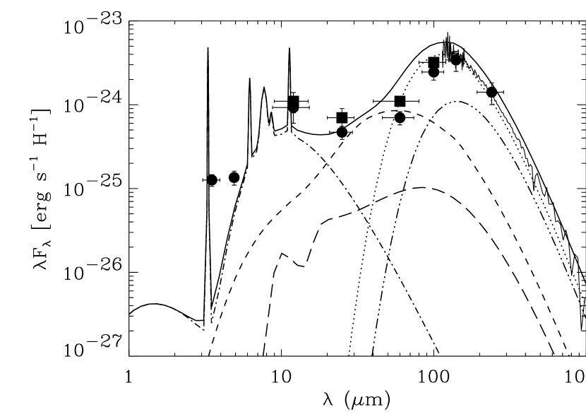
Figure 3: Predicted emission spectrum from our MW dust model exposed to the local interstellar radiation field and compared to the observed diffuse ISM spectrum. The radiation field is taken from Mathis et al. (1983). The predicted model spectrum (solid line) is decomposed into emission components from PAH molecules (dot-dash line) large ($>$100 Å) graphite and silicate grains (dotted and triple dot-dash lines, respectively) and small ($\leq$100 Å) graphite and silicate grains (short dash and long dash lines, respectively). The IRAS data (squares) are taken from Boulanger & Pérault (1988); DIRBE (circles) and FIRAS (solid line) data are taken from Dwek et al. (1997).

Table 1: Model Dust Abundances

		MW	LMC	LMC 2	SMC
	Zsi	$5.8\times 10^{-3}$	$1.9\times 10^{-3}$	$2.0\times 10^{-3}$	$1.1\times 10^{-3}$
	Zgr	$3.6\times 10^{-3}$	$7.6\times 10^{-4}$	$7.7\times 10^{-4}$	$2.4\times 10^{-4}$
Model A	ZPAH	$2.1\times 10^{-4}$	$4.8\times 10^{-5}$	$4.2\times 10^{-5}$	$9.3\times 10^{-6}$
	[C/H]	320	68	68	21
	[Si/H]	34	11	12	6
	Zsi	$5.7\times 10^{-3}$	$1.9\times 10^{-3}$	$2.1\times 10^{-3}$	$1.4\times 10^{-3}$
	ZAMC	$2.2\times 10^{-3}$	$4.2\times 10^{-4}$	$5.0\times 10^{-4}$	$1.4\times 10^{-4}$
Model B	Zgr	$8.1\times 10^{-4}$	$2.6\times 10^{-4}$	$1.8\times 10^{-4}$	$\cdots$
	ZPAH	$2.2\times 10^{-4}$	$4.7\times 10^{-5}$	$5.0\times 10^{-5}$	$1.5\times 10^{-5}$
	[C/H]	271	61	61	13
	[Si/H]	33	11	12	8

3 Dust Heating and Emission

In this section we describe the derivation of the dust emission spectrum given a dust grain model and heating sources. The determination of the emission spectrum reduces to the problem of determining the temperature dust grains of a given size and composition will reach when exposed to a radiation field. We outline the relevant equations for both equilibrium and single–photon, or transient, heating of dust grains. The actual implementation of our heating code is discussed in §3.3.

3.1 Equilibrium Heating

The monochromatic energy absorbed by a spherical dust grain of radius $a$ and species $i$ exposed to a radiation field $J_{\lambda}$ is given by

$$E^{abs}_{i}(a,\lambda)=4\pi\>\sigma_{i}(a,\lambda)\>J_{\lambda}$$ (4)

where $\sigma_{i}(a,\lambda)$ is the absorption cross section. The energy emitted by the same particle can be expressed by

$$E^{em}_{i}(a,\lambda)=4\pi\>\sigma_{i}(a,\lambda)\>B_{\lambda}(T_{i,a})$$ (5)

where $B_{\lambda}(T_{i,a})$ is the Planck function evaluated at the temperature of the grain. Thus, in a volume of space within which it is assumed $J_{\lambda}$ is constant, the equation describing the equilibrium between the energy absorbed and emitted by a single grain of radius $a$ can be written

$$\int\limits_{0}^{\infty}\!d\lambda\;\;\sigma_{i}(a,\lambda)\>J_{\lambda}=\int\limits_{0}^{\infty}\!d\lambda\;\;\sigma_{i}(a,\lambda)\>B_{\lambda}(T_{i,a}).$$ (6)

Eq. (6) can be solved iteratively for the equilibrium temperature of the dust grain. With the temperature of each individual dust grains known, the dust emission spectrum from all species and grain sizes is calculated in a straightforward manner:

$$L(\lambda)=4\pi\sum_{i}\int\limits_{a_{min}}^{a_{max}}\!da\;\;n_{i}(a)\>\sigma_{i}(a,\lambda)\>B_{\lambda}(T_{i,a}).$$ (7)

3.2 Transient Heating

The main assumption in the above discussion is that the dust grains reach equilibrium with the radiation field and can be characterized by a single temperature. While this assumption is valid for large grains, it is not generally true for small grains. The absorption of a single high energy photon by a small grain can raise its temperature significantly above its equilibrium temperature. Which grains fall into the “large” and “small” categories depends on the grain composition as well as the characteristics of the radiation field, for computational purposes the division can be roughly made at $a\simeq 100$ Å. For example, a 100 Å graphite grain at a temperature of 25 K which absorbs a Lyman limit photon ($\lambda=912$ Å) is heated to $\sim 39$ K, while a 40 Å grain will reach a temperature of $\sim 90$ K, with the temperature change becoming progressively larger for smaller and smaller grains. This temperature represents the maximum temperature the grain can reach. So while grains of all sizes will have time dependent temperatures characterized by a probability distribution, $P(T)$, rather than a single temperature, $P(T)$ will be narrowly distributed about the equilibrium temperature for large grains but small grains will have very broad temperature probability distributions. In this case, the Planck function in Eq. 7 must be replaced by an integral over the probability distribution, $P(T)$;

$$L(\lambda)=4\pi\sum_{i}\int\limits_{a_{min}}^{a_{max}}\!da\;\;n_{i}(a)\>\sigma_{i}(a,\lambda)\>\int\!dT\;\;B_{\lambda}(T_{i,a})\>P(T_{i,a}).$$ (8)

It can be seen that Eq. 7 is a special case of Eq. 8 with $P(T)=\delta(T-T_{eq})$. In determining $P(T)$, we follow the method of Guhathakurta & Draine (1989). They define a transition matrix $A_{f,i}$ whose elements are the probabilities that a grain undergoes transitions between arbitrarily chosen internal energy states $i$ and $f$. Determining $P(T)$ then amounts to solving the matrix equation

$$\sum_{i=1}^{N}A_{f,i}P_{i}=0.$$ (9)

The elements of $A_{f,i}$ are given by, in the case of heating ($f>i$)

$$A_{f,i}=4\pi\>\sigma(a,\lambda)\>J_{\lambda}\frac{hc\Delta H_{f}}{(H_{f}-H_{i})^{3}}$$ (10)

where $H_{f}$ and $H_{i}$ are the enthalpies of the final and initial states respectively and $\Delta H_{f}$ is the width of the final state. In the case of cooling ($f<i$), the elements of $A_{f,i}$ are given by

$$A_{f,i}=\left\{\begin{array}[]{rcr}\frac{4\pi}{\Delta H_{i}}\int\limits_{0}^{\infty}\!d\lambda\;\;\sigma(a,\lambda)\>B_{\lambda}(T_{i})&&i=f+1\\ 0&&\mbox{otherwise}\end{array}\right.$$ (11)

The requirement $i=f+1$ unrealistically allows cooling transitions to occur only to the next lower level. While this has little effect at short wavelengths ($<$40 µm), it can underestimate the emission from small grains at submm wavelengths (e.g., Siebenmorgen, Krugel & Mathis 1992). However, the solution of Eq. 9 without the assumption of Eq. 11 would require the inversion of a large matrix which is prohibitively expensive in computation time when incorporated in our radiative transfer code. As the long wavelength emission from dust is dominated by large grains in our application and speed is crucial, we adopt Eq. 11 and the attendant fast solution to Eq. 9 outlined by Guhathakurta & Draine (1989). Note that in the above discussion we consider only radiative processes, which are the most important for the modeling considered here. However, other sources of grain heating (e.g., electron-grain collisions) and cooling (e.g., photoelectric emission) can be modeled by additional terms in Eqs. 6, 10 & 11 (Guhathakurta & Draine, 1989).

In Figure 4, we show the grain temperature probability distributions (Eq. 9) obtained from our algorithm when the grains are placed in the Milky Way local radiation field (§2). Although the specifics of the probability distributions will vary with the radiation field, the general behaviors exhibited in Figure 4 are characteristic (e.g., Siebenmorgen et al. 1992). The smaller grains have very broad temperature distributions indicating that they have a significant probability of reaching temperatures well above and below their equilibrium temperatures. As the grain size increases, the probability distributions in a given radiation field narrow, approaching a delta function centered on their equilibrium temperatures. The width of the probability distribution is an indication of whether the grain heating can be treated as an equilibrium process (§3.3); the narrower the distribution the less important transient heating effects become.

Figure 4: Model calculations of the temperature probability distributions of silicate and graphite grains of various sizes when exposed to the local interstellar radiation field (Mathis et al., 1983).

The PAH component of our dust model (§2) will also undergo temperature fluctuations. If the cooling behavior of the molecule is known, the emission from the molecules can be calculated using time averages (Léger & Puget, 1984). The advantage of this treatment over that of Guhathakurta & Draine (1989) outlined above is an order of magnitude increase in the speed of the calculation (Siebenmorgen, Krugel & Mathis 1992). We treat the transient heating of the PAH component via time averages assuming a time dependence for the temperature of the molecule

$$T(t)=(T_{p}^{-0.4}+0.005t)^{-2.5}$$ (12)

where $T_{p}$ is the peak temperature reached by the molecule (Siebenmorgen et al., 1992). The mean time between photon absorptions is calculated from

$$\frac{1}{\overline{t}}=\frac{4\pi}{hc}\int\limits_{0}^{\lambda_{c}}\!d\lambda\>\lambda\>\sigma(a,\lambda)\>J_{\lambda}$$ (13)

where $\lambda_{c}$ is the cut-off wavelength in the optical/UV cross-section of the PAH molecule, defined by $\lambda_{c}=a/12.5$µm, when $a$ is in Å (Désert et al., 1990). The existence of a cut-off wavelength in the optical/UV cross-section of the PAH results from the discrete nature of the electronic levels in neutral PAH molecules (Désert et al., 1990). It is assumed that the molecule absorbs a single photon of wavelength

$$\lambda_{abs}=\frac{\int\limits_{0}^{\lambda_{c}}\!d\lambda\;\;\lambda\>\sigma(a,\lambda)\>J_{\lambda}}{\int\limits_{0}^{\lambda_{c}}\!d\lambda\;\;\sigma(a,\lambda)\>J_{\lambda}}$$ (14)

and cools following Eq. 12 with $T_{p}$ calculated from the enthalpy of the PAH molecule. The PAH emission spectrum is then calculated from

$$L_{PAH}(a,\lambda)=4\pi\>\sigma(a,\lambda)\>\overline{B[T(t)]}$$ (15)

where the bar indicates an average taken over the mean time between photon absorptions (Eq. 13). With the cooling behavior of the molecule approximated by Eq. 12, energy conservation is not necessarily strictly maintained and we re-normalize the emitted spectrum to ensure energy conservation (Siebenmorgen et al., 1992). Treating the PAH emission in this manner is significantly faster than the matrix method of Guhathakurta & Draine (1989) outlined above for the small carbon and silicate grains (Siebenmorgen et al., 1992).

As stated above, treating the transient heating of a grain or molecule, requires knowledge of their enthalpy (e.g., Eqs. 10,11,12). The enthalpy of the grains at temperature $T$ is defined in terms of their specific heats, $C(T)$, through

$$H(T)=\int\limits_{0}^{T}\!dT\;C(T).$$ (16)

Specific heats and enthalpies for the graphite and silicate grains were taken from Guhathakurta & Draine (1989). The enthalpy for the AMC component was assumed to be the same as that of the graphite grains. The specific heat for the PAH molecules was taken from the linear approximation of Silva et al. (1998) to the data of Léger et al. (1989).

3.3 Computational Method

In order to compute the radiative transfer and dust emission for a system, we define the spatial distributions of the gas, dust, and heating sources within an arbitrary three dimensional model space. To illustrate the dependence of the IR spectrum on various parameters, here we consider a spatial grid in the shape of a cube divided into $N^{3}$ bins. The number of model bins essentially establishes the smallest spatial scale of inhomogeneity resolved by the model, since the ratio of clump size to system radius is defined by $1/N$ (Witt & Gordon, 1996). For the models consider here, we adopt $N=30$. We consider a two-phase clumpy medium consisting of high and low density clumps, where the density of each bin is assigned randomly. The frequency of occurrence of high density clumps is determined by the filling factor ($f\!\!f$) and the relative density of high and low density model bins is characterized by the density ratio, $k=k_{2}/k_{1}$ where $k_{2}$ and $k_{1}$ are the densities of the low and high density media, respectively. In the following, we describe our computational method.

A single run of our model (where by single run we refer to a single set of input parameters, e.g., dust grain model, heating sources and their relative distribution, size, optical depth, filling factor, and density ratio) consists of the following iterative procedure:

1. Monte Carlo radiative transfer of the photons from stellar and nebular sources through the model space, resulting in the directly transmitted, scattered, and absorbed fractions of the initial input photons in each model bin.

2. Calculation of the dust emission spectrum based on the heating supplied by the fraction of the input energy absorbed in the dust and the choice of dust model.

3. Monte Carlo radiative transfer of the emitted dust spectrum through the model space, resulting in a new grid of transmitted, scattered, and absorbed fractions.

4. Convergence check. If the fractional change in the absorbed energy grid from the previous iteration is less than some tolerance (we have taken $\delta=0.01$), convergence is achieved and the run terminates. Otherwise, return to step 2 with the new absorbed energy grid.

In the following, we will describe in some detail steps 2 and 4. For a detailed discussion of the Monte Carlo radiative transfer algorithm, the reader is referred to Gordon et al. (2000).

From the Monte Carlo radiative transfer, we calculate $E_{abs,i}(\lambda)$, the total energy absorbed in each model bin. This grid of absorbed energy is passed to the dust heating algorithm. With reference to Eqs. 6 and 10, we see that we require the specific intensity of the radiation field, $J_{\lambda,i}$ in the $i^{th}$ bin in order to calculate the dust temperatures and hence the dust spectrum in that bin. In the following, we drop the subscript $i$ and implicitly assume that the calculations described are to be done in each of the $N^{3}$ bins. In order to calculate $J_{\lambda}$ from the absorbed energy, we make use of Eq. 4. Multiplying by the size distribution, integrating over grain size and summing over species, the left hand side of Eq. 4 becomes the total energy absorbed by all grain components of all sizes and we can write

$$E_{abs}(\lambda)=4\pi J_{\lambda}\overline{\sigma(\lambda)}$$ (17)

where $\overline{\sigma(\lambda)}$ is the total cross section per unit volume of the grain population:

$$\overline{\sigma(\lambda)}=\sum\int\limits_{a_{min}}^{a_{max}}\!\!da\;\frac{dn(a)}{da}\sigma(a,\lambda)$$ (18)

where the sum is over all grain components (i.e., graphite, silicates, and PAH molecules). Thus, we derive the radiation field

$$J_{\lambda}=\frac{E_{abs}(\lambda)}{4\pi\overline{\sigma(\lambda)}}.$$ (19)

With $J_{\lambda}$ known, we can proceed to deriving the temperature of each grain species and size in the equilibrium case or the temperature probability distribution in the transient case.

The heating algorithm proceeds as follows. The contribution of the PAH component to the emitted spectrum in each bin is calculated from a straightforward application of Eqs. 12–15. For the graphite and silicate grains, the calculation can be considerably more complicated. For grains with sizes $a>100$Å, we solve Eq. 6 iteratively for the temperature and the contribution of each grain size and species to the total dust spectrum in the bin is calculated via Eq. 7. For grains with sizes $a\leq 100$Å, we allow for the grain to undergo temperature fluctuations as described in §3.2. Computationally, the grain temperature must be divided into a discrete mesh. The temperature is related to the enthalpy of the grains, so selecting the temperature mesh is equivalent to defining the enthalpy mesh to be used in calculating the elements of the transition matrix, $A_{f,i}$ (Eqs. 10 & 11). Care must be taken in defining the temperature mesh; the transition matrix in Eq. 9 is $N_{T}\times N_{T}$ where $N_{T}$ is the number of temperatures in the mesh. As solving Eq. 9 is the most computationally expensive part of the code, it is advantageous to keep $N_{T}$ as small as possible. However, the probability distribution $P(T)$ must be well sampled, especially where it is changing rapidly. Hence it is crucial to select the temperature interval and $N_{T}$ carefully. We adopt an iterative approach to both the temperature interval selection as well as the number of bins. Considerable effort is made to set up the initial mesh carefully and our algorithm incorporates as much a priori information about the behavior of $P(T)$ with grain size as possible. For example, referring to Figures 4a,b, very small grains have very broad, slowly varying temperature distributions and a broad, coarse grid may be sufficient to determine $P(T)$. On the other hand, as we near the transition region between “small” and “large” grains, $P(T)$ becomes increasingly peaked near the equilibrium temperature and the broad, coarse mesh is not sufficient to sample it well. We start the algorithm by defining a relatively narrow, coarse mesh with $N_{T}=50$ equally spaced temperature intervals centered on $T_{eq}$,

$$\begin{array}[]{rclcl}0.50~{}T_{eq}\leq&T&\leq 1.50~{}T_{eq}&&T_{eq}\leq 100\\ T_{eq}-100\leq&T&\leq T_{eq}+100&&T_{eq}>100.\end{array}$$ (20)

Based on the behavior of $P(T)$ derived from Eq. 9 with this temperature grid, we adjust the upper and lower bounds of the temperature interval and the number of enthalpy bins $N_{T}$. In the case of a large grain, the coarse initial mesh will be insufficient to determine $P(T)$. The failure of the coarse mesh is manifested in a probability distribution that is highly peaked at low temperatures and zero elsewhere, i.e. it approaches one in the lowest temperature interval and zero in all other temperature intervals. In this case, we increase the number of enthalpy bins, $N_{T}$, by 50% and repeat the calculation to $P(T)$. We repeat this procedure until $P(T)$ is well behaved or we have exceeded the maximum number of enthalpy bins, $N_{T,max}$. $N_{T,max}$ is an input parameter that we have set to 800 for our model runs. In practice, $N_{T,max}$, is not exceeded in the initial set up; generally, 75 to 112 bins are sufficient to sample $P(T)$ and begin testing for convergence for even the largest grains treated by the transient heating algorithm (see below). In the case of a small grain, $P(T)$ will be a smoothly varying function across the initial narrow temperature interval and the interval needs to be expanded to insure we include the whole range of temperatures that the grain has a non-negligible probability of achieving. In this case, we expand the temperature interval to extend from $T_{min}=2.7$ K to $T_{max}=2500$ K and, keeping $N_{T}=50$, recalculate $P(T)$. This temperature interval brackets all likely temperatures that the dust grain can reach. For very small grains, this coarse, broad temperature mesh may be sufficient to begin testing for convergence. However, for intermediate sized grains, $P(T)$ may again become peaked at low temperatures and approach zero in the higher temperature bins. In this case, we define a new maximum temperature

$$T_{max}^{new}=T_{max}^{old}+0.5(T_{eq}-T_{max}^{old}).$$ (21)

$N_{T}$ is increased by 50% and a new $P(T)$ is derived with the new temperature mesh. This procedure is iterated until $P(T)$ is well behaved in the interval. In practice, one to two iterations are sufficient to roughly establish the correct temperature interval for the grain.

With the initial $P(T)$ determined as above, we calculate the predicted spectrum of the transiently heated grain using Eq. 8 and test for convergence. We define the convergence of the transient heating algorithm based on a comparison of the calculated total emitted energy and the absorbed energy,

$$\frac{\Delta E}{E_{abs}}=\frac{\left|E_{abs}-E_{em}\right|}{E_{abs}}$$ (22)

where $E_{abs}$ is calculated by integrating Eq. 4 over wavelength and $E_{em}$ is calculated from

$$E_{em}=4\pi\int\limits_{0}^{\infty}d\lambda\;\;\sigma_{i}(a,\lambda)\>\int\!dT\;\;B_{\lambda}(T_{i,a})\>P(T_{i,a}).$$ (23)

For convergence, we require that $\Delta E/E_{abs}<\delta E$, where $\delta E$ is an input parameter that we have set to 0.1 for the runs presented here. If the algorithm has not converged, we define a new temperature interval, increase $N_{T}$ by 50%, recalculate $P(T)$ and re-evaluate $\Delta E/E_{abs}$. Since there is no advantage to including temperature intervals where the grain has a very small probability of finding itself ($P(T)\ll 1$), we define a cutoff probability, $P_{cut}=10^{-15}P_{max}$, where $P_{max}$ is the maximum of the probability distribution. The new temperature interval is defined to exclude temperature bins for which $P(T)<P_{cut}$ (Manske & Henning, 1998). This procedure is iterated until convergence is achieved or we exceed $N_{T,max}$. If $N_{T,max}$ is exceeded, the grain is treated as being at its equilibrium temperature and its contribution to the spectrum is calculated with Eq. 7. The transient heating algorithm is turned off and all subsequent grain sizes are treated via the equilibrium heating formalism.

We have tested our algorithm for calculating the transient emission spectrum in a wide variety of radiation fields from the local ISRF to the radiation field in close proximity to a hot star to a variety of the SES models described above. In all cases the algorithm worked with no user interaction and produced probability distributions with the correct behavior as a function of grain size and radiation field (e.g., see Figs. 4a,b). In addition, we have compared the results from our algorithm with previous calculations in the literature (Siebenmorgen et al., 1992; Manske & Henning, 1998) with excellent agreement. In light of these tests, we are confident that we can apply our model to a range of situations with minimal adjustments to the heating calculation.

A single run of the dust heating algorithm is complete when the above procedure has been performed for all model bins for which the absorbed energy in that bin exceeds some cutoff fraction. The cutoff fraction is determined as follows. In each bin we calculate the fraction of the total energy absorbed,

$$f_{abs,i}=\frac{E_{abs,i}}{\sum_{i}E_{abs,i}}.$$ (24)

We then calculate the quantity $\sum_{i}f_{abs,i}$ for $f_{abs,i}>f_{cut}$ for a variety of values of $f_{cut}$. We adopt a value of $f_{cut}$ such that the total energy absorbed in bins for which $f_{abs,i}>f_{cut}$ is larger than some target level of energy conservation. The target level is taken as an input and is generally between 0.95 and 1. This level represents the best possible energy conservation that can be achieved for the run; model bins with $f_{abs,i}<f_{cut}$ are not included in the dust heating algorithm. This procedure allows us to eliminate a large number of model bins in which very little energy is absorbed, speeding up the calculation substantially with little cost in accuracy.

Upon completing a single run of the dust heating algorithm, we obtain the dust emission spectrum from each point in the model. In order to allow for the treatment of large optical depths and to account for the dust self–absorption, we now add the dust as a new source of emitted photons. The Monte Carlo radiative transfer code is re–run, now using the dust spectrum as the source of input photons rather than the stellar and nebular sources. The contribution of the dust emission to the absorbed energy in each model bin as derived from the Monte Carlo is then added back into the absorbed energy grid from the previous iteration, and the fractional change in the total absorbed energy is computed. We consider the entire model run to have converged if the fractional change in absorbed energy $\delta<0.01$. If $\delta\geq 0.01$, the new absorbed energy grid is passed to the dust heating algorithm and steps 2–4 are repeated. When convergence is achieved in step 4, a single model run has been completed. In general, even for large optical depths (e.g., $\tau_{V}=20-50$), convergence is achieved in fewer than 4 full iterations of steps 2–4. For optical depths in the range of $\tau_{V}=2-10$, 2 iterations are normally sufficient to reach convergence.

In addition to the far-UV to far-IR SED of the model, several other quantities are included in the output upon the completion of a model run, including the size averaged dust temperature for each dust component in each model bin, the relative fractions of the total energy absorbed in the clump vs. interclump medium, and the total dust mass of the model. We define the size averaged dust temperature for each dust component in the following way;

$$\overline{T}_{i}=\frac{\int\limits_{a_{min}}^{a_{max}}\!da\;\;n_{i}(a)T_{i}(a)}{\int\limits_{a_{min}}^{a_{max}}\!da\;\;n_{i}(a)}.$$ (25)

Note that in Eq. 25, $T_{i}$ is the equilibrium temperature of the grain and hence the size averaged temperature does not account for the range of temperatures reached by stochastically heated grains. Since we have the temperature in each bin, $\overline{T}$ may be used to calculate the radial temperature distribution of the dust in the model (see §4).

We calculate the total dust mass in each model in the following way:

$$M_{dust}=\sum_{i}^{N_{bins}}\frac{N_{H,i}}{\tau_{V,i}}\left[\tilde{\tau}_{V,i}V_{i}\sum_{j}\int\limits_{a_{min}}^{a_{max}}\!\!da\;\frac{4\pi}{3}a^{3}\rho_{j}n_{j}(a)\right]$$ (26)

where the sum over $i$ is taken over model bins, $\tilde{\tau}_{V,i}$ is the optical depth per unit $pc$ at $V$ in the $i^{th}$ bin and $V_{i}$ is the volume of the $i^{th}$ bin in $pc^{3}$. The term in brackets gives the dust mass per hydrogen column times $\tau_{V,i}$, where the sum over $j$ is over dust components. In order to calculate the total dust mass we assume a gas to dust ratio and a value of the ratio of total to selective extinction, $R_{V}$. For each of the four dust models considered (see §2), we take $R_{V}$ = 3.1 and a gas to dust ratio ($N_{H}/E(B-V))$of $5.8\times 10^{21}$, $2.4\times 10^{22}$, and $5.0\times 10^{22}~{}~{}$ H atoms/cm²/mag^-1 for the MW, both LMC models, and the SMC, respectively.

4 An Example: Starburst Galaxies

The DIRTY  model is completely general in that we can treat arbitrary distributions of dust and heating sources. However, to illustrate how the model predictions depend on various input parameters, here we apply DIRTY  to input stellar distributions and geometric environments appropriate for the modeling of starburst galaxies (Gordon et al., 1997; Witt & Gordon, 2000). Witt & Gordon (2000) defined different star/dust geometries including DUSTY and SHELL geometries. The DUSTY geometry contains dust and stars mixed together, with both extending to the system radius. The SHELL geometry consists of stars extending to 0.3 of the system radius with dust filling a shell extending from 0.3 to the system radius. Pictorial representations of these geometries can be found in Fig. 1 of Witt & Gordon (2000). We emphasize that the DUSTY and SHELL geometries specify the global geometry of the model space; locally, each model bin can be either clumpy or homogeneous, as characterized by the $f\!\!f$ and the density ratio $k_{2}/k_{1}$. While the model is capable of handling any arbitrary geometry, these two geometries are expected to be representative of a wide range of star/dust geometries, e.g., embedded stellar populations and mixed stars and dust.

Within the global geometries described above, MW, LMC, or SMC type dust (§2) is distributed with a local geometry determined by the $f\!\!f$ and density ratio. The stellar population is distributed uniformly within the global geometries. The properties of the stellar population are taken from the stellar evolutionary synthesis models of Fioc & Rocca-Volmerange (1997, 2000; http://www.iap.fr/users/fioc/PEGASE.html) (PEGASE models). The starburst models presented here were run using an IMF with a mass range of $0.1-100M_{\sun}$ with a Salpeter slope, a constant star formation scenario, ages ranging from $0-19$ Gyr, with a range of metallicities from $-$2.3 to 0.7, and include a nebular component. For a more detailed discussion of the spectral synthesis model in the context of the DIRTY  model, the reader is referred to Gordon et al. (1999). The input stellar SEDs are rebinned to $\sim 120$ wavelength points. The model SEDs for young input stellar populations exhibit features near 0.37 and 0.67 µm resulting from contributions to the rebinned SED from strong nebular emission lines (O II and H$\alpha$, N II) in those wavelength regions.

In the following discussion, we present the results of several sets of DIRTY  model runs using the starburst stellar distributions and geometries described above. We examine the dependence of the spectrum, dust temperatures, and dust masses on variations in the input parameters. The input parameters for DIRTY  include: metallicity, star formation rate, and age, which together determine the spectral shape and intensity of the input SED; the filling factor ($f\!\!f$) and density ratio ($k=k_{2}/k_{1}$), which determine the clumpiness of the scattering and absorbing dusty medium; the dust type which determines the composition and size distribution of the dust grains; and the physical size of the region, the global geometry, and the optical depth, $\tau_{V}$, which affect the dust mass as well as the efficiency of a given mass of dust in absorbing the photons from the input SED. The input optical depth, $\tau_{V}$, for both DUSTY and SHELL geometries is defined as the radial optical depth, from the center to the edge of the model, that would result were the dusty medium distributed homogeneously throughout the model space. The range of values for these parameters is tabulated in Table 2. The case of the application of DIRTY  to starburst galaxies will be considered in more detail in a forthcoming paper; in the following, we adopt dust Model A for illustrative purposes.

Table 2: Input Model Parameters

Parameter	Range	Figure Reference	Fixed Value
Metallicity	-0.4	$\cdots$	$\cdots$
Dust Type	MW,SMC	5,7(a)	$\cdots$
Dust Model	A,B	7(b)	A
Global Geometry	SHELL,DUSTY	9, 10, 11, 14	$\cdots$
$f\!\!f$ (filling factor)	0.05 – 0.5	6	0.15
$k$ (density ratio)	0.001 – 0.177	6	0.01
SFR	0.5 – 200 M⊙ yr-1	16,17	1.6 M⊙ yr-1
Age	$10^{6}$ – $19\times 10^{9}$ yr	16,17	40 Myr
Size	10 – 5000 pc	13	1000 pc
$\tau_{V}$	0.5 – 20.0	9, 10, 11, 14	10

4.1 Transient Heating

In Figure 5, we illustrate the effects of including the transient heating (see §3.2) of small grains and molecules on the SEDs predicted by our starburst model. Including the effects of transient heating in the model increases the predicted emission between $5-30$ µm by as much as a factor of 20 for the cases presented in Figure 5.

Figure 5: Model SED’s for MW and SMC type dust models with and without the effects of transient heating of the small grains. The equilibrium cases include neither the effects of transient heating nor the emission from small grains nor a molecular (PAH) component, the non equilibrium cases include both. All parameters are set to their values in column 4 of Table 2 and a SHELL geometry is assumed.

4.2 Clumpiness

In this section, we illustrate the dependence of the predicted SED on the local structure of the absorbing medium. The local structure is characterized by $f\!\!f$ and $k$, and we keep all other model inputs fixed at their values listed in column 4 of Table 2, assuming a SHELL geometry and a model size of 30 bins per side. We have considered $f\!\!f$’s between $0.05$ and $0.5$, with a range of physical conditions varying from an extended low density medium with rare, isolated high density clumps to an interconnected network of high density clumps with a low density medium filling the voids. The value of $k$ is varied between $0.001$ and $1$ (homogeneous) in steps of factors of $\sim$5.62 ($k=0.001,0.005,0.030,0.177,1.0$). The effect of varying $f\!\!f$ and $k$ on the SED is illustrated in Figs. 6a,b,c,d. We do not include the homogeneous case in the Figures as the change in the SED between $k=0.177$ and $1$ is negligible for all values of $f\!\!f$. For all values of $f\!\!f$, the effect of increasing $k$ on the IR SED is to shift the peak of the dust emission to shorter wavelengths, corresponding to higher dust temperatures. The effect is quite small and becomes less pronounced with increasing $f\!\!f$ and for $f\!\!f>0.20$, the IR SED’s are essentially degenerate for different values of $k$. The dominant reason for this behavior is the increase in total energy absorbed by the dust with increasing $k$ at a constant $f\!\!f$ which results in more heating and higher dust temperatures. A smaller secondary contribution to the behavior results from the fact that at higher values of $k$, a correspondingly larger fraction of the energy is absorbed in the low density medium which reaches higher temperatures than the dense clumps. In any case, as can be seen from Fig. 6, the model IR SED is not very sensitive to the local structure of the medium. The dominant effects of $f\!\!f$ and $k$ are seen in the optical and UV SED (Witt & Gordon, 1996).

Figure 6: Model SED’s for a range of density ratios ($k=0.001$ solid line, $k=0.005$ dashed line, $k=0.03$ dash-dot line, $k=0.177$ dash-triple dot line) with different filling factors; (a) $f\!\!f=0.05$, (b) $f\!\!f=0.1$, (c) $f\!\!f=0.2$, (d) $f\!\!f=0.5$. All models are calculated assuming SHELL geometry, 30 bins per side, and the remaining parameters specified in column 4 of Table 2.

4.3 Dust Type (MW vs SMC) & Dust Model (A vs B)

Observations of UV extinction along different lines of sight in the local group of galaxies (e.g., mainly the MW, LMC, and SMC) have revealed a range of characteristic extinction curves which can be broadly associated with the galaxy being observed, although variations along different lines of sight within a given galaxy can be substantial (e.g., Cardelli et al., 1989; Gordon & Clayton, 1999; Misselt et al., 1999; Clayton et al., 2000b). For illustrative purposes, in this paper we concentrate on MW and SMC type dust. The MW type dust extinction is characterized in the UV by the 2175 Å bump and rising far UV extinction. On the other hand, the UV extinction in the SMC is conspicuous in the absence of the 2175 Å feature. In addition, the far UV rise in the SMC extinction curve is nearly linear with $\lambda^{-1}$ and is steeper than in the MW. As discussed in §2, these extinction curve characteristics are reproduced in our model by varying the grain size distributions and the relative contributions of the various grain components to the extinction curve. Hence, the steepness of the far UV extinction in the SMC and the absence of the 2175 Å feature require a larger number of small silicate grains and fewer small graphite grains, respectively, in the SMC dust model compared to the MW. In Figure 7(a), the difference between utilizing MW and SMC type dust in our model is illustrated. The difference is manifested in the UV SED in the presence of an absorption feature near 0.22 $\micron$ in the SED derived using MW type dust and an increase in the far UV absorption in the SED derived using SMC type dust. There are also pronounced differences in the predicted IR SED depending on the dust model used. A subtle difference is seen in the depth of the $\sim 9.7~{}\micron$ absorption feature, which is deeper in the SMC SED compared to the MW curve. Since the $9.7~{}\micron$ feature is attributed to stretching and bending resonances in the small silicate grains (Whittet, 1992), its strength in the SMC SED is not surprising given that a large number of small silicate grains are required in the SMC dust model to reproduce the steep linear rise in the far UV extinction curve. The most apparent difference is the excess in mid IR emission present in the MW SED as compared to the SMC. This is easily understood in terms of the larger populations of small, graphitic grains and PAH molecules in the MW type dust model. These grain populations dominate the emission from grains undergoing transient heating (§3.2) and hence there are more small grains at high temperatures when the MW dust model is used resulting in increased emission in the mid IR. The mid IR emission from the SMC type dust can be enhanced by utilizing dust Model B (see 7(b)). The low mid IR emission from the SMC type dust using dust Model A results from the paucity of small carbonaceous grains. By introducing a population of small carbonaceous grains in the form of AMC, the importance of transient heating is amplified without introducing a 2175 Å absorption feature in the resulting extinction curve.

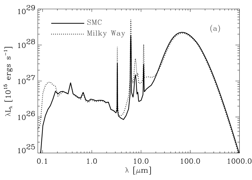
Figure 7: Comparison of the effects of using different grain models (§2) on the predicted starburst SED. (a) Comparison of MW and SMC type dust using grain model A. (b) Comparison of SMC type dust using grain models A & B. All SEDs calculated for same set of input parameters (see Table 2, column 4) save the dust type and grain model.

Observationally, a substantial population of small grains undergoing temperature fluctuations would be manifested in higher mid IR fluxes than expected from large grains in equilibrium. Indeed, ground based observations (Andriesse, 1978; Sellgren, Werner & Dinerstein, 1983; Sellgren, 1984; Sellgren et al., 1985) along with early results from the IRAS satellite (e.g., Boulanger et. al. 1988; Boulanger & Pérault 1988 and references therein) of significant emission in the mid IR in a variety of environments were a large driving force in the development of ways to treat the heating of small grains and the recognition that small grains must be a significant component of interstellar dust (Léger & Puget, 1984; Draine & Anderson, 1985; Dwek, 1986). The effect of increased emission in the mid IR on, for example, IRAS colors, is to increase the F${}_{\lambda}(12\micron)$/F${}_{\lambda}(25\micron)$ and F${}_{\lambda}(25\micron)$/F${}_{\lambda}(60\micron)$ flux ratios. As we are illustrating the behavior of the DIRTY  model in the context of a starburst galaxy model in this paper, in Figures 8a–c, we plot the IRAS colors of starburst galaxies with measured fluxes in all four IRAS bands from the sample of Gordon et al. (1997), along with tracks from runs of the DIRTY  model. Runs are included for a range of optical depths, physical sizes, star formation rates, geometries, and all were run using dust Model A. Model data points were determined by convolving model SEDs with the response functions of the IRAS bandpasses as tabulated in the online IRAS Explanatory Supplement.

The first thing to notice is that the model results cover essentially the full range of observed starburst colors. However, in detail, the model colors show some discrepancies compared to observations, as is especially evident in Figures 8b & c. The discrepancy between the model colors and the starburst data is attributable to low mid IR fluxes predicted by the former, especially at 25 µm. The low predicted mid IR fluxes can be traced directly to the dust model. As can be seen in Figures 8b & c, the discrepancy between DIRTY  colors and the data is lessened when the MW dust model is used. This results from the inclusion of more small graphite grains and PAH molecules in the MW dust model (§2), which increases the contribution of transient heating to the mid IR emission (see §4.1 and Figures 5 & 7). While it is not our intention with this paper to explore in detail the wide range of systems to which the DIRTY  model can be applied, including starbursts, these figures are indicative of the diagnostic potential of properly done, self–consistent UV to far IR radiative transfer simulations. The apparent deficit of small grains could be alleviated by including a separate, large population of small graphitic grains in the dust model. However, the absence of a significant 2175 Å absorption feature in the UV SEDs of many starburst galaxies (Gordon et al., 1997) makes such a modification of the grain model problematic as the small graphite grains are responsible for this feature in our dust model. Hence, self–consistently reproducing the SEDs of starburst galaxies over a wide wavelength regime may require more complicated grain models, such as a four component model including amorphous carbonaceous grains in addition to the PAH, graphite and silicates (i.e., dust grain model B). Indeed, using our dust grain Model B with a size distribution appropriate for the SMC brings the colors of the predicted SED into better agreement with the observed colors (see Figure 7(b)). Such a diagnostic of grain materials may provide insight into grain processing histories and grain evolution in response to a wide range of environmental factors (e.g. Gordon & Clayton, 1998; Misselt et al., 1999; Clayton et al., 2000a,b). Alternatively, in the case of starbursts, the simplistic assumptions of a single stellar population and relatively simple global geometries in the models discussed above will likely need to be modified and more complicated arrangements considered.

Figure 8: IRAS color–color plot for starburst galaxies with various model runs superposed. The crosses are IRAS data for starburst galaxies from Gordon et al. (1997) with data in all four IRAS bands. Dashed and solid lines represent models using MW and SMC type dust respectively. A sequence of varying physical size models (100, 500, 1000, & 5000 pc) is indicated with filled circles. The open circles represent a series of models with varying optical depths with $\tau_{V}$=0.5,1.0,10,20. Sequences of varying SFR models are shown with open diamonds for a DUSTY global geometry & filled diamonds for a SHELL global geometry. Star formation rates along the sequences are 1, 10, 50, & 100 M_⊙ yr^-1. All parameters not varying along a sequence are kept fixed at the values indicated in column 4 of Table 2.

4.4 Global Geometry, $\tau_{V}$, & Physical Size

Figure 9 contrasts the behavior of the SHELL and DUSTY geometries at the same optical depth. We plot the model SEDs for both geometries for two extreme optical depths, $\tau_{V}=1$ and $20$ with all other input parameters set to the values in column 4 of Table 2. At a given $\tau_{V}$, the SHELL geometry absorbs more energy than the DUSTY geometry since in the SHELL configuration the stars lie inside all the dust while in the DUSTY configuration the stars are mixed throughout the dust so energy from stars in the outer parts of the model has a greater chance of escaping the model space without being absorbed (Witt & Gordon, 2000). As a result, at a given optical depth, the IR emission from the SHELL geometry will always peak at shorter wavelengths. In addition, owing to the temperature structure, the SHELL geometry produces a broader IR SED. While the dust near the centrally distributed heating sources reaches higher temperatures in the SHELL geometry, dust in the outlying regions sees fewer high energy photons and subsequently is heated to lower temperatures. Since heating sources are distributed throughout the model with the DUSTY geometry, the resulting temperature distribution is much flatter than in the SHELL case (see Fig 10a,b), resulting in a narrower IR SED.

Figure 9: Direct comparison of SHELL and DUSTY geometries at $\tau_{V}=1$ and $\tau_{V}=20$. All other input parameters are fixed at the values in column 4 of Table 2.

Figure 10: Comparison of the radial dust temperature (Eq. 25) distribution of graphite grains in SHELL and DUSTY geometries for (a) $\tau_{V}=1$ and (b) $\tau_{V}=20$. All other input parameters are fixed at the values in column 4 of Table 2 in both figures.

For a given physical model size, specifying the input optical depth, $\tau_{V}$, is equivalent to specifying the dust mass. The input optical depth is defined as the radial optical depth that would result were the dusty medium distributed homogeneously in the model space. For a clumpy dust distribution, the optical depth along a given line of sight may have a range of values from a small fraction of $\tau_{V}$ to several times larger, depending on $f\!\!f$ and $k$, and the effective optical depth will be significantly reduced with respect to the homogeneous case (Witt & Gordon, 1996, 2000).

In Figures 9 & 11a,b, we show the effects of varying $\tau_{V}$ on the predicted SED with all other input parameters kept constant. Figures 11a & 11b show a series of model calculations with increasing $\tau_{V}$ for SHELL and DUSTY geometries, respectively. In both cases, as $\tau_{V}$ increases, the IR SED broadens and the peak of the IR emission shifts to longer wavelengths. The shift to longer wavelengths, corresponding to lower dust temperatures, is a result of higher dust masses with increasing $\tau_{V}$. So even though more of the input energy is absorbed as $\tau_{V}$ increases, there is more dust to heat and the dust is consequently cooler. The IR SED broadens as a result of the increasing importance of the lower density medium in absorbing the input energy. For a constant $f\!\!f$ and $k$, as $\tau_{V}$ increases, the fraction of energy absorbed in the low density medium increases. Since the low density medium reaches higher temperatures than the dense clumps, there is a wider range of dust temperatures for high $\tau_{V}$ as compared to the low $\tau_{V}$ models where most of the energy is absorbed in the dense clumps (see Figure 12). In addition, at high $\tau_{V}$, the opacity of the dust is still significant even at mid IR wavelengths and some of the energy emitted by the dust is re-absorbed and emitted at longer wavelengths, further broadening the IR SED.

Figure 11: Dependence of the model SED on variations in the input optical depth, $\tau_{V}$, for (a) SHELL and (b) DUSTY global geometries. All other input parameters are fixed at the values in column 4 of Table 2.

Figure 12: Size averaged equilibrium dust temperature (Eq. 25) as a function of radial position. Temperatures in the low and high density model bins are plotted for two values of the input optical depth. For clarity, only the temperatures for the graphite grains are shown; results for the silicate grain component are similar. All other input parameters are fixed at the values in column 4 of Table 2.

Along with $\tau_{V}$, the physical size of the modeled region will determine the total dust mass of the system and hence affect the predicted IR spectrum from the dust emission. There is no dependence in the optical to UV spectrum on the system size since the radiative transfer (and hence total energy absorbed at any point in the model) depends only on the total optical depth through a given model bin. On the other hand, the dust mass in a given model bin depends not only on the optical depth, but also the physical size of the bin; the larger the bin, the higher the dust mass (see Eq. 26). As the temperature an individual dust grain will reach depends on the ratio of the energy absorbed to the total dust mass, increasing the size of the model (and hence the size and dust mass of the individual model bins) results in a decrease in the temperature of individual grains. Therefore, we expect the peak of the infrared emission to shift to longer wavelengths as we increase the size of the model. We see exactly this dependence in Figures 13a,b where we plot the predicted SED for a range of model radii from 100 pc to 5000 pc for both (a) SMC and (b) MW type dust models. The peak of the IR dust spectrum shifts from $\sim 45$µm to $\sim$200µm over the range of sizes considered. Of particular importance is the fact that, although the peak shifts to longer wavelengths, the spectrum is not what would be observed by simply shifting the smaller radius model SED to longer wavelengths. The larger models still exhibit substantial IR emission at shorter wavelengths from $\sim$10 µm to $\sim$50 µm, illustrating the importance of the inclusion of small, transiently heated grains in the model. The transient heating of the small grains does not depend on the total energy absorbed. While the equilibrium heating of the dust results in lower dust temperatures, the temperature excursions experienced by the small grains (§3.2) result in a contribution to IR SED at shorter wavelengths, characteristic of hotter dust grains. The same behavior is seen for both dust type models with the only difference being the higher mid–IR emission from the MW type dust resulting from a larger contribution from small graphite grains to the SED (§4.3).

Figure 13: Variation of the model SEDs for a range of model sizes for an assumed (a) SMC and (b) MW dust model. All other input parameters are fixed at the values in column 4 of Table 2.

The input parameters that determine the dust mass in a given model are the physical size, $\tau_{V}$, the dust grain model (MW, LMC, SMC), and the global geometry. The clumpiness of the local dust distribution leads to statistical fluctuations in the total mass, but on average the mass of models with different $f\!\!f$ and $k$ remains the same (Witt & Gordon, 1996). The remaining input parameters pertain to the input stellar population and do not affect the dust mass. In Figure 14, we plot the dependence of the total model dust mass on (a) $\tau_{V}$ and (b) physical size for the SHELL and DUSTY geometries.

Figure 14: Dependence of the total model dust mass on (a) the physical size and (b) $\tau_{V}$ for both DUSTY and SHELL geometries. In (a) $\tau_{V}$ is kept constant at 10 while in (b), the physical size is kept constant at 1000 pc. All other model parameters are fixed at the values in Column 4 of Table 2.

4.5 Age and Star Formation Rate

The application of the DIRTY  model to starburst galaxies requires the specification of the stellar content of the galaxy along with its star formation history. In general, the star formation history can be characterized by either a burst scenario, wherein all the stars form at once and subsequently evolve, or by a constant star formation scenario, wherein stars form continuously as the starburst ages. While the situation in real starburst galaxies is likely somewhere in between, for the purpose of illustrating the DIRTY  model, we consider only the constant star formation scenario. For this scenario, an increase in either age or star formation rates will lead to an increase in the total mass of the starburst. Increasing the age of the starburst while keeping the SFR constant, while increasing the total stellar mass, results in an increase of the importance of the contribution of older, less luminous stars to the SED relative to the hot, young stars which dominate the UV. As the starburst ages, the massive young stars are continuously replenished and their contribution to the UV SED approaches a constant as an equilibrium is reached between their formation and evolution. Hence, increasing the mass of the starburst by increasing its age results in a higher and higher fraction of its energy being produced in the optical and NIR wavelength regime. The result is a change in the shape of the input SED as the starburst ages, the UV approaching a constant with the optical and NIR increasing in importance; see Figure 15. On the other hand, increasing the mass of the starburst by increasing the SFR at a constant age has the effect of simply scaling up the input SED. At a given age, increasing the SFR results in an increase in the number of old and young stars and the total emitted energy increases at all wavelengths. The effects of these variations in the shape and total luminosity of the input SED on the predicted IR dust emission spectrum are illustrated in Figures 16a, 16b, and 17.

Figure 15: Sample input SEDs from the PEGASE synthesis models (Fioc & Rocca-Volmerange, 1997, 2000), for increasing age at a constant SFR of 1 M_⊙ yr^-1. The total mass of the starburst is increasing from bottom to top.

As is seen in Figure 16b, increasing the SFR rate at a constant age results in a shift of the peak of the IR emission to shorter wavelengths. Since the shape of the input SED does not change, but only the total amount of input energy, the dust absorbs the same fraction of the total energy ($\sim$97% for the cases plotted here) and the absorbed energy is distributed between the high and low density clumps in the same fractions as well. The result is that as the total amount of input energy is increased, all of the dust is heated to higher temperatures and the IR emission increases and its peak shifts to shorter wavelengths. Similarly, in the case of increasing age, the total IR emission from dust increases and the peak of the IR emission also shifts to shorter wavelengths. However, the effects are much less pronounced (Figure 16a). The reason for the smaller effect is three-fold. (1) Since the stellar population is aging, the same mass of stars produces less energy compared to a young, high SFR burst. Therefore, increasing the mass of the starburst by increasing its age results in a much smaller increase in the energy available for absorption in the dust as compared to increasing the mass by the same amount by increasing the SFR. (2) The input SED has changed shape so there is a larger contribution to the total input energy at optical and NIR wavelengths, resulting in less efficient dust absorption since the efficiency of dust at absorbing and scattering radiation decreases with increasing wavelength. As a result, energy is less likely to be absorbed and the fraction of the total energy absorbed by the dust falls from $\sim$97% to $\sim$83% for the cases plotted in Figure 16a. (3) Also as a result of the decreasing efficiency of dust absorption, a higher fraction of the total energy is absorbed in high density bins with increasing starburst age. Since the low density medium is heated to a higher temperature for a given input energy, the shift to increasing importance of the high density clumps results in a smaller overall temperature increase, and hence less of a shift in the peak of the dust emission to shorter wavelengths, than would be the case if the relative fraction of energy absorbed in the high and low density media remained constant. For the cases plotted in Figure 16a, the fraction of the energy absorbed in the high density clumps increases from $\sim$68% to $\sim$82% for the starburst ages considered.

Figure 16: Variation of the predicted SED with (a) increasing starburst age for constant SFR of 1.6 M_⊙ yr^-1 and (b) increasing SFR at a constant burst age of 40 Myr. All other input model parameters are kept fixed at the values given in column 4 of Table 2.

The difference between the constant SFR rate and the constant age models is illustrated in Figure 17. The solid line represents the SED of a model with a total stellar mass of $6.4\times 10^{7}$ M_⊙ (SFR=1.6 M_⊙ yr^-1, age=40 Myr). We increase the mass of the model to $8\times 10^{9}$ M_⊙ by increasing the SFR to 200 M_⊙ yr^-1 keeping the age constant (dashed line) and by keeping the SFR constant and increasing the age to 5 Gyr (dotted line). Increasing the age increases the total dust emission by a small fraction and shifts the peak wavelength of the dust emission slightly to shorter wavelengths. On the other hand, increasing the SFR dramatically increases the total dust emission and shifts the peak wavelength significantly.

Figure 17: Comparison of predicted model SEDs with same total stellar mass. Solid line, total stellar mass of $6.4\times 10^{7}$ M_⊙ with SFR=1.6 M_⊙ yr^-1, age=40 Myr. The dotted line SED results from increasing the total stellar mass to $8\times 10^{9}$ M_⊙ by increasing the starburst age to 5 Gyr while keeping the SFR constant at 1.6 M_⊙ yr^-1. The dashed line SED is the result of increasing the total stellar mass to $8\times 10^{9}$ M_⊙ by increasing the SFR to 200 M_⊙ yr^-1 while keeping the age constant at 40 Myr. All other input model parameters are kept fixed at the values given in column 4 of Table 2.

5 Conclusion and Summary

In this paper and a companion paper (Gordon et al., 2000), we have presented the DIRTY  model, a self-consistent Monte Carlo radiative transfer and dust emission model. The strengths of DIRTY  include:

• Self-consistency. No ad hoc assumptions about the dust temperature are made; the dust is heated by the absorption of photons originating from sources included in the model. The temperature distribution of the dust grains, and hence their emission spectrum, is calculated self-consistently by keeping track of the energy absorbed by dust in the Monte Carlo radiative transfer.

• Treatment of the heating of and emission from small grains, including the effects of temperature fluctuations resulting from the absorption of single photons.

• The ability to properly treat high optical depth situations. The iterative solution outlined above, wherein dust self-absorption is considered, permits the treatment of high optical depth cases, where the optically thin assumption may be violated even at IR wavelengths.

• Properly including the FIR emission from dust in DIRTY  provides additional information regarding the dust model, the nature of the heating source(s), and the physical size of the modeled region, not available through UV–NIR modeling alone.

• The use of Monte Carlo techniques to solve the radiative transfer equations allows the treatment of arbitrary dust and heating source distributions as well as inhomogeneous dust distributions (clumpiness). Though we have concentrated on starburst galaxies in exploring the parameter space of DIRTY  , it is of general applicability and can be used to model e.g., dust tori in AGNs and Quasars, circumstellar discs, individual star forming regions, and reflection nebulae.

To emphasize this last point, we point out that the fits to any UV–NIR SED are degenerate; there are in general several possible combinations of geometries, dust models and heating sources which can provide essentially identical fits to the SED. However, by examining the IR dust spectrum (total energy emitted by dust, peak wavelength of the IR emission, the strength of the mid IR emission relative to longer IR wavelengths, and strength of IR absorption and emission features), some of the degeneracy in the UV–NIR models can be lifted. Indeed, the FIR dust spectrum provides information on the physical size of the region not accessible to UV–NIR modeling alone.

Future papers will detail the application of DIRTY  to interpreting observations of astrophysical systems including individual starburst galaxies. Improvements to the current model are also being implemented. We have presented a fairly simple treatment of the PAH component here; we have not included a means of varying the relative strengths of the PAH features. Since the strengths of some of the features depend on the number of hydrogen atoms in the molecule, while others depend on the number of carbon atoms, the relative strengths can be varied by adjusting the hydrogen coverage, $x_{H}$ (see §2). Applications to specific, individual objects will require this sort of fine tuning as the relative strengths of the MIR emission features are observed to change from object to object and environment to environment (Cohen et al., 1989). A major area of effort will be in applying DIRTY  in a starburst model that will include multiple stellar populations and evolutionary effects. This will require the inclusion of the effects of the interaction between on-going star formation and dust, including the evolution of the grains due to processing, formation, and destruction (e.g. Efstathiou, Rowan-Robinson & Siebenmorgen 2000).

References

- Acosta-Pulido et al. (1996) Acosta-Pulido, J. A. et al. 1996 A&A, 315, L121
- Allamandola et al. (1989) Allamandola, L. J., Tielens, A. G. G. M., & Barker, J. R. 1989, ApJS, 71, 733
- Andriesse (1978) Andriesse, C. D. 1978, A&A, 66, 169
- Bianchi et al. (1996) Bianchi, L., Clayton, G. C., Bohlin, R. C., Hutchings, J. B., & Massey, P. 1996, ApJ, 471, 203
- Bohren & Huffman (1983) Bohren, C. F., & Huffman, D. R. 1983, Absorption and Scattering of Light by Small Particles, (New York:John Wiley & Sons)
- Boulanger et al. (1988) Boulanger, F., Beichman, C., Désert, F. X., Helou, G., Pérault, M., & Ryter, C. 1988, ApJ, 332, 328
- Boulanger & Pérault (1988) Boulanger, F., & Pérault, M. 1988, ApJ, 330, 964
- Cardelli et al. (1989) Cardelli, J., Clayton, G. C., & Mathis, J. 1989, ApJ, 345, 245 (CCM)
- Clayton et al. (2000a) Clayton, G. C., Wolff, M. J., Gordon, K. D., & Misselt, K. A. 2000a, in ASP Conf. Ser. Vol. 196, Thermal emission Spectroscopy and Analysis of Dust, Disks, and Regoliths, ed. M. L. Sitko, A. L. Sprague, & D. K. Lynch (San Francisco: ASP), 41
- Clayton et al. (2000b) Clatyon, G. C., Gordon, K. D., & Wolff, M. J. 2000b, ApJS, In Press (Aug. 2000)
- Cohen et al. (1989) Cohen, M. et al. 1989, ApJ, 341, 246
- Désert et al. (1990) Désert, F.-X., Boulanger, F., & Puget, J. L. 1990, A&A, 237, 215
- Draine & Anderson (1985) Draine, B. T., & Anderson, N. 1985, ApJ, 292, 494
- Dudley & Wynn-Williams (1997) Dudley, C. C., & Wynn-Williams, C. G. 1997, ApJ, 488, 720
- Duley (1989) Duley, W. W. 1989, in IAU Symp. 135, Interstellar Dust, ed. L. J. Allamandola, & A. G. G. M. Tielens (Dordrecht:Kluwer Academic Publishers), 141
- Dwek (1986) Dwek, E. 1986, ApJ, 302, 363
- Dwek et al. (1997) Dwek, E. et al. 1997, ApJ, 475, 565
- Efstathiou & Rowan-Robinson (1995) Efstathiou, A., & Rowan-Robinson, M. MNRAS, 273, 649
- Efstathiou et al. (2000) Efstathiou, A., Rowan-Robinson, M., & Siebenmorgen, R. 2000, MNRAS, 313, 734
- Fioc & Rocca-Volmerange (1997) Fioc, M., & Rocca-Volmerange, B. 1997, A&A, 326, 950
- Fioc & Rocca-Volmerange (2000) Fioc, M., & Rocca-Volmerange, B. 2000, in preparation
- Gordon et al. (1997) Gordon, K. D., Calzetti, D., & Witt, A. N. 1997, ApJ, 487, 625
- Gordon & Clayton (1998) Gordon, K. D., & Clayton, G. C. 1998, ApJ, 500, 816
- Gordon et al. (1999) Gordon, K. D., Hanson, M. M., Clayton, G. C., Rieke, G. H., & Misselt, K. A. 1999, ApJ, 519, 165
- Gordon et al. (2000) Gordon, K. D., Misselt, K. A., Witt, A. N., Clayton, G. C., & Wolff, M. J. 2000, in preparation
- Guhathakurta & Draine (1989) Guhathakurta, P., & Draine, B. T. 1989, ApJ, 345, 230
- Heckman et al. (1998) Heckman, T. M., Robert, C., Leitherer, C, Garnett, Donal. R., & van der Rydt, F. 1998, ApJ, 503, 646
- Helou (1986) Helou, G. 1986, ApJ, 311, L33
- Kim, Martin, & Hendry (1994) Kim, S.-H., Martin, P. G., & Hendry, P. D. 1994, ApJ, 422, 164
- Laor & Draine (1993) Laor, A., & Draine, B. T. 1993, ApJ, 402, 441
- Léger & d’Hendecourt (1988) Léger, A., & D’Hendecourt, L. 1988, in Dust in the Universe, ed. M. E. Bailey & D. A. Williams (Cambridge University Press), p219
- Léger et al. (1989) Léger, A., D’Hendecourt, L., & Défourneau, D. 1989, A&A, 216, 148
- Léger & Puget (1984) Léger, A., & Puget, J. L. 1984, A&A, 137, L5
- Manske & Henning (1998) Manske, V., & Henning, Th. 1998, A&A, 337, 58
- Martin & Whittet (1990) Martin, P. G., & Whittet, D. C. B. 1990, ApJ, 357, 113
- Mathis et al. (1983) Mathis, J. S., Mezger, P. G., & Panagia, N. 1983, A&A, 128, 212
- Mathis et al. (1977) Mathis, J. S., Rumpl, W., & Nordsieck, K. H. 1977, ApJ, 217, 425 (MRN)
- Misselt et al. (1999) Misselt, K. A., Clayton, G. C., & Gordon, K. D. 1999, ApJ, 515, 129
- Puget & Léger (1989) Puget, J. L., & Léger, A. 1989, ARA&A, 27, 161
- Roche et al. (1991) Roche, P. F., Aitken, D. K., Smith, C. H., & Ward, M. J. 1991, MNRAS, 248, 606
- Sakata & Wada (1989) Sakata, A., & Wada, S. 1989, in IAU Symp. 135, Interstellar Dust, ed. L. J. Allamandola, & A. G. G. M. Tielens (Dordrecht:Kluwer Academic Publishers), 191
- Salzer et al. (1995) Salzer, J. J., Moody, J. W., Rosenberg, J. L., Gregory, S. A., & Newberry, M. V. 1995, AJ, 109, 2376
- Sauvage et al. (1990) Sauvage, M. Thuan, T. X., & Vigroux, L. 1990, A&A, 237, 296
- Sellgren (1984) Sellgren, K. 1984, ApJ, 277, 623
- Sellgren et al. (1985) Sellgren, K., Allamandola, L. J., Bregman, J. D., Werner, M. W., & Wooden, D. H. 1985, ApJ, 299, 416
- Sellgren, Werner & Dinerstein (1983) Sellgren, K., Werner, M. W., & Dinerstein, H. L. 1983, ApJ, 271, 13
- Silva et al. (1998) Silva, L., Granato, G. L., Bressan, A., & Danese, L. 1998, ApJ, 509, 103
- Siebenmorgen et al. (1992) Siebenmorgen, R., Krugel, E., & Mathis, J. S. 1992, A&A, 266, 501
- Takagi et al. (1999) Takagi, T., Arimoto, N., & Vanseviius, V. 1999, ApJ, 523, 107
- Városi & Dwek (1999) Városi, F., & Dwek, E. 1999, ApJ, 523, 265