The DIRTY Model. I. Monte Carlo Radiative Transfer Through Dust

Abstract

We present the DIRTY radiative transfer model in this paper and a companion paper. This model computes the polarized radiative transfer of photons from arbitrary distributions of stars through arbitrary distributions of dust using Monte Carlo techniques. The dust re-emission is done self-consistently with the dust absorption and scattering and includes all three important emission paths: equilibrium thermal emission, non-equilibrium thermal emission, and the aromatic features emission. The algorithm used for the radiative transfer allows for the efficient computation of the appearance of a model system as seen from any viewing direction. We present a simple method for computing an upper limit on the output quantity uncertainties for Monte Carlo radiative transfer models which use the weighted photon approach.

1 Introduction

Dust radiative transfer models are crucial to interpreting many astronomical observations ranging from reflection nebulae with a single star to galaxies comprised of stars, gas, and dust arranged in complex geometries. Almost all observations are affected by the presence of dust intrinsic to the system under study or present in the foreground. For dust present in the foreground as is the case for observations of single stars, the effects of dust can be accurately taken into account using a screen geometry. In this geometry, the effects are well characterized by an extinction curve which is determined by the amount and intrinsic properties (e.g., sizes and materials) of the dust (Clayton et al., 2000). However, when the dust is near or mixed with the system being studied, its effects become dependent not only on the intrinsic properties of the dust grains, but on the geometry of the stars and dust in the system as well (Witt, Thronson, & Capuano, 1992; Witt & Gordon, 1996, 2000). Since the effects of mixing stars and dust are non-trivial, a radiative transfer model is required. Using such a model produces a deeper understanding of the physical properties of the system being studied. This applies to a wide variety of astrophysical systems, from reflection nebulae to galaxies. There are a variety of numerical methods other than Monte Carlo techniques which can be used to solve the radiative transfer through dust. One example is the doubling method (Zubko & Laor, 2000). While the other methods can achieve faster computations for specific cases, Monte Carlo techniques are the most flexible and allow the study of a wider range of astrophysical systems with arbitrary geometries.

There exist many Monte Carlo dust radiative transfer models which have been constructed to study a variety of problems. In most models, the computational needs of the Monte Carlo technique have been reduced by exploiting symmetries and/or making approximations. This necessarily restricts the variety of systems to which a particular model can be successfully applied. Reflection nebulae and circumstellar shells have been successfully approximated as spherically and azimuthally symmetric systems (Witt, 1977; Witt et al., 1982; Voshchinnikov & Karjukin, 1994; Calzetti et al., 1995; Witt & Gordon, 1996). Models for bipolar nebulae, associated with young stellar objects and active galactic nuclei, usually exploit the azimuthal symmetry of such systems (Yusef-Zadeh, Morris, & White, 1984; Whitney & Hartmann, 1992; Fischer, Henning, & Yorke, 1994; Wood et al., 1998; Young, 2000). The general behavior of dust in galaxies has been studied using the concept of spherical galactic environments (Witt, Thronson, & Capuano, 1992; Witt & Gordon, 2000). Spiral galaxies have been studied with models using the approximation of disk galaxies (Bianchi, Ferrara, & Giovanardi, 1996; Wood & Jones, 1997; Kuchinski et al., 1998).

The importance of the multi-phase nature of dust distributions has motivated the construction of models which can handle arbitrary distributions of dust. Models which can handle such dust distributions include those of Wolf, Fischer, & Pfau (1998), Városi & Dwek (1999), Wood & Reynolds (1999), Bianchi et al. (2000), and our model. More recently, the importance of the re-emission of the energy absorbed by dust has been acknowledged and increasingly added to some radiative transfer models. The dust re-emission can be broken into three components; thermal equilibrium emission (large particles), non-equilibrium thermal emission (small particles), and the aromatic features (PAH-like particle emission between 3.3 and $\sim$20 $\micron$). The inclusion of the dust re-emission to radiative transfer models has been done with a range of approximations. The easiest approximation is to include dust in thermal equilibrium (Városi & Dwek, 1999; Wolf, Henning, & Stecklum, 1999; Bianchi, Davies, & Alton, 2000). Including the non-equilibrium emission and aromatic feature emission is much harder and, as a result, requires a significant amount of CPU time. Due to the complexity of the non-equilibrium and aromatic feature emission, some models use a simplified (Silva et al., 1998) and/or empirical approach to including them. The model described in this paper and a companion paper (Misselt et al., 2000a) can handle arbitrary dust distributions and fully includes all three dust emission components self-consistently.

The DIRTY model (DustI Radiative Transfer, Yeah!) grew out of spherically symmetric models which were used to study reflection nebulae (Witt et al., 1982; Gordon et al., 1994; Calzetti et al., 1995). Using Monte Carlo techniques, these models computed the radiative transfer through spherical shells of dust illuminated by point sources. The model used by Gordon et al. (1994) allowed for multiple illuminating stars arbitrarily distributed throughout a spherical nebula and the images of such a system could be constructed for arbitrary lines-of-sight. As such, the Gordon et al. (1994) model is the direct ancestor of the DIRTY model. It is important to note that the algorithm used by Gordon et al. (1994), while giving the correct total scattered light value, gave too flat a distribution of scattered light across the system. The correct algorithm for efficient computation of the appearance of a system for a particular line-of-sight is described by Yusef-Zadeh, Morris, & White (1984).

The motivation for the DIRTY model grew out of the conference “Dust Survival in Interstellar/Intergalactic Media” held at the Space Telescope Science Institute in 1994. One of the major concerns at this conference was that all Monte Carlo radiative transfer models at that time assumed a smooth distribution of dust, yet the interstellar medium is known to be clumpy over a large range of size scales (Colomb, Pöppel, & Heiles, 1980; Scalo, 1990; Rosen & Bregman, 1995). We constructed the DIRTY model to answer this concern. The main change was to move from spherical shells to rectangular cells as the basic unit of the dust density distribution. Using the simple system of a spherical nebula with a central illuminating star, Witt & Gordon (1996) explored the differences between the radiative transfer in smooth and clumpy 3-dimensional dust distributions. The implications of clumpy dust for galaxies were discussed by Witt & Gordon (2000) using the concept of spherical galactic environments. The DIRTY model has been applied to starburst galaxies (Gordon et al., 1997, 2000), spiral galaxies (Kuchinski et al., 1998), the UW Cen reflection nebula (Clayton et al., 1999), and the nucleus of M33 (Gordon et al., 1999).

The DIRTY model was constructed to compute the radiative transfer of photons from arbitrary distributions of photon emitters through arbitrary distributions of dust. This model self-consistently models the scattering and absorption of photons through dust and the re-emission of photons from dust. The algorithm for the radiative transfer, including polarization, is based on the work of Witt (1977), Yusef-Zadeh, Morris, & White (1984), and Code & Whitney (1995). The details of this algorithm are the subject of this paper. The re-emission of energy absorbed by the dust is the subject of a companion paper (Misselt et al., 2000a). The radiative transfer of the re-emitted photons is handled by the same algorithm as the stellar photons. This requires an iterative procedure to account for dust absorption and scattering of re-emitted photons and their subsequent re-emission. The details of the algorithms for the dust emission and iterative procedure are given by Misselt et al. (2000a).

2 Monte Carlo Radiative Transfer

The goal of the DIRTY model is to compute the radiative transfer of photons through arbitrary distributions of dust. The lack of symmetries motivated us to use Monte Carlo techniques which are based on the work of Witt (1977), Yusef-Zadeh, Morris, & White (1984), and Code & Whitney (1995). The forward scattering nature of dust grains (Gordon et al., 1994, 1997) and the observed multi-phase characteristics of the distribution of dust strongly argue for radiative transfer models based on Monte Carlo techniques. Such techniques rely on the probabilistic understanding of the interaction of a photon with a dust grain and sufficient computing power to evaluate this interaction for many paths through the distribution of the dust. This approach allows us to efficiently compute what a system of stars and dust will look like for any line-of-sight. In addition to the algorithm described in §2.1-2.3, the model requires the physical description of the dust grain properties, the dust distribution, the distribution of photon emitters, and a pseudo-random number generator.

The physical description of the dust grain properties is given by the wavelength dependent behavior of the dust optical depth, albedo, and scattering phase function. The optical depth determines the probability of a photon interaction with a dust grain, the albedo determines the probability of the dust grain scattering (or absorbing) the photon, and the scattering phase function gives the probability of the photon being scattered at a specific angle as well as the change in the polarization state of the photon as a result of the scattering. We have taken the physical description of the dust properties from work by Clayton et al. (2000) and Kim, Martin, & Hendry (1994). Clayton et al. (2000) used MEM techniques to model the size distribution of dust grains for dust extinction curves in the Milky Way, Large Magellanic Cloud, and Small Magellanic Cloud. This work provides albedos and scattering phase functions appropriate for the range of known interstellar dust extinction curves.

The DIRTY model allows for arbitrary distributions of dust limited only by the amount of memory available to store the distribution. This is accomplished by representing the dust distribution with a 3-dimensional grid. Each grid cell represents a region of uniform dust density. Thus, any dust geometry can be represented with the smallest scale of inhomogeneity being the size of a grid cell. The physical dimensions of each axis of the grid are specified by separate 1-dimensional arrays. This allows the physical dimensions of one axis to vary making it possible to efficiently model both cubical geometries as well as thin pancake-like geometries. In addition, this geometry allows for the representation of multi-phase or clumpy dust distributions. In the simplest form, this is a two-phase medium with high-density clumps and a low density inter-clump region. This type of dust distribution can be described using three parameters: the fractional filling factor of the high density dust ($ff$), the density ratio between the low and high density dust ($k_{2}/k_{1}$), and the size of a grid cell in comparison to the system size ($1/N$, where $N$ is the number of grid cells on an axis). The differences in the radiative transfer between homogeneous and two-phase dust distributions is discussed at length by Witt & Gordon (1996).

The tracking of the photons through the 3-dimensional grid is simple and quite efficient. A photon’s location and direction of travel is uniquely defined by its x, y, and z positions and the $u$, $v$, and $w$ direction cosines. When a photon enters a grid cell, the side through which it exits can be quickly computed in the following manner. Using the x, y, and z dimensions of the cell and the direction cosines of the photon, the distance the photon would have to travel in each of the x, y, and z directions to exit the cell through a plane parallel to the wall of the cell in those directions can be computed. The photon exits through the side which results in the shortest distance traveled. The photon’s position can be stepped by this distance and ancillary information updated (e.g., optical depth traveled).

Just as our model permits the use of arbitrary dust distributions, it also allows photons to be emitted from arbitrary source distributions. These can be a single star, a distribution of stars, or any definable surface (e.g., an accretion disk). The sources can emit isotropically or only in specific directions. We use the “ran2” pseudo-random number generator which is described by Press, Teukolsky, Vetterling, & Flannery (1992) and has a period greater than $2\times 10^{18}$.

2.1 Radiative Transfer Algorithm - A Photon’s Life

The transfer of photons through dust using Monte Carlo techniques is historically based on following a single photon through a distribution of dust. In this paradigm, the chance of the photon being absorbed or scattered is determined using a random number generator with the results dictating the life of that photon. Therefore, a particular photon might exit the system without interacting with a dust grain, be absorbed on its first scattering (or subsequent scatterings), or scatter one or more times before exiting the system. This is not a particularly efficient method of computing the direct, scattered, or absorbed light from a system as each photon can contribute to only one of these quantities. In addition, each photon exits the system in a particular direction which is not necessarily the direction from which one wants to observe the system. The efficiency of the Monte Carlo method can be increased greatly by assigning the photon a weight which allows every photon to contribute to the absorbed energy, the direct light, and the scattered light for a particular line-of-sight (Witt, 1977; Yusef-Zadeh, Morris, & White, 1984).

The algorithm we use for the radiative transfer in the DIRTY model is based on the work of Witt (1977), Yusef-Zadeh, Morris, & White (1984), and Code & Whitney (1995). In the following description of our algorithm, we will use the concept of the life of a photon. To track each photon’s state, we tabulate its position, direction of travel (via direction cosines $u$, $v$, and $w$), weight, and polarization (via Stokes I, Q, U, and V values).

A photon is born according to an input source distribution and its initial direction is usually chosen from an isotropic distribution (e.g., eq. 5-7 of Witt (1977)). The assumption of isotropic emission can be modified according to the particular problem being studied. For example, a mask with different sized holes at specific locations was applied in the DIRTY model to the central star of the nebula surrounding the R Corona Borealis star UW Cen (Clayton et al., 1999). In this case, only the photons emitted in the direction of the holes in the mask were allowed to move to the next step. The initial weight of the photon is usually

$$W_{0}^{\alpha}=L^{\alpha},$$ (1)

where $L^{\alpha}$ is the luminosity associated with the $\alpha$th photon and $\alpha$ runs from 1 to $N$. Usually $L^{\alpha}=L/N$ where $L$ is the luminosity of the source distribution at the modeled wavelength and $N$ is the number of photons in the model run. The value of $L^{\alpha}$ can be varied depending on the particular problem being studied to optimize the model running time (Yusef-Zadeh, Morris, & White, 1984). The photon is initially assumed to be unpolarized (i.e. $S_{0}^{\alpha}=(I_{0}^{\alpha},Q_{0}^{\alpha},U_{0}^{\alpha},V_{0}^{\alpha})=(1,0,0,0)$).

The flux corresponding to the part of the photon which escapes from the system in the direction of the observer is

$$F_{0}^{\alpha}=W_{0}^{\alpha}e^{-\tau(obs)_{0}^{\alpha}}\frac{1}{4\pi d^{2}},$$ (2)

where $\tau(obs)_{0}^{\alpha}$ is the optical depth along the path from the birth position of the photon to the surface of the system in the direction of the observer and $d$ is the distance to the system being modeled. In general, $\tau(obs)_{0}^{\alpha}$ is different for each photon emitted unless the system being modeled has a single central point source embedded in a spherical, homogeneous dust distribution.

The first scattering of the photon is forced to insure that every photon contributes to the scattered light (Cashwell & Everett, 1959). The optical depth to the first scattering site is

$$\tau_{1}^{\alpha}=-\ln\left[1-\xi\left(1-e^{-\tau_{s}^{\alpha}}\right)\right]$$ (3)

where $\xi$ is a random number between 0 and 1 and $\tau_{s}^{\alpha}$ is the optical depth to the surface of the nebula in the direction the $\alpha$th photon is traveling. The weight of the photon after the first scattering is then

$$W_{1}^{\alpha}=W_{0}^{\alpha}a\left(1-e^{-\tau_{s}^{\alpha}}\right)$$ (4)

where $a$ is the dust albedo. The fraction of the photon which is absorbed at the scattering site is

$$A_{1}^{\alpha}=W_{0}^{\alpha}(1-a)\left(1-e^{-\tau_{s}^{\alpha}}\right).$$ (5)

The flux corresponding to the fraction of the photon which is scattered at the first scattering toward the observer is

$$F_{1}^{\alpha}=W_{1}^{\alpha}e^{-\tau(obs)_{1}^{\alpha}}\Phi(\theta(obs)_{1}^{\alpha})\frac{1}{4\pi d^{2}},$$ (6)

where $\tau(obs)_{1}^{\alpha}$ is the optical depth from the first scattering site along the direction towards the observer, $\Phi(\theta)$ is the scattering phase function, and $\theta(obs)_{1}^{\alpha}$ is the angle between the direction the photon was traveling before the scattering and the direction towards the observer. This angle is easily calculated for the $n$th scattering using

$$\cos(\theta(obs)_{n}^{\alpha})=(u_{n-1}^{\alpha}u_{obs}+v_{n-1}^{\alpha}v_{obs}+w_{n-1}^{\alpha}w_{obs})$$ (7)

where $u_{n-1}$, $v_{n-1}$, and $w_{n-1}$ are the direction cosines of the photon before it scatters for the $n$th time and $u_{obs}$, $v_{obs}$, $w_{obs}$, are the direction cosines from the $n$th scattering site towards the observer. This equation is equivalent to eq. 17 of Yusef-Zadeh, Morris, & White (1984).

The polarization state of the flux corresponding to the fraction of the photon which reaches the observer from the $n$th scattering is calculated using

$$S_{n}^{\alpha}=L(\pi-i_{2}^{\alpha})R(\theta(obs)_{n}^{\alpha})L(-i_{1}^{\alpha})S_{n-1}^{\alpha}$$ (8)

where $S_{n}^{\alpha}$ is the new Stokes vector, $L(-i_{1}^{\alpha})$ rotates $S_{n-1}^{\alpha}$ from the reference frame to the scattering plane, $R(\theta)$ is the scattering matrix, and $L(\pi-i_{2}^{\alpha})$ rotates the new Stokes vector from the scattering plane to the reference frame. The reference frame for the Stokes vector is set to be the z-axis. The rotation matrix is

$$L(\Psi)=\left[\begin{array}[]{cccc}1&0&0&0\\ 0&\cos(2\Psi)&\sin(2\Psi)&0\\ 0&-\sin(2\Psi)&\cos(2\Psi)&0\\ 0&0&0&1\\ \end{array}\right]$$ (9)

where $\Psi$ is the rotation angle. The last two equations are eqs. 2-3 of Code & Whitney (1995).

The scattering matrix, $R(\theta)$, is the $4\times 4$ Mueller matrix and is also known as the phase matrix (Bohren & Huffman, 1983; Mishchenko, Hovenier, & Travis, 2000). For this work, we have used calculations of $R(\theta)$ by Clayton et al. (2000) for size distributions of spherical dust grains. As a result, there are only 8 nonzero elements of $R(\theta)$, with $R_{11}=R_{22}$, $R_{12}=R_{21}$, $R_{33}=R_{44}$, and $R_{34}=-R_{43}$. The angles $i_{1}^{\alpha}$ and $i_{2}^{\alpha}$ are calculated from the knowledge of the direction the photon is traveling and $\theta(obs)_{n}^{\alpha}$ using spherical geometry. A useful figure for visualizing the calculation of $i_{1}^{\alpha}$ and $i_{2}^{\alpha}$ is Fig. 1 of Code & Whitney (1995). The Stokes polarization vector is renormalized after each scattering so that $I_{n}^{\alpha}=1$. As a result, the flux contained in the Q polarization component is just $Q_{n}^{\alpha}F_{n}^{\alpha}$. Similar equations give the U and V polarization component fluxes.

The direction into which the photon is scattered at the $n$th scattering is described by the spherical angles $\theta_{n}^{\alpha}$ and $\phi_{n}^{\alpha}$. The $\theta_{n}^{\alpha}$ angle is determined from the the dust scattering phase function. We use either a Henyey-Greenstein phase function or the full scattering matrices. The Henyey-Greenstein phase function is

$$\Phi(\cos(\theta),g)=\frac{1-g^{2}}{4\pi\left[1+g^{2}-2g\cos(\theta)\right]^{3/2}}$$ (10)

which is eq. 3 of Witt (1977) and where $g=\left<\cos\theta\right>$ is the scattering phase function asymmetry. For the Henyey-Greenstein phase function, the cosine of the scattering angle is calculated using

$$\cos\theta_{n}^{\alpha}=\frac{1}{2g}\left[(1+g^{2})-\left(\frac{1-g^{2}}{1-g+2g\xi}\right)^{2}\right]$$ (11)

which is eq. 19 of Witt (1977). For the full scattering matrices, the scattering angle is determined from numerically inverting the function

$$\Phi(\theta_{n}^{\alpha})=I_{n-1}^{\alpha}R_{11}(\theta_{n}^{\alpha})+Q_{n-1}^{\alpha}R_{22}(\theta_{n}^{\alpha}),$$ (12)

where $R_{11}(\theta_{n}^{\alpha})$ and $R_{22}(\theta_{n}^{\alpha})$ are elements of the scattering matrix and $I_{n-1}^{\alpha}$ and $Q_{n-1}^{\alpha}$ are elements of the photon’s Stokes vector. Unlike Code & Whitney (1995) who approximate $\Phi(\theta)$ as $R_{11}(\theta)$, we use the polarization dependent scattering phase function. The $\phi_{n}^{\alpha}$ angle of scattering is determined using

$$\phi_{n}^{\alpha}=\pi\left(2\xi-1\right).$$ (13)

Given the direction into which the photon is scattered ($\theta_{n}^{\alpha}$ and $\phi_{n}^{\alpha}$), the new direction cosines can be computed from the old direction cosines (e.g., eq. 22 of Witt (1977)). The polarization state of the photon after the $n$th scattering is computed using eq. 8 with $\theta_{n}^{\alpha}$ replacing $\theta(obs)_{n}^{\alpha}$.

The subsequent scatterings are not forced. By forcing the first scattering we insure that every photon contributes to the scattered flux. By not forcing the subsequent scatterings we insure that the calculation is only done for the scatterings which contribute significantly to the scattered flux. The optical depth to the $n$th scattering, $\tau_{n}^{\alpha}$, is determined using

$$\tau_{n}^{\alpha}=-\ln\xi$$ (14)

which holds for $n\geq 2$. If $\tau_{n}^{\alpha}$ is greater than the optical depth to the surface in the direction the photon is traveling, the photon escapes the system. If not, the photon is scattered in a direction determined using eqs. 11-13. The weight of the photon after the $n$th scattering is

$$W_{n}^{\alpha}=aW_{n-1}^{\alpha}$$ (15)

which holds for $n\geq 2$. The fraction of the photon which is absorbed at the scattering site is

$$A_{n}^{\alpha}=(1-a)W_{n-1}^{\alpha}$$ (16)

which holds for $n\geq 2$. The fraction of the photon which is scattered towards the observer is

$$F_{n}^{\alpha}=W_{n}^{\alpha}e^{-\tau(obs)_{n}^{\alpha}}\Phi(\theta(obs)_{n}^{\alpha})\frac{1}{4\pi d^{2}}$$ (17)

which holds for $n\geq 1$. The total number of scatterings a photon undergoes is limited to be less than $n_{max}$. For low to moderate optical depths, we set to $n_{max}=50$ to avoid spending significant computation time on photons whose weight is very small as $W_{n}^{\alpha}\propto a^{n}$. It is important to remember that there are times (e.g., high $\tau$ values) when the value of $n_{max}$ should be set to a higher value. For example, if it is important to know the energy absorbed in very high optical depth parts of a dust distribution the value of $n_{max}$ should be increased.

2.2 Integrated Quantities

While the previous section has described in detail the life of a single photon, the results we are interested in are integrated quantities describing the system being modeled. These integrated quantities are images of the system (e.g., direct and scattered light images) and the 3-dimensional matrix of the energy which was absorbed by the dust.

Images of the system are constructed by projecting the birth position (for the direct light image) or the $n$th scattering position (for the scattered light image) of the photon onto the sky. In the DIRTY model, we embed the dust density grid in a sphere making the sky a plane which is tangent to the sphere in the direction of the observer. This plane is divided into rectangular pixels and the images are built up as each photon is run through the model. Special care must be applied when constructing the images which give the polarization state of the scattered flux, specifically the Q and U images. For the radiative transfer of the photon, the polarization state has been referenced to the z-axis of the system. As part of the construction of these images, the polarization vector of the photon must be rotated so that it is referenced to the y-axis of the image plane.

The direct light surface brightness image is constructed using

$$I_{D}(i,j)=\frac{1}{\Omega_{pixel}}\sum_{\alpha}F_{0}^{\alpha}$$ (18)

where $F_{0}^{\alpha}$ is the direct flux for the $\alpha$th photon (see eq. 2), $\Omega_{pixel}$ is the surface area of pixel $(i,j)$ in steradians, and the sum over $\alpha$ is done only for photons whose birth position fall within pixel $(i,j)$ when projected onto the sky.

The scattered light surface brightness image is constructed using

$$I_{S}(i,j)=\frac{1}{\Omega_{pixel}}\sum_{\alpha}\sum_{n}F_{n}^{\alpha}$$ (19)

where $F_{n}^{\alpha}$ is the scattered flux for the $n$th scattering of the $\alpha$th photon (see eqs. 6 and 17), and the sums over $\alpha$ and $n$ are done only for photons and scatterings of that photon whose scattering sites fall within pixel $(i,j)$ when projected onto the sky. The images which describe the polarization state of the scattered light image are constructed by first rotating the $S_{n}^{\alpha}$ Stokes vector from the coordinated system referenced to the z-axis to a coordinate system referenced to the y-axis of the image plane. This is done using

$${S^{\prime}}_{n}^{\alpha}=L(\beta^{\alpha})S_{n}^{\alpha}$$ (20)

where $\beta^{\alpha}$ is the angle which rotates the Stokes vector between the two coordinate systems. The Q image, and similarly the U and V images, are constructed using

$$Q(i,j)=\frac{1}{\Omega_{pixel}}\sum_{\alpha}\sum_{n}{Q^{\prime}}_{n}^{\alpha}F_{n}^{\alpha}$$ (21)

where the sums over $\alpha$ and $n$ are done over the same limits as eq. 19. Of course, the sum of the direct and scattered light images gives the image one would observe at a telescope.

The 3-dimensional absorbed energy matrix is calculated using

$$A(i,j,k)=\sum_{\alpha}\sum_{n}A_{n}^{\alpha}$$ (22)

where the sum over $\alpha$ and $n$ are only done over scatterings which happen in cell $(i,j,k)$ and $A_{n}^{\alpha}$ is the energy which is absorbed the $n$th scattering site of the $\alpha$th photon (see eqs. 5 and 16). The 3D absorbed energy matrix is what is needed to compute the dust emission spectrum (Misselt et al., 2000a).

2.3 Uncertainties

Due to our use of photon weights, the uncertainties in output quantities (i.e., scattered intensity, polarization, etc.) can not be computed directly from the square root of the number of photons as is usually done when non-weighted Monte Carlo techniques are used. The ability to calculate uncertainties is crucial when using Monte Carlo techniques as the accuracy of model results are dependent on the number of photons run. If such uncertainties can be calculated during the model run, they can be used to dynamically set the number of photons needed in a model run to achieve a user input accuracy. We have adopted a simple technique for computing the upper limits on the uncertainties in the output quantities. If the output quantity is $X$, then

$$X=\sum_{\alpha=1}^{N}\sum_{n}x_{n}^{\alpha}=M\overline{x}$$ (23)

where $x_{n}^{\alpha}$ is the contribution of the $n$th scattering of the $\alpha$th photon to $X$, $M$ is the total number of number photons or scatterings in the model run, and $\bar{x}$ is the average contribution each photon or scattering makes to $X$. In the case of the direct flux, the sum over $n$ is dropped and $M=N$. The uncertainty in $X$ is then

$$\sigma_{X}=X\frac{\sigma_{x}}{\overline{x}}$$ (24)

where $\sigma_{x}$ is the standard deviation of $\bar{x}$. The value of $\sigma_{x}$ is calculated using

$$\sigma_{x}^{2} = \frac{1}{M(M-1)}\sum_{\alpha=1}^{N}\sum_{n}(x_{n}^{\alpha}-\overline{x})^{2}$$ (25)

$$= \frac{1}{M-1}\left(\overline{x^{2}}-\overline{x}^{2}\right).$$

Again, in the case of the direct flux, the sum over $n$ is dropped and $M=N$.

The uncertainty $\sigma_{X}$ is only an upper limit on the true uncertainty since this quantity measures both the Monte Carlo noise associated with running a finite number of photons and the intrinsic variation in the quantity. For example, the total scattered flux from a nebula can be computed by directly summing every photon’s scattered weight. The uncertainty, $\sigma_{X}$, in this quantity has a contribution from the intrinsic variation of the scattered flux across the nebula as well as the Monte Carlo noise. An upper limit which would be closer to the true uncertainty can be computed by computing the point-by-point uncertainties in an image of the nebula. The point-by-point uncertainties can be calculated using

$$\sigma_{X}(i,j)^{2} = \frac{1}{M(i,j)(M(i,j)-1)}\sum_{\alpha}\sum_{n}(x_{n}^{\alpha}-\overline{X(i,j)})^{2}$$ (26)

$$= \frac{1}{M(i,j)-1}\left(\overline{X(i,j)^{2}}-\overline{X(i,j)}^{2}\right).$$

where $M(i,j)$ is the number of scatterings contributing to output quantity in pixel $(i,j)$, the sum over $\alpha$ and $n$ is only done for those photons which contribute to the output quantity in pixel $(i,j)$, and $X(i,j)$ is calculated using eq. 18, 19, or 21. In the case of the direct surface brightness image, the sum over $n$ is dropped and $M(i,j)$ is the number of photons contributing to pixel $(i,j)$.

The uncertainty in the quantity $X$ can then be calculated using

$$\sigma_{X}^{2}=\sum_{(i,j)}\sigma_{X}{(i,j)}^{2}.$$ (27)

Calculating the uncertainty with eq. 27 will result in a lower value of the uncertainty because the intrinsic variation of the quantity $X(i,j)$ across the nebula will not be included in the uncertainty calculation. This calculation of the uncertainty is still only an upper limit as the uncertainty at a specific point in a nebula will still include a contribution from photons having intrinsically different weights due to having emerged from different depths in the nebula.

Figure 1: The uncertainties in the scattered flux (a) and Q component of the polarized flux (b) are plotted versus the number of photons run. At each value of the number of photons, three values of the uncertainties are plotted. The solid line plots the uncertainty as calculated from the variation in the 100 different runs, the dashed line plots the average uncertainty as calculated for the total quantity using eq. 25, and the dot-dashed line plots the average uncertainty as calculated using eq. 27. The value, averaged over the 100 $10^{5}$ photon runs, of the scattered flux (a) is 0.237 and the Q component of the polarized flux (b) is $-3.6\times 10^{-5}$. These numbers are for the case where $L=1$ and $d=1$. Note that the Q component of the polarized flux is equivalent to zero within the uncertainty, $(-3.6\pm 5)\times 10^{-5}$, as expected for this spherically symmetric model.

We have tested this method of calculating uncertainties by running the same model multiple times, but with a different random number seed each time the model was run. This allowed us to compute the true uncertainty in an output quantity directly from the variation of the quantity between model runs. By comparing the true value of the uncertainty with the values computed using eqs. 25 and 27, we were able to evaluate the accuracy of our simple method of estimating uncertainties in output quantities. For this testing, we chose to use a sphere with a homogeneous dust distribution, a $\tau_{V}=1$, V band Milky Way dust grain properties, and a central illuminating star (see Fig. 2a). Other optical depths give similar results. We ran the model 100 times and varied the total number of photons between $10^{2}$ and $10^{5}$. Figure 1 displays the uncertainties in the scattered flux and Q component of the polarized flux as a function of the number of photons run. The general trend is for the uncertainty calculated using eq. 25 or eq. 27 to underestimate the actual uncertainty by smaller amounts as the number of photons run increases. This is due to small number statistics, especially when the uncertainty was calculated using eq. 27. For a large number of photons (e.g., $10^{5}$), the uncertainty calculated using eq. 25 or 27 is a very good estimate of the actual uncertainty. The reason is that the majority of the scattered flux and Q component of the polarized flux comes from the central region of the nebula (see Fig. 2a) and the intrinsic variation of the scattered flux in the central region is small. This implies that the uncertainty calculated from eq. 25 or 27 is dominated by Monte Carlo noise for this model. There are model systems where this will not be the case and, as a result, care must be taken calculating the uncertainty using the method outlined above.

2.4 Comparison with Other Models

We tested the results of the DIRTY model against those produced by Monte Carlo radiative transfer models which do not weight photons and models which use the Witt (1977) photon weighting. These models include ones which we have coded as well ones others have coded (J. Bjorkman 1999, private communication; K. Wood 1999, private communication). For computational reasons, these models are usually restricted to spherically symmetric systems with smoothly varying radial dust distributions. Our two main test cases were for $\tau=1$ and $\tau=10$. We adopted an albedo of 0.6 and a scattering phase function asymmetry of 0.6. In all cases, the Yusef-Zadeh, Morris, & White (1984) photon weighting method produced statistically similar results to the other two weighting methods. In addition, we computed the wavelength dependence of the polarization for active galactic nucleus models similar to those used by Manzini & di Serego Alighieri (1996) and found qualitative agreement with their results. Quantitative agreement is more difficult to test as we used a different dust grain model than Manzini & di Serego Alighieri (1996).

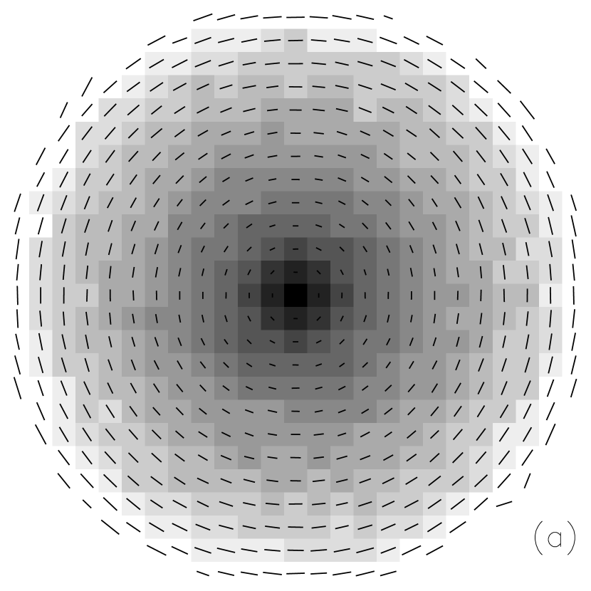
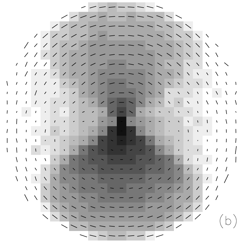
Figure 2: Example images of the DIRTY model are shown for a spherical system (a) and a conical system (b). The spherical system is an example of a reflection nebula with an embedded star. The conical system is an example of a bipolar nebula or a quasi-stellar object with an opening angle of 45$\arcdeg$ and an inclination of 30$\arcdeg$ with the bottom lobe tilted toward the observer. The grayscale displays the distribution of scattered light and the line segments the strength and orientation of the polarization. The maximum length of the line segments corresponds to a polarization of 48% (a) and 56% (b).

Figure 2 illustrates the images produced by the DIRTY model. Figure 2a shows how a spherical nebula with a central illuminating star would look in the V band assuming Milky Way type dust with a homogeneous distribution and a radial $\tau_{V}=1$. Figure 2b shows how a biconical nebula or active galactic nucleus inclined by an angle of 30$\arcdeg$ would look in the V band assuming Milky Way type dust with a homogeneous distribution and a $\tau_{V}=1$. Figure 3 displays the spectral energy distribution before and after the inclusion of dust in a simple starburst system. This is a good illustration of how the dust redistributes energy from the ultraviolet to the infrared. In addition, the three components (thermal equilibrium, thermal non-equilibrium, and aromatic feature emissions) of the dust emission spectrum are shown. Starburst systems are investigated in detail in Misselt et al. (2000a).

Figure 3: The spectral energy distribution (SED) of a starburst stellar population is plotted with and without dust. The stellar population is for constant star formation of 1.6 $M_{\sun}/year$ for a duration of 100 million years. The dust is Milky Way-like with a $\tau_{V}=1$. The dust distribution is the clumpy SHELL geometry (see Misselt et al. (2000a) for additional details).

3 Summary and Discussion

We have presented the DIRTY radiative transfer model in this paper and a companion paper (Misselt et al., 2000a). This model uses Monte Carlo techniques to compute the radiative transfer of photons emitted from arbitrary stellar distributions through arbitrary dust distributions. The weighting scheme used in the DIRTY model results in the efficient computation of the appearance of such systems from any viewing direction. The dust re-emission includes equilibrium thermal emission, non-equilibrium thermal emission, and the aromatic feature emission. The dust emission is computed self-consistently with the dust absorption and scattering using an iterative technique. The details of the dust emission are described by Misselt et al. (2000a).

The DIRTY model can be used to study a wide range of astrophysical objects due to its flexibility. The general behavior of multi-phase dust has been studied using the DIRTY model in reflection nebula environments (Witt & Gordon, 1996) and galactic environments (Witt & Gordon, 2000). The very non-symmetric reflection nebula surrounding the R CrB star UW Cen was successfully modeled using the DIRTY model (Clayton et al., 1999). The optical depth of spiral galaxies was investigated using an early version of the DIRTY model (Kuchinski et al., 1998). The finding that the lack of a 2175 Å depression in the spectra of UV-selected starburst galaxies was not due to radiative transfer effects but due to the dust grain properties was accomplished with the DIRTY model (Gordon et al., 1997). The ultraviolet through near-IR spectral energy distribution of the M33 nucleus was modeled using the DIRTY model and discovered to be a post-starburst stellar population surrounded by a shell of Milky Way-like dust (Gordon et al., 1999). The general behavior of the infrared emission of starburst galaxies has been studied by Misselt et al. (2000a). The full ultraviolet through far-infrared spectral energy distributions of a handful of starburst galaxies was studied by Misselt, Gordon, & Clayton (2000b). The range of objects which the DIRTY model has already been applied to is a good illustration of the usefulness of such a radiative transfer model.

In addition to continuing to use the DIRTY model to explore the nature of dust and its affects on a variety of astrophysical systems, we plan to continue to improve the model itself. One such improvement would be to modify the current way the dust distribution is stored to allow for grid points to be subdivided independently allowing for a larger range of size scale to be efficiently modeled (Wolf, Henning, & Stecklum, 1999). For example, this would allow for modeling the physically small region near the accretion disk in a QSO while simultaneously modeling the large scattering regions in the jets of the QSO. Another improvement would be to include electron scattering which would improve the application of the DIRTY model to the study of QSOs. Finally, the code could be parallelized to allow larger dust distribution grids to be studied in shorter amounts of time.

As there are always more interesting astrophysical systems to be studied than time in the day, anyone interested in using the DIRTY model should contact the authors for possible collaboration.

References

- Bianchi, Davies, & Alton (2000) Bianchi, S., Davies, J. I., & Alton, P. B. 2000, A&A, 359, 65
- Bianchi et al. (2000) Bianchi, S., Ferrara, A., Davies, J. I., & Alton, P. B. 2000, MNRAS, 311, 601
- Bianchi, Ferrara, & Giovanardi (1996) Bianchi, S., Ferrara, A., Giovanardi, C. 1996, ApJ, 465, 127
- Bohren & Huffman (1983) Bohren, C. F. & Huffman, D. R. 1983, Absorption and Scattering of Light by Small Particles (New York: Wiley)
- Calzetti et al. (1995) Calzetti, D., Bohlin, R. C., Gordon, K. D., Witt, A. N., Bianchi, L. 1995, ApJ, 446, L97
- Cashwell & Everett (1959) Cashwell, E. D. & Everett, C. J. 1959, A Practical Manual on the Monte Carlo Method for Random Walk Problems (New York: Pergamon)
- Clayton et al. (1999) Clayton, G. C., Kerber, F., Gordon, K. D., Lawson, W. A., Wolff, M. J., Pollacco, D. L., & Furlan, E. 1999, ApJ, 517, L143
- Clayton et al. (2000) Clayton, G. C., Wolff, M. J., Gordon, K. D., & Misselt, K. A. 2000, Thermal Emission Spectroscopy and Analysis of Dust, Disks, and Regoliths, ASP Conf. Ser. Vol. 196, eds. M. L. Sitko, A. L. Sprague, & D. K. Lynch (San Francisco: ASP), 41
- Code & Whitney (1995) Code, A. D. & Whitney, B. A. 1995, ApJ, 441, 400
- Colomb, Pöppel, & Heiles (1980) Colomb, F. R., Pöppel, W. G. L., & Heiles, C. 1980, A&AS, 40, 47
- Fischer, Henning, & Yorke (1994) Fischer, O., Henning, Th., & Yorke, H. W. 1994, A&A, 284, 187
- Gordon et al. (1997) Gordon, K. D., Calzetti, D., & Witt, A. N. 1997,ApJ, 487, 625
- Gordon et al. (2000) Gordon, K. D, Clayton, G. C., Witt, A. N., & Misselt, K. A. 2000, ApJ, 533, 236
- Gordon et al. (1999) Gordon, K. D., Hanson, M. M., Clayton, G. C., Rieke, G. H., & Misselt, K. A. 1999a, ApJ, 519, 165
- Gordon et al. (1994) Gordon, K. D., Witt, A. N., Carruthers, G. R., Christensen, S. A., & Dohne, B. C. 1994, ApJ, 432, 641
- Kim, Martin, & Hendry (1994) Kim, S.-H., Martin, P. G., Hendry, P. D. 1994, ApJ, 422, 164
- Kuchinski et al. (1998) Kuchinski, L. E., Terndrup, D. M., Gordon, K. D., & Witt, A. N. 1998, AJ, 115, 1438
- Manzini & di Serego Alighieri (1996) Manzini, A. & di Serego Alighieri, S. 1996, A&A, 311, 79
- Mishchenko, Hovenier, & Travis (2000) Mishchenko, M. I., Hovenier, J. W. & Travis, L. D. 2000, in Light Scattering by Nonspherical Particles: Theory, Measurements, and Applications (New York: Academic Press), 3
- Misselt, Gordon, & Clayton (2000b) Misselt, K. A., Gordon, K. D., & Clayton, G. C. 2000b, ApJ, in preparation
- Misselt et al. (2000a) Misselt, K. A., Gordon, K. D., Clayton, G. C., & Wolff, M. J. 2000a, ApJ, submitted
- Rosen & Bregman (1995) Rosen A. & Bregman, J. N. 1995, ApJ, 440, 634
- Scalo (1990) Scalo, J. 1990, in Physical Processes in Fragmentation & Star Formation, eds. R. Capuzzo-Dolcetta et al. (Dordrecht: Kluwer)
- Silva et al. (1998) Silva, L., Granato, G. L., Bressan, A., & Danese, L. 1998, ApJ, 509, 103
- Press, Teukolsky, Vetterling, & Flannery (1992) Press, W. H., Teukolsky, S. A., Vetterling, W. T., & Flannery, B. P. 1992, Numerical Recipes in C (Cambridge Univ. Press: Cambridge)
- Városi & Dwek (1999) Városi, F. & Dwek, E. 1999, ApJ, 523, 265
- Voshchinnikov & Karjukin (1994) Voshchinnikov, N. V. and Karjukin, V. V. 1994, A&A, 288, 883
- Whitney & Hartmann (1992) Whitney, B. A. & Hartmann, L. 1992, ApJ, 395, 529
- Witt (1977) Witt, A. N. 1977, ApJS, 35, 1
- Witt & Gordon (1996) Witt, A. N. & Gordon, K. D. 1996, ApJ, 463, 681
- Witt & Gordon (2000) Witt, A. N. & Gordon, K. D. 2000, ApJ, 528, 799
- Witt, Thronson, & Capuano (1992) Witt, A. N., Thronson, H. A., & Capuano, J. M. 1992, ApJ, 393, 611
- Witt et al. (1982) Witt, A. N., Walker, G. A. H., Bohlin, R. C., & Stecher, T. P. 1982, ApJ, 261, 492
- Wolf, Fischer, & Pfau (1998) Wolf, S., Fischer, O., Pfau, W. 1998, A&A, 340, 103
- Wolf, Henning, & Stecklum (1999) Wolf, S., Henning, Th., & Stecklum, B. 1999, A&A, 349, 839
- Wood et al. (1998) Wood, K., Kenyon, S. J., Whitney, B., & Trunbull, M. 1998, ApJ, 497, 404
- Wood & Jones (1997) Wood, K. & Jones, T. J. 1997, AJ, 114, 1405
- Wood & Reynolds (1999) Wood, K. & Reynolds, R. J. 1999, ApJ, 525, 799
- Young (2000) Young, S. 2000, MNRAS, 312, 567
- Yusef-Zadeh, Morris, & White (1984) Yusef-Zadeh, F., Morris, M., & White, R. L. 1984, ApJ, 278, 186
- Zubko & Laor (2000) Zubko, V. G. & Laor, A. 2000, ApJ, 128, 245