Chapter 1 Galaxies: from Kinematics to Dynamics

Michael R Merrifield
School of Physics & Astronomy, University of Nottingham, UK

1 Introduction

As will be apparent to anyone reading this book, the practitioners of N-body simulations have an enormous variety of preoccupations. Some are essentially pure mathematicians, who view the field as an exciting application for abstruse theory. Others enjoy formulating and tackling mathematically-neat problems, with little concern over whether the particular restrictions that they impose are also respected by nature. Still others are closer to computer scientists, inspired by the challenge of developing ever more sophisticated algorithms to tackle the N-body problem, but showing less interest in the ultimate application of their codes to solving astrophysical problems. This contribution is presented from yet another biased perspective: that of the observational galactic dynamicist. Observational astronomers tend to use N-body simulations in a rather cavalier manner, both as a tool for interpreting existing astronomical data, and as a powerful technique by which new observations can be motivated. The aim of this article is to illustrate this profitable interplay between simulations and observations in the study of galaxy dynamics, as well as highlighting a few of its shortcomings.

To this end, the text of this chapter is laid out as follows. Section 2 provides an introduction to the sorts of data that can be obtained in order to study the dynamical properties of galaxies, and goes on to discuss the intrinsic stellar dynamics that one is trying to model with these observations, and the role that N-body simulations can play in this modeling process. Section 3 gives a brief overview of the historical development of N-body simulations as a tool for studying galaxy dynamics. Section 4 provides some examples of the interplay between observations and N-body simulations in the study of elliptical galaxies, while Section 5 provides further examples from studies of disk galaxies, concentrating on barred systems. These sections are in no way intended to be encyclopedic in scope; rather, by selecting a few examples and examining them in some detail, the text seeks to give some flavour for the range of what is possible in this rich field. Finally, Section 6 contains some speculations as to what may lie in the future for this productive relationship between observations and N-body modeling.

2 Kinematics and Dynamics

The astronomer can glean only limited amounts of information about galaxies from observations. Some of these limitations arise from the practical shortcomings of telescopes, which can only obtain data with finite signal-to-noise ratios and limited spatial resolution. However, some of the restrictions are more fundamental – one can, for example, only view a galaxy from a single viewpoint, from which it is not generally possible to reconstruct its full three-dimensional shape, even if the galaxy is assumed to be axisymmetric (Rybicki 1986). We must therefore draw a distinction between kinematics, which are the observable properties relating to the motions of stars in a galaxy, and dynamics, which fully describe the intrinsic properties of a galaxy in terms of the motions of its component stars. Much of the study of galaxy dynamics involves attempting to interpret the former in terms of the latter.

Since stars are not the only constituents of galaxies, there is often additional information that one can glean from other components such as gas, whose kinematics may be revealed by its emission lines. These additional components can also confuse the issue, as selective obscuration by dust of some regions of a galaxy can have a major impact on the observed kinematics (e.g. Davies 1991). However, this text is concerned with N-body models, which are primarily used to describe the stellar components of galaxies, so here we concentrate just on the stellar dynamics. Nevertheless, it should be borne in mind that no description of a galaxy, particularly a later-type spiral system, is complete without considering these other components.

2.1 Kinematics

We begin by looking at what properties of a dynamical stellar system are, at least in principle, observable. The simplest data that one can obtain is what is detected by an image – the distribution of light from the galaxy on the sky, $\mu(x,y)$. Even for relatively nearby galaxies, the smallest resolvable spatial element will contain the light from many stars, so $\mu$ provides a measure of the number of stars per unit area on the sky.

Figure 1: Spectra of a star and a galaxy, showing how the absorption lines in the latter are shifted and broadened relative to the former.

By obtaining spectra of each of these spatial elements, we can start measuring the motions of the stars as well as their current locations. The observed spectrum will be a composite of the light from all the individual stars. Stellar spectra contain dark absorption lines due to the various elements in their atmospheres, but these absorption lines will be Doppler shifted by different amounts, depending on the line-of-sight velocities of the stars. Thus, as Figure 1 illustrates, the observed absorption lines will appear broadened and shifted due to the superposition of all the individual Doppler shifted spectra. Put mathematically, the observed spectrum of a galaxy made up from a large number of identical stars will be

$$G(u)=\int{\rm d}v_{\rm los}F(v_{\rm los})S(u-v_{\rm los}),$$ (1)

where $u=c\ln\lambda$ is the wavelength expressed in logarithmic units, $S$ is the spectrum of the star in the same units, and $F(v_{\rm los})$ is the function describing the distribution of stars’ line-of-sight velocities within the element observed.

Equation 1 is a convolution integral equation, which, in principle, can be inverted to yield the kinematic quantity of interest, $F(v_{\rm los})$, for a given galaxy spectrum, $G(u)$, and a spectrum $S(u)$ obtained using an observation of a suitable nearby “template” star. In practice, such unconstrained deconvolutions are hopelessly unstable. The usual approach is therefore to assume some relatively simple functional form for this function, and adjust its parameters until Equation 1 is most closely obeyed. The best-fitting version of $F(v_{\rm los})$ then provides a model for the line-of-sight velocity distribution of stars at that point. Conventionally, and with little physical justification, $F(v_{\rm los})$ has usually been assumed to be Gaussian, and the fitting returns optimal values for the mean velocity and dispersion of this model velocity distribution. More recently, however, the quality of data has improved to a point where more general functional forms can be fitted, allowing a less restricted analysis (e.g. Gerhard 1993, Kuijken & Merrifield 1993). With spectra at high signal-to-noise ratios, it is even possible to attempt a non-parametric analysis, yielding a best-fit form for $F(v_{\rm los})$ subject only to the most generic constraints of positivity and smoothness (e.g. Merritt 1997).

Although there are many practical difficulties involved in deriving a completely general description for $F(v_{\rm los})$ [see Binney & Merrifield (1998) Chapter 11], it is at least in principle measurable. Thus, the most general kinematic quantity that one can infer for a stellar dynamical system is the line-of-sight velocity distribution at each point on the sky where any of the galaxy’s stars are to be found, $F(x,y,v_{\rm los})$.

2.2 Dynamics

To fully specify a galaxy’s stellar dynamics, we need to know the gravitational potential, $\Phi(x,y,z)$, which dictates the motions of individual stars, and the “distribution function”, $f(x,y,z,v_{x},v_{y},v_{z})$, which specifies the phase density of stars, giving their velocity distribution and density at each point in the galaxy.

We would therefore appear to have a completely intractable problem, since we must somehow try to extract the six-dimensional distribution function from the rather complex observable projection of this quantity, $F(x,y,v_{\rm los})$, which only has three dimensions. Fortunately, however, the form of the distribution function is not completely arbitrary. For example, it must be positive or zero everywhere, since one can never have a negative density of stars. Further, stars are (more-or-less) conserved as they orbit around a galaxy, and can only change their velocities in a continuous manner, dictated by acceleration due to gravity. This continuity can be expressed in the collisionless Boltzmann equation,

$${{\rm d}f\over{\rm d}t}={\partial f\over\partial t}+{\bf v}\cdot\kern-0.24994pt\hbox{$\nabla$}\kern-8.33336pt\kern 0.50003pt\hbox{$\nabla$}\kern-8.33336pt\kern-0.24994pt\raise 0.43304pt\hbox{$\nabla$}f-\kern-0.24994pt\hbox{$\nabla$}\kern-8.33336pt\kern 0.50003pt\hbox{$\nabla$}\kern-8.33336pt\kern-0.24994pt\raise 0.43304pt\hbox{$\nabla$}\Phi\cdot{\partial f\over\partial{\bf v}}=0.$$ (2)

By manipulating the collisionless Boltzmann equation, one can derive a number of useful formulae for galaxy dynamics. A full discussion of this field is beyond the scope of this article, and the interested reader is referred to the excellent treatment by Binney & Tremaine (1987). Here, we simply summarize some of the key results:

• By taking a spatial moment of the collisionless Boltzmann equation, one can derive the virial theorem, which relates the total kinetic and potential energies of the system. The kinetic energy can be estimated from the observable line-of-sight motions of stars, from which the potential energy and hence the mass of the system can be inferred. It was this approach that provided the first evidence of dark matter, in clusters of galaxies (Zwicky 1937).

• By integrating Equation 2 over velocity, one obtains the continuity equation, which describes how the density of stars will vary with time due to any net flows in their motions. This equation is central to the dynamics of “cooler” stellar systems like disk galaxies, where mean streaming motions dominate the dynamics; as we shall see below, it has played an important role in studying the properties of barred galaxies.

• By multiplying Equation 2 by powers of velocity and integrating over velocity, one can derive the Jeans equations obeyed by the velocity dispersion, and their higher-moment analogues. The Jeans equations describe the random motions of stars, and have proved particularly important in studies of the dynamics of elliptical galaxies, where there is little mean streaming, and random velocities are generally the dominant stellar motions (e.g. Binney & Mamon 1982).

• By considering integrals of motion, one can derive the strong Jeans theorem: “for a steady state galaxy in which almost all the orbits are regular, the distribution function depends on at most three integrals of motion.” For example, in an axisymmetric galaxy, one may write $f(x,y,z,v_{x},v_{y},v_{z})\equiv f(E,J_{z},I_{3})$, where $E$ is the energy of the star, $J_{z}$ its angular momentum about the axis of symmetry, and $I_{3}$ is the “third integral” respected by the star’s orbit, which cannot generally be written in a simple analytic form.

This last result provides us with at least the hope that galaxy dynamics presents a tractable problem, since we now need only infer a three-dimensional distribution function from its three-dimensional observable projection, $F(x,y,v_{\rm los})$.

Equation 2 describes the continuity equation of a phase space fluid, which must be solved in order to understand the dynamics of galaxies. N-body simulation codes are really just Monte Carlo integrators tailored to solving this partial differential equation. It is very tempting to interpret the bodies in an N-body code as something more physical, such as the individual stars in a galaxy. However, unlike star clusters, galaxies contain so many stars that current simulations are still several orders of magnitude away from such a one-to-one correspondence. It is therefore much healthier to view an N-body simulation simply as a Monte Carlo solver for the collisionless Boltzmann equation, which is, in turn, a fluid approximation to the description of the properties of the large (but finite) collection of stars that make up a galaxy.

3 A Brief History of Galaxy N-body Simulations

Before launching into a discussion of modern applications of N-body simulations to studies of galaxy dynamics, it is instructive to look at the historical development of the field. N-body simulations of galaxies date back to well before the invention of the computer. Probably the first example of the technique was presented by Immanuel Kant in his 1755 publication, Universal Natural History and Theory of the Heavens. Part of this book was concerned with the properties of the Solar System, discussing how the plane of the ecliptic reflects the ordered motions of the planets around the Sun, while the more random orbits of comets causes them to be distributed in a spherical halo. Kant’s N-body simulation involved using this understanding of the Solar System as an analog computer by which the Milky Way could be simulated. He pointed out that the same law of gravity applies to the stars in the Galaxy as to the planets in the Solar System. He therefore argued that the band of the Milky Way could be understood in the same way as the plane of the ecliptic, arising from the ordered motion of the stars around the Galaxy. The lack of apparent motion in the stars could be explained by the vastly larger scale of the Milky Way. He further pointed out that the scattering of isolated stars and globular clusters far from the Galactic plane could be compared to comets, their locations reflecting their more random motions. Finally, he speculated that other faint fuzzy nebulae were similar “island universes” whose stars followed similar orbital patterns. Quite amazingly, Kant’s simple analog N-body simulation had revealed most of the key dynamical properties of galaxies.

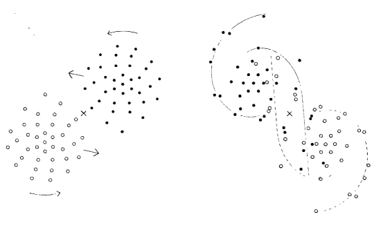
Figure 2: Holmberg’s original N-body simulation illustrating a merger between two disk galaxies. [Reproduced from Holmberg (1941).]

The next major advance in galaxy N-body simulations was made by Holmberg (1941). He used the fact that the intensity of a light source drops off with distance in the same inverse-square manner as the force of gravity. He therefore constructed an analogue computer by arranging 74 light bulbs on a table: the intensity of light arriving at the location of each bulb from different directions told him how large a force should be applied at that position, and hence how that particular bulb’s location should be updated. With this analogue integrator, Holmberg was able to show that collisions between disk galaxies can throw off tidally-induced spiral arms (see Figure 2), and that this process can rid the system of sufficient energy that the remaining stars can become bound into a single object.

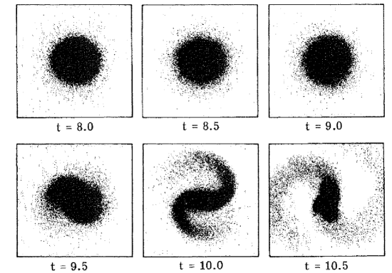
Figure 3: N-body simulation of a disk of “cold” particles initially orbiting on orbits very close to circular. Note the rapid growth of a strong bar instability. [Reproduced from Hohl (1971).]

The subject really took off in the 1970s with the widespread availability of digital computers of increasing power. Numerical N-body simulations on such a machine allowed Toomre & Toomre (1972) to explore the parameter space of galaxy mergers far more thoroughly than Holmberg had been able. They were thus able to reproduce the observed morphology of tidal tails and other features seen in particular merging galaxies, allowing them to reconstruct the physical parameters of the collisions in these systems. Other fundamental insights into galaxies were also made by N-body simulations around this time, such as the demonstration that a self-gravitating axisymmetric disk of stars on circular orbits is grossly unstable, rapidly evolving into a bar and spiral arms (see Figure 3).

More recently, progress has been driven by developments in algorithms and computer hardware, which allow N-body codes to follow the motions of ever larger numbers of particles. Although we are still a long way from being able to follow the motions of the billions of stars that make up a typical galaxy, the increased number of particles helps suppress various spurious phenomena that arise from the Poisson fluctuations in simulations using small numbers of particles. The increased number of particles also increases the dynamic range of scales that one can model within a single simulation. For example, it is now possible to look in some detail at the results of mergers between disk galaxies; it is has long been suggested that such mergers may produce elliptical galaxies [see Barnes & Hernquist (1992) for a review], but the simulations are now so good that we can measure quite subtle details of the merger remnants’ properties such as how fast they rotate and the exact shapes of their light distributions (Naab et al. 1999). We can then compare these quantities with the properties of real elliptical galaxies to test the viability of this formation mechanism. We are fast reaching the stage where a single simulation will have sufficient resolution to model simultaneously the growth of large-scale structure in the Universe and the formation of individual galaxies (e.g. Kay et al. 2000, Navarro & Steinmetz 2000). Thus, within the next few years, we will be able to perform simulations where the formation and evolution of galaxies can be viewed within the broader cosmological framework. However, since these studies depend critically on the treatment of gas hydrodynamics, they lie beyond the remit of this article on N-body analysis of the collisionless Boltzmann equation.

4 Modeling Elliptical Galaxies

Elliptical galaxies provide a good place to start in any attempt to model the stellar dynamics of galaxies. The simple elliptical shapes of these systems offers some hope that their dynamics may also be relatively straightforward to interpret; this high degree of symmetry means that the assumption of axisymmetry or even spherical symmetry may not be unreasonable. Further, the absence of dust in these systems means that the observed light accurately reflects the distribution of stars in the galaxy, greatly simplifying the modeling process.

In fact, elliptical galaxies are so simple that N-body simulations would not appear to have much of a role to play. The symmetry of these systems means that one can readily generate spherical or axisymmetric models with analytic distribution functions that reproduce many of the general properties of elliptical galaxies (e.g. King 1966, Wilson 1975). Where one seeks to reproduce the exact observations of a particular galaxy, Schwarzschild’s method (Schwarzschild 1979) is often a much better tool than a full N-body simulation. This technique involves adopting a particular form for the gravitational potential – perhaps, for example, by assuming that the mass distribution follows the light in the galaxy – and calculating a large library of possible stellar orbits in this potential. One then simply seeks the weighted superposition of these orbits that best reproduces all the observational data for the galaxy. Originally, these fits were made just to reproduce the projected distribution of stars, but more recent implementations have also used kinematic constraints such as the line-of-sight streaming velocities and velocity dispersions at different projected locations in the galaxy. It is also possible to start using information from the detailed shape of the line-of-sight velocity distribution (e.g. Cretton et al. 2000); ultimately, one could look for the superposition of orbits that reproduces the entire projected kinematics, $F(x,y,v_{\rm los})$.

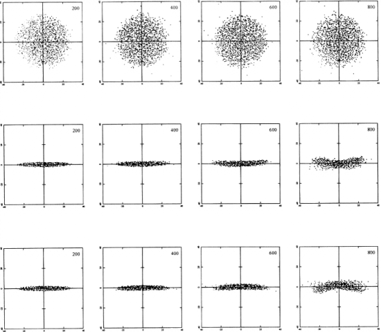
Figure 4: N-body simulation of an elliptical galaxy set up in an initially very flat distribution, as viewed along the three principal axes. Note the rapid fattening via a bending instability. [reproduced from Jessop et al. (1997).]

There are, however, some aspects of the properties of elliptical galaxies where N-body simulations offer a powerful tool. In particular, if one is concerned with the stability of an elliptical galaxy, one needs to study the full non-linear time evolution of Equation 2, for which N-body solutions are the most natural technique. As an example of the sort of issues one can answer using this approach, consider the distribution of elliptical galaxy shapes. Observations of this distribution have revealed that very flattened elliptical galaxies do not exist: the most squashed systems have shortest-to-longest ratios of only $\sim 0.3$. This observation could not be explained using the simple modeling techniques described above, since it is straightforward to derive a distribution function corresponding to a much flatter elliptical galaxy. However, if one takes such a distribution function as the initial solution to Equation 2, and uses an N-body simulation to follow its evolution, one discovers that it is grossly unstable, usually to some form of buckling mode, which rapidly causes it to evolve into a rounder system, comparable to the flattest observed ellipticals (see Figure 4). Thus, the absence of flatter elliptical systems has a simple physical explanation: they are dynamically unstable.

Instability analysis using N-body codes has also shed light on other properties of elliptical galaxies. For example, Newton & Binney (1984) successfully constructed a distribution function that could reproduce the photometric and kinematic properties of M87: assuming only that the mass of the galaxy were distributed in the same way as its light and that the galaxy is spherical, they were able to match both the light distribution of M87 and the variation in its line-of-sight velocity dispersion with projected radius. Thus, they would appear to have a completely viable dynamical model for M87. However, Merritt (1987) took this distribution function as the starting point for an N-body simulation, and showed that the preponderance of stars on radial orbits at its centre rendered the model unstable – the N-body model rapidly formed a bar at its centre. Thus, the simple spherical model in which the mass followed the light was invalidated, implying either that M87 is not intrinsically spherical, or that it contains mass in addition to that contributed by the stars.

Although some instability analyses can be carried out analytically, the full calculations of the behaviour of an unstable system, particularly once the instability has grown beyond the linear regime, is almost always intractable, making N-body simulations the best available tool. Some care must be taken, however, to make sure that any instability detected is not a spurious effect arising from the numerical noise in the Monte Carlo N-body integration method (or indeed, that any real instability is not suppressed by the limitations of the method).

N-body simulations can also be applied to the study of elliptical galaxies by providing what might be termed “pseudo-data.” When a new technique is proposed for extracting the intrinsic dynamical properties of a galaxy from its observable kinematics, one needs some way of testing the method. Ideally, one would take a galaxy with known dynamical properties, and see whether the method is able to reconstruct those properties. Unfortunately, it is most unlikely that the corresponding intrinsic dynamics of a real galaxy would be known – if they were, there would be no need to develop the new technique! However, with an N-body simulation, for which the intrinsic properties are all measurable, one can readily calculate the appropriate projections to construct its “observable” properties, $F(x,y,v_{\rm los})$, from any direction. One can then test the method on these pseudo-data to see whether the intrinsic properties of the galaxy can be inferred.

An excellent example of this approach was provided by Statler (1994) in his attempt to reconstruct the full three-dimensional shapes of elliptical galaxies from their observable kinematics. Although these systems have a simple apparent structure, there is no a priori reason to assume that they are axisymmetric, and a more general model would be to suppose that they are triaxial, with three different principal axis lengths (like a somewhat deflated rugby ball). Indeed, there is strong observational evidence that elliptical galaxies cannot all be completely axisymmetric. Images of some ellipticals reveal that the position angles on the sky of their major axes vary with radius. Such “isophote twist” cannot occur if a galaxy is intrinsically axisymmetric, as the observed principal axes of such a system would always coincide with the projection on the sky of its axis of symmetry. Thus, these elliptical galaxies must be triaxial in structure. Statler made a study of the dynamics of some simple triaxial galaxy models, and concluded that one could obtain a much better measure of the shape of the system by considering the mean line-of-sight motions of stars as well as their spatial distribution. As a test of this hypothesis, he took an N-body model, and extracted from it the observable properties of the mean line-of-sight velocity and projected density at a number of positions. Unfortunately, the constraints on the intrinsic galaxy shape inferred from these data were found to be only marginally consistent with the true known shape of the N-body model. Although in some ways rather disappointing, this analysis reveals the true power of using N-body simulations to test such ideas: the N-body simulation did not contain the same simplifying assumptions as the analytic model that had originally motivated the proposed idea, so it provided a truly rigorous test of the technique.

As a final example of the way in which N-body simulations can interact with observations in the study of elliptical galaxies, let us turn to some work on “shell galaxies.” Such systems typically appear to be fairly normal ellipticals, but careful processing of deep images reveals that their light distributions also contain faint ripple-like features in a series of arcs around the galaxies’ centres (e.g. Malin & Carter 1983). The simplest explanation for these shells is that they are the remains of a small galaxy that is merging with the larger elliptical from an almost radial orbit. Each shell is made up from stars of equal energy from the infalling galaxy, which have completed a half-integer set of oscillations back-and-forth through the larger galaxy, and are in the process of turning around. Since the stars slow to a halt as they turn around, they pile up at these locations, producing the observed shells. Shells at different radii contain stars with different energies, which have completed different numbers of radial orbits since the merger. Since the stars in any shell have a very small velocity dispersion compared to that of the host galaxy, they show up clearly as sharp edges in the photometry.

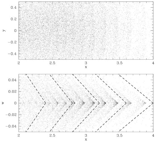
Figure 5: N-body simulation, projected to show the observable properties of the shells created in a minor merger. The upper panel shows the photometric properties, while the lower panel shows the kinematically-observable line-of-sight velocity versus projected distance along the major axis. The dashed lines show the predicted caustic shapes. [Reproduced from Kuijken & Merrifield (1998)].

N-bodies simulations (e.g. Quinn 1984) played a key role in confirming that such mergers could, indeed, produce sets of faint shells in the photometric properties of galaxies. It is therefore interesting to go on to ask what the most generally-observable kinematic properties of one of these shells might be. Again, N-body simulation offer an excellent tool with which to address this question. Figure 5 presents the results of such a simulation, showing both the faint photometric shells and the rather stronger kinematic signature of a minor merger. The line-of-sight velocity distribution as a function of position along the major axis shows a characteristic chevron pattern, whose origins are relatively straightforward to explain (Kuijken & Merrifield 1998). Consider the stars in a shell whose outer edge lies at $r=r_{s}$. By energy conservation, the radial velocities of stars at $r<r_{s}$ in this shell are

$$v_{r}=\pm\left\{2[\Phi(r_{s})-\Phi(r)]\right\}^{1/2},$$ (3)

where $\Phi(r)$ is the gravitational potential at radius $r$. By simple geometry, the observable line-of-sight component of this velocity is given by

$$v_{\rm los}^{2}=\left({z\over r}v_{r}\right)^{2}=2\left(1-{x^{2}\over r^{2}}\right)[\Phi(r_{s})-\Phi(r)].$$ (4)

Close to the shell edge, where $r\sim r_{s}\ll x$, the maximum value of $v_{\rm los}$ can be shown, by expanding and differentiating Equation 4, to be

$$v_{\rm max}=\pm\left({1\over r}{{\rm d}\Phi\over{\rm d}r}\right)^{1/2}(r_{s}-x).$$ (5)

Examples of lines obeying this equation are shown in Figure 5; they clearly match the pattern seen in the N-body “observation.” Thus, if one were to make a detailed kinematic observation of a shell galaxy and observed this chevron pattern, not only would one have dynamical evidence for the merger model, but one would also be able to use the slope of the chevrons to measure ${{\rm d}\Phi\over{\rm d}r}$ at the radii of each of the shells. Combining these measurements would allow one to estimate the gravitational potential of the galaxy in a simple robust manner.

Here, then, is an excellent example of the close interplay that is possible between observations and N-body simulations. The photometric discovery of shells in elliptical galaxies led to a merger theory that was validated by N-body simulations. N-body simulations then provided the motivation for further observations to study the kinematics of shells in order to make a novel measurement of the gravitational potentials of elliptical galaxies.

5 Modeling Disk Galaxies

We now turn to the use of N-body simulations in the study of disk galaxies. Here, the motivation for using N-body modeling is much clearer. Spiral galaxies contain a wealth of structure, much of which is probably transient in nature, so simple analytic models of the type that do such a good job of describing the basic properties of elliptical galaxies are clearly inappropriate. Instead, one needs a full time-dependent solution to Equation 2, for which N-body simulations provide the most obvious technique.

It should, however, be borne in mind that the use of Equation 2 is often significantly less appropriate in the study of disk galaxies than was the case for ellipticals. Active star formation in many spiral galaxies means that the continuity implied by the collisionless Boltzmann equation is not strictly valid, as stars appear in the formation process, and the brightest, most massive amongst them subsequently disappear in supernovae. Further, the location of these star formation regions is largely driven by the dynamics of the gas from which the stars form. The collisional nature of this gas means that it is poorly described by a collisionless N-body code, and should really be dealt with using much more sophisticated gas codes. As a further complication, the dust found in most spiral galaxies means that a significant fraction of the starlight is scattered or absorbed. Thus, there is a rather complicated relationship between the results of an N-body code (which essentially gives the distribution of stars in the system) and the observed photometric properties of a galaxy. Finally, the likely transient nature of many of the properties of spiral galaxies also complicates comparison between observation and theory: since one has only a snapshot view of a galaxy, one has to search through the complete evolution in time of an N-body simulation to see if it matches the observed properties of the galaxy at any point.

Despite these caveats, N-body simulations have provided a wide variety of insights into the dynamics of disk galaxies. As for the ellipticals, N-body simulations have not only been used to explain many of the observed properties of disk galaxies, but they have also provided data sets that can test novel analysis techniques, and they have provided the key motivation for a range of new observations.

As an example of this synergy between N-body simulations and observations, we consider in some detail the properties of barred galaxies. As we have already described in Section 3, one of the early triumphs of N-body simulations was in demonstrating that a rectangular bar-like structure, similar to those seen in more than a third of disk galaxies, appears due to an instability in a self-gravitating disk of stars. Subsequently, as we shall see below, N-body simulations have enabled us to understand a great deal about the properties of bars.

One of the simplest physical properties of a bar is its pattern speed, $\Omega_{p}$, which is the angular rate at which the bar structure rotates. In a simulation like that shown in Figure 3, $\Omega_{p}$ is easy enough to calculate by comparing the bar position angles at different times. In a real galaxy, of course, we do not have the luxury of being able to wait the millions of years required to see the bar pattern move, so it is less obvious that $\Omega_{p}$ can be measured. However, Tremaine & Weinberg (1984) elegantly demonstrated that one can manipulate the continuity equation into a form that contains only the distribution of stars, their mean line-of-sight velocities (observable via the Doppler shift in the starlight at each point in the galaxy), and $\Omega_{p}$. Since the pattern speed is the only unknown, one can derive its value directly from the other observable properties. At the time that this technique was proposed, no observations of barred galaxies had ever produced the quality of spectral data required to implement the method. However, Tremaine & Weinberg were able to prove its viability by taking a single snapshot of an N-body simulation and creating pseudo-observations of the line-of-sight velocities and projected locations of the objects in it. The pattern speed derived from this single pseudo-dataset was found to match that derived from watching the pattern rotate in the complete time sequence of the simulation.

More recently, kinematic observations have progressed to a point where this method can be applied to data from real barred galaxies (e.g. Merrifield & Kuijken 1995). These measurements led to the discovery that bar patterns seem to rotate rather rapidly, with the bar ends lying close to the “co-rotation radius,” which is the radius in the galaxy at which the bar pattern rotates at the same speed that the stars themselves circulate. This finding proved interesting in the light of subsequent N-body simulations of bars (Debattista & Sellwood 2000). These simulations showed that although bars form with this rapid initial rotation rate, in many cases the bar pattern speed rapidly decreases almost to a halt. This deceleration is the result of dynamical friction: the passage of the bar disturbs the orbits of any material orbiting in the halo of the galaxy, concentrating this material into “wakes” of mass that lie behind the rotating bar, exerting a torque that serves to slow the bar’s rotation. Since cosmological N-body models of galaxy formation predict that galaxies should form in centrally-concentrated dark matter halos with plenty of mass at small radii (e.g. Navarro, Frenk & White 1997), one would expect the dynamical friction effects from this halo mass to be strong, yielding slowly-rotating bars. Thus, either the bars with measured pattern speeds happen to have been caught very early in their lives when they have not slowed significantly, or the dark halos in which these barred galaxies reside do not conform to the cosmologists’ predictions.

Finally in this discussion of N-body studies of barred galaxies, let us turn to the ultimate demise of bars. Once a bar has grown, there are several ways that it can be destroyed. A minor merger with an in-falling satellite galaxy can put enough random motion into the stars to mean that they no longer follow highly-ordered bar-unstable orbits, thus destroying the bar [see, for example, the N-body simulations by Athanassoula (1996)]. A less violent solution involves the growth of a massive central black hole in the galaxy. Inside a bar, stars shuttle back and forth on ordered orbits aligned with the bar. However, N-body simulations have shown that if a central black hole exceeds a critical mass of a few percent of the bar mass, then the black hole scatters the passing stars so strongly that they end up on chaotic orbits that do not align with the bar, thus destroying its coherent shape (Sellwood & Moore 1999). This mechanism is particularly intriguing, as a bar provides a conduit by which material can be channeled toward the centre of a galaxy. If this inflowing matter is accreted by a central black hole, the central object’s mass can grow to a point where the bar is disrupted, shutting off any further inflow of material – a remarkable case of the black hole biting the hand that feeds it!

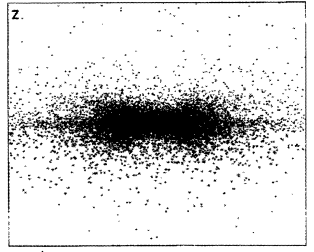
Figure 6: N-body simulation showing the peanut-shaped structure perpendicular to the disk plane into which a bar ultimately evolves. [Reproduced from Combes & Sanders (1981)].

Even if left in isolation with no mergers or central black holes, thin bars in disks can have only a very limited lifetime. N-body simulations (Combes & Sanders 1981, Raha et al. 1991) have shown that bars undergo a buckling instability perpendicular to the plane of the galaxy, rather similar to that shown in Figure 4. This instability initially just bends the bar, but the structure then flops back and forth until it fills a double-lobed fattened region perpendicular to the galaxy plane, rather like a peanut still in its shell (see Figure 6).

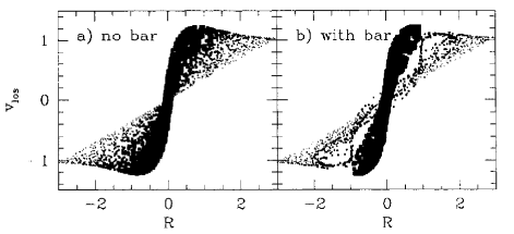
Figure 7: Simulations of the observable kinematics (line-of-sight velocity versus projected radius) along the major axes of edge-on galaxies, comparing the properties of barred and unbarred systems. [Reproduced from Kuijken & Merrifield (1995)].

This N-body discovery has an interesting tie-in with observations: the bulges of approximately a third of edge-on galaxies are observed to have boxy or peanut-shaped isophotes, similar to that seen in Figure 6 (de Souza & dos Anjos 1987). Could it be that these systems are simply barred galaxies viewed edge-on? The fraction certainly corresponds to the percentage of more face-on systems seen to contain bars, but some more direct evidence is clearly needed. Again, numerical simulations pointed the way forward: calculations of orbits in barred potentials have shown that they display a rich array of structure, with highly elongated orbits, and changes in orientation at radii where one passes through resonances. Kuijken & Merrifield (1995) investigated the implications of this complexity for the observable kinematics of edge-on barred galaxies, and showed that the structure is apparent even in projection: as Figure 7 shows, the changing orientations of the different orbit families shows up in a rather complex structure in the observable kinematics, $F(x,v_{\rm los})$. More sophisticated N-body and hydrodynamic simulations, allowing for the complex collisional behaviour of gas, confirm that this structure should also be apparent in the gas kinematics of an edge-on barred galaxy (Athanassoula & Bureau 1999).

This N-body analysis motivated detailed kinematic observations of edge-on disk galaxies, which revealed a remarkably strong correlation: systems in which the central bulge appears round almost all have the simple kinematics one would expect for an axisymmetric galaxy, whereas galaxies with peanut-shaped central bulges almost all display the complex kinematics characteristic of orbits in a barred potential (Bureau & Freeman 1999, Merrifield & Kuijken 1999). Thus, the connection between peanut shaped structures and bars suggested by the instability found in the N-body models has now been established in real disk galaxies. Here, then, is another excellent example of a case where N-body simulations have not only produced a prediction as to how galaxies may have evolved to their current structure, but have also provided the motivation for new kinematic observations that confirm this prediction.

6 The Future

Hopefully, the examples described in this article have given some sense of the productive interplay between kinematic observations of galaxies and N-body simulations of these systems, and there is every reason to believe that this relationship will continue to thrive as the fields develop. On the observational side, kinematic data sets become ever more expansive: the construction of integral field units for spectrographs has made it possible to obtain spectra for complete two-dimensional patches on the sky, thus allowing one to map out the complete observable kinematics of a galaxy, $F(x,y,v_{\rm los})$, in a single observation. In the N-body work, developments in computing power result in ever-larger numbers of particles in the code, allowing finer structure to be resolved, and giving some confidence that the results are not compromised by the limitations in the Monte Carlo solution of Equation 2. More powerful computers also allow one to analyze the completed N-body simulations more thoroughly: for example, when comparing transient spiral features in real galaxies to those in a simulation, one can search through the entire evolution of the simulation to see whether there are any times at which the data match the model.

Traditionally, one weakness in combining N-body analysis with kinematic observations is that although the simulations are very good at analyzing the generic properties of galaxies, they do not provide a useful tool for modeling the specific properties of individual objects. However, there is now the intriguing possibility that this shortcoming could be overcome, through Syer & Tremaine’s (1996) introduction of the idea of a “made-to-measure” N-body simulation. In such N-body simulations, in addition to its phase-space coordinates, each particle also has a weight associated with it. This weight can be equated with that particle’s contribution to the total “luminosity” of the model. Syer & Tremaine presented an algorithm by which the weights can be adjusted as the N-body simulation progresses, such that the observable properties of the model evolve in any way one might wish while still providing a good approximation to a solution to the collisionless Boltzmann equation. Thus, for example, one can take as a set of initial conditions a simple analytic distribution function, and “morph” this model into a close representation of a real galaxy. In fact, one can go beyond just the photometric properties of the galaxy, and match the N-body model to kinematic data as well, thus yielding a powerful dynamical modeling tool. Syer & Tremaine’s initial implementation of this method was fairly rudimentary: for example, they did not solve self-consistently for the galaxy’s gravitational potential, but instead imposed a fixed mass distribution. However, there appears to be no fundamental reason why a more complete made-to-measure N-body code could not be developed as a sophisticated technique for modeling real galaxy dynamics.

There has also been a lot of progress in the techniques of stellar population synthesis (e.g., Bruzual & Charlot 1993, Worthey 1994). This approach involves determining the combination of stellar types, ages and metallicities that could be responsible for integrated light properties of a galaxy such as its colours and spectral line strengths. Thus, one can now go beyond the simple-minded dynamicist’s picture of a galaxy made up from a large population of identical stars, as assumed in Section 2; instead, one can begin to pick out the range of ages and metallicities that could be present in a galaxy, and even ask whether the different populations have different kinematics. Here, an extension the made-to-measure N-body approach presents an exciting possibility. In addition to a weight, one could associate an age and a metallicity with each particle. One could then synthesize the stellar population associated with that particle, and hence calculate its contribution to the total spectrum of the galaxy. Projecting such an N-body model on to the sky, one could calculate the spectrum associated with any region of the model galaxy by simply adding up the spectral contributions from the individual particles (suitably Doppler shifted by their line-of-sight velocities). By using the sorts of N-body morphing techniques introduced by Syer & Tremaine (1996), one could then evolve an N-body simulation until it matched the properties of a real galaxy not only in its light distribution and kinematics, but also in its colours, the strengths of all its spectral absorption lines, etc. This complete spectral modeling – in essence, a galaxy model that would fit the spatial coordinates and energy of every detected photon – would represent the ultimate match between N-body simulations and observations. It would be a truly amazing tool for use in the study of galaxy dynamics, and would allow us to integrate the evolution of the galaxy’s stellar population into the dynamical picture, opening up a whole new dimension of information in the study of galaxy formation, evolution and structure.

References

Athanassoula, E. & Bureau, M., 1999, ApJ, 522, 699

Athanassoula, E., 1996, in Buta R., Croker D.A. and Elmegreen B.G., eds., Barred Galaxies, Astronomical Society of the Pacific, p. 307

Barnes, J.E. & Hernquist, L., 1992, ARA&A, 30, 705

Binney, J. & Mamon, G.A., 1982, MNRAS, 200, 361

Binney, J. & Merrifield, M., 1998, Galactic Astronomy, princeton University Press

Bruzual, A.G. & Charlot, S., 1993, ApJ, 405, 538

Bureau, M. & Freeman, K.C., 1999, AJ, 118, 126

Combes, F. & Sanders, R.H., 1981, A&A, 96, 164

Cretton, N., Rix, H.-W. & de Zeeuw, P.T., 2000, ApJ, 536, 319

Davies, J., 1991, in Sundelius B., ed, Dynamics of Disc Galaxies, Göteborg, p. 65

Debattista, V.P. & Sellwood, J.A., 2000, ApJ, 543, 704

de Souza, r.E. & dos Anjos, S., 1987, A&A, 70, 465

Gerhard, O.E., 1993, MNRAS, 265, 213

Hohl, F., 1971, ApJ, 168, 343

Holmberg, E., 1941, ApJ, 94, 385

Jessop, C.M., Duncan, M.J. & Levison, H.F., 1997, ApJ, 489, 49

Kay, S.T., et al., 2000, MNRAS, 316, 374

King, I., 1966, AJ, 71, 64

Kuijken, K. & Merrifield, M.R., 1993, MNRAS, 264, 712

Kuijken, K. & Merrifield, M.R., 1995, ApJ, 443, L13

Kuijken, K. & Merrifield, M.R., 1998, MNRAS, 297, 1292

Malin, D.F. & Carter, D., ApJ, 274, 534

Merrifield, M.R. & Kuijken, K., 1995, MNRAS, 274, 933

Merrifield, M.R. & Kuijken, K., 1999, A&A, 345, L47

Merritt, D., 1987, ApJ, 319, 55

Merritt, D., 1997, AJ, 114, 228

Naab, T., Burkert, A. & Hernquist, L., 1999, ApJ, 523, L133

Navarro, J.F., Frenk, C. & White, S.D.M., 1997, ApJ, 490, 493

Navarro, J.F. & Steinmetz, M., 2000, ApJ, 538, 477

Newton, A.J. & Binney, J., 1984, MNRAS, 210, 711

Quinn, P.J., 1984, ApJ, 279, 596

Raha, N., Sellwood, J.A., James, R.A. & Kahn, F.D., 1991, Nature, 352, 411

Rybicki, G.B., 1986, in de Zeeuw P.T., ed, Proc IAU Symp 127, The Structure and Dynamics of Elliptical Galaxies, Dordrecht, p. 397

Schwarzschild, M., 1979, ApJ, 232, 236

Sellwood, J.A. & Moore, E.M., 1999, ApJ, 510, 125

Statler, T., 1994, ApJ, 425, 500

Syer, D. & Tremaine, S., 1996, MNRAS, 282, 223

Toomre, A. & Toomre, J., 1972, ApJ, 178, 623

Wilson, C.P., 1975, AJ, 80, 175

Worthey, G., 1994, ApJS, 95, 107

Zwicky, F., 1937, ApJ, 86, 217