Inhomogeneous Big Bang Nucleosynthesis and the High Baryon Density Suggested by Boomerang and MAXIMA

Abstract

The recent Boomerang and MAXIMA data on the cosmic microwave background suggest a large value for the baryonic matter density of the universe, $\omega_{b}\sim 0.03$. This density is larger than allowed by standard big bang nucleosynthesis theory and observations on the abundances of the light elements. We explore here the possibility of accommodating this high density in inhomogeneous big bang nucleosynthesis (IBBN). It turns out that in IBBN the observed ${\rm D}$ and $Y_{p}$ values are quite consistent with this high density. However, IBBN is not able to reduce the ${}^{7}{\rm Li}$ yield by more than about a factor of two. For IBBN to be the solution, one has to accept that the ${}^{7}{\rm Li}$ plateau in population II halo stars is depleted from the primordial abundance by at least a factor of two.

I Introduction

The most accurate way to estimate the average density of baryonic matter in the universe, $\rho_{b}$, has for a long time been big bang nucleosynthesis. In standard big bang nucleosynthesis (SBBN)[3] the calculated primordial yields of the light elements depend only on the baryon-to-photon ratio $\eta\equiv n_{b}/n_{\gamma}$. Future precision measurements of the fluctuations in the cosmic microwave background (CMB) will provide another way of measuring the baryon density. The shape of the angular power spectrum of these fluctuations will depend on a number of cosmological parameters, among which is the baryon-to-photon ratio. In this context it is usually given as the baryonic contribution to the critical density times the Hubble constant squared, $\omega_{b}\equiv\Omega_{b}h^{2}$.

These two measurements rely on completely different physics, and if they agree it is an important confirmation that we have the right understanding of the early universe. Assuming that there was no significant entropy production[4] in the universe between BBN and recombination, the two parameters $\omega_{b}$ and $\eta$ are related via the present temperature of the CMB, $T=2.725$ K, by

$$\eta_{10}=274\omega_{b}.$$ (1)

Two recent balloon-borne experiments, Boomerang[5] and Maxima-1[6], have now provided us with the first measurements of the CMB angular power spectrum which are of sufficient quality that an estimate of $\omega_{b}$ can be made from them. The result[7], $\omega_{b}\sim 0.030$, is significantly higher than the SBBN result. Indeed, SBBN clearly cannot accommodate as high a baryon density as $\omega_{b}=0.030$[8].

The SBBN yields for $\omega_{b}=0.030$ are $Y_{p}=0.251$, ${\rm D}/{\rm H}=1.7\times 10^{-5}$, ${}^{3}{\rm He}/{\rm H}=8.4\times 10^{-6}$, and ${}^{7}{\rm Li}/{\rm H}=7.6\times 10^{-10}$. With the exception of ${}^{7}{\rm Li}$, the uncertainty in these SBBN yields is much less than the uncertainty in the primordial abundances derived from observations.

There is much debate about chemical evolution and systematic effects in observations. For the primordial helium abundance there are two competing estimates, the “low ${}^{4}{\rm He}$”[9], $Y_{p}=0.234\pm 0.003$ and the “high ${}^{4}{\rm He}$”[10], $Y_{p}=0.244\pm 0.002$. The difference is largely due to the method of estimating the present abundances from the observed line intensities, suggesting that the systematic uncertainty may be larger than the $\pm 0.005$ usually assumed[11].

Burles and Tytler [12] claim to have established the primordial deuterium abundance as ${\rm D}/{\rm H}=(3.3\pm 0.25)\times 10^{-5}$ (“low D”) based on Lyman-series absorption by high-redshift clouds. This is based on a detected low deuterium abundance in three such systems and upper limits from others. There remains one such system, where a high deuterium abundance, ${\rm D}/{\rm H}\sim 2\times 10^{-4}$ (“high D”), has been observed[13]. It may be that the accuracy of such observations has been overestimated[14]. We refer the reader to recent reviews[15] for further discussion and adopt the observational constraints $Y_{p}=0.228$–$0.248$, ${\rm D}/{\rm H}=2.9$–$4.0\times 10^{-5}$[16]. These lead to the SBBN range $\omega_{b}=0.004$–$0.021$ from $Y_{p}$ and $\omega_{b}=0.018$–$0.022$ from ${\rm D}/{\rm H}$. The “low D” of Burles and Tytler gives $\omega_{b}=0.020\pm 0.01$.

The “Spite plateau”[17] of ${}^{7}{\rm Li}$ abundance in population II halo stars provides us with the best estimate of the primordial lithium abundance. Bonifacio and Molaro[18] obtain a present lithium abundance $\log_{10}({}^{7}{\rm Li}/{\rm H})=-9.80\pm 0.012\pm 0.05$ for these stars, and argue against any significant depletion from the primordial abundance, based on the lack of dispersion in the data. Pinsonneault et al.[19] estimate a depletion factor of 0.2–0.4 dex from rotationally induced mixing. In a more recent study Ryan et al.[20] obtain a mean abundance $\log_{10}({}^{7}{\rm Li}/{\rm H})=-9.88$ for the Spite plateau, and argue that the narrow spread, less than 0.02 dex, limits depletion by rotationally induced mixing to less than 0.1 dex. Moreover, they observe a slight trend with metallicity, suggesting a galactic contribution, so that the primordial abundance could be lower than the observed abundance. Based on this, Ryan et al.[21] derive the range $\log_{10}({}^{7}{\rm Li}/{\rm H})=-10.04$…$-9.72$ for the primordial abundance. This very tight upper limit to primordial lithium is in conflict with the “low D” estimate[12], $\omega_{b}=0.020$, which corresponds to $\log_{10}({}^{7}{\rm Li}/{\rm H})=-9.5$ in SBBN.

At present there seems to be a consensus[19, 22, 23], that the primordial abundance cannot be larger than the observed value by more than about 0.4 dex, so that models producing a primordial lithium abundance above $\log_{10}({}^{7}{\rm Li}/{\rm H})=-9.4$, or ${}^{7}{\rm Li}/{\rm H}=4\times 10^{-10}$, would be ruled out. This gives an upper limit $\omega_{b}\leq 0.022$ in SBBN.

While the upper limit to $\omega_{b}$ from $Y_{p}$ is rather soft, the deuterium and lithium abundances are in clear conflict with $\omega_{b}=0.03$.

This CMB measurement of $\omega_{b}$ is rather preliminary and not very accurate, and thus it would be premature to discard the SBBN estimate. Since the CMB measurement is a simultaneous fit of many cosmological parameters, the lack of prominence of the second peak in the power spectrum could have another explanation. Suggestions include a significant tilt[24], an isocurvature component[25], or a feature[26] in the primordial perturbation spectrum, and topological defects[27].

Future satellite experiments, MAP[28] and Planck[29], will give us a better CMB determination of $\omega_{b}$. If the situation persists and the CMB value of $\omega_{b}$ turns out to be $\omega_{b}\sim 0.03$ or higher, one has to consider abandoning SBBN in favor of non-standard BBN[30]. There are many modifications suggested to standard BBN, some of which can accommodate a higher baryon density[31].

We consider here one such possible modification, inhomogeneous big bang nucleosynthesis (IBBN). In IBBN one assumes that the baryon density was inhomogeneous during BBN. This inhomogeneity could be an initial condition resulting from unknown physics in the early universe, or it could be the result of some physical event, like a phase transition, occurring before BBN.

The nature of IBBN depends on the distance scale of the inhomogeneity. Especially interesting is the case, where this distance scale is of the order of the neutron diffusion length during BBN[32]. Then neutron diffusion will lead to an inhomogeneity in the neutron-to-proton ratio. If the density contrast between high- and low-density regions is large enough, this ratio can exceed unity in the low-density region. In this case IBBN leads to a decrease in the ${}^{4}{\rm He}$ yield and an increase in the ${\rm D}$ yield, favoring larger $\omega_{b}$. However, the ${}^{7}{\rm Li}$ yield is more likely to increase than decrease from the SBBN result for the same average $\omega_{b}$.

In this paper we focus on the question, whether the high value $\omega_{b}=0.030$, corresponding to $\eta_{10}=8.22$, would be acceptable in IBBN. There have been many papers on IBBN[32]. However, because of the large number of parameters in the IBBN model, the parameter space has not been covered thoroughly in them. Focusing on one particular value of $\eta_{10}$ we reduce the dimension of the parameter space, allowing us to search the space of the remaining parameters more completely. We can thus give a more specific answer to the above question.

II Results

We have updated our IBBN code[33] with the latest compilation of reaction rates[34]. The new reaction rates have little impact on the isotope yields. The largest effect is on ${}^{7}{\rm Li}$ production, which is reduced by 5%. Vangioni-Flam et al.[35] estimate the uncertainty in ${}^{7}{\rm Li}$ yield due to reaction rates to be 30%. The actual uncertainty may be even larger, since their method of error estimation allows error compensation.

We assume a simple initial density profile, so that there is a high density region, with one baryon density ($\eta_{\rm high}$), and a low-density region with another baryon density ($\eta_{\rm low}$). Diffusion will then smooth out this initial density profile. We assume a spherically symmetric geometry, allowing us to study two different geometric configurations: 1) centrally condensed (CC), where we have a spherical high density region surrounded by a low density region, and 2) spherical shell (SS), where we have a spherical shell of high baryon density inside which we have low baryon density. The first case approximates a situation where the high density regions have a rather compact shape, with a low surface-to-volume ratio, the second case a situation where the high density regions have a more planar geometry, with a large surface-to-volume ratio.

Once the average baryon density $\eta$ is fixed, we have three remaining parameters, the density contrast $R\equiv\eta_{\rm high}/\eta_{\rm low}$, the volume fraction $f_{v}$ of the high-density region, and the distance scale $r$. There is an “optimum value” $r_{\rm opt}$ of the distance scale, related to the neutron diffusion scale, where the effect of the neutron excess is maximized. For very high density contrasts, $f_{v}R\gtrsim 100$ the results become independent of $R$. For a more detailed discussion, see Ref. [33].

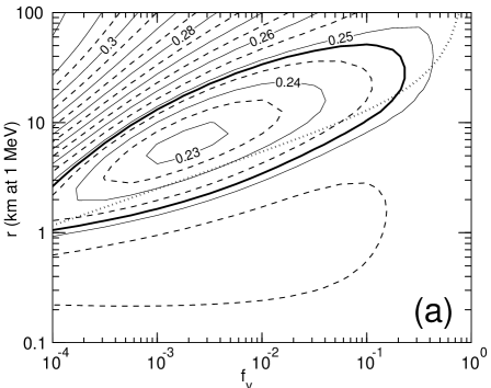
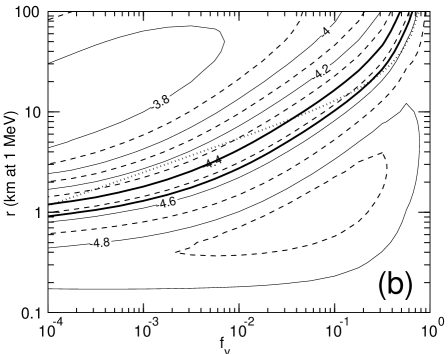
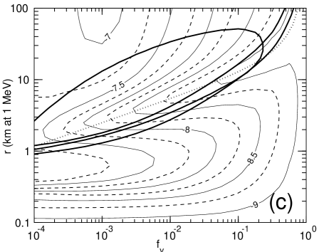
FIG. 1.: The light element yields (a) $Y_{p}$, (b) $\log_{10}({\rm D}/{\rm H})$, and (c) $\log_{10}({}^{7}{\rm Li}/{\rm H})$ as a function of the high-density volume fraction $f_{v}$ and the distance scale $r$, for the CC (centrally condensed) geometry and $\omega_{b}=0.030$. The density contrast $R$ is fixed by $f_{v}R=100$. The observational limits $Y_{p}\leq 0.248$ and ${\rm D}/{\rm H}=2.9$–$4.0\times 10^{-5}$ are indicated by thick lines (both are shown superposed on the ${}^{7}{\rm Li}$ yield in (c)). The dotted line shows the $r(f_{v})$ relation, “optimum valley”, chosen for Fig. 3. The limit of small $r$ or large $f_{v}$ gives the SBBN result.

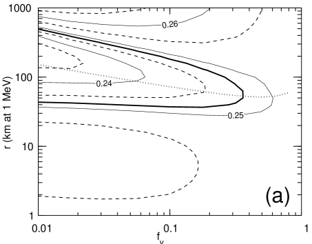
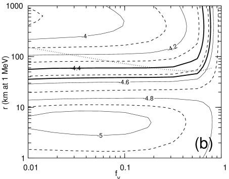
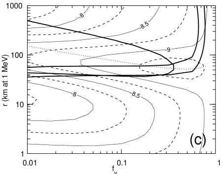
FIG. 2.: Same as Fig. 1, but for the SS (spherical shell) geometry. The dotted line shows the $r(f_{v})$ relation, “optimum valley”, chosen for Fig. 4.

It has been customary in IBBN work to choose $R$ sufficiently large to get rid of the $R$-dependence. This reduces the dimension of the parameter space by one, and maximizes the effect of the inhomogeneity. We first follow this practice by fixing $f_{v}R=100$, and show the IBBN yields of ${}^{4}{\rm He}$, ${\rm D}$, and ${}^{7}{\rm Li}$ in the remaining two dimensional parameter space $(f_{v},r)$ in Fig. 1 for the CC geometry, and in Fig. 2 for the SS geometry.

All our distances given in km refer to comoving distance at $T=$ 1 MeV. Note that 1 km at 1 MeV corresponds to 8.5 m at 100 MeV and to $1.9\times 10^{-4}$ pc today.

We see that IBBN leads to acceptable ${}^{4}{\rm He}$ and ${\rm D}$ yields for $\omega_{b}=0.030$. This occurs for distance scales which are near the “optimum distance scale” for IBBN. Moreover, choosing the “high” observed value for $Y_{p}$, and the “low” observed value for ${\rm D}/{\rm H}$ gives us agreement for moderate (not very small) values of $f_{v}$, where the ${}^{7}{\rm Li}$ yield is the lowest. Choosing a lower $Y_{p}$ and a higher ${\rm D}/{\rm H}$ would move the agreement towards smaller $f_{v}$, where the ${}^{7}{\rm Li}$ yield would be significantly larger than in SBBN. However, for the SS geometry, somewhat higher ${\rm D}/{\rm H}$ values would be fine.

For SBBN with $\omega_{b}=0.030$, all three observables, $Y_{p}$, ${\rm D}/{\rm H}$, and ${}^{7}{\rm Li}/{\rm H}$ are outside their observed ranges. While the inhomogeneity at the right distance scale had the effect of moving $Y_{p}$ and ${\rm D}/{\rm H}$ into the observed range, this is not true for ${}^{7}{\rm Li}/{\rm H}$. For the CC geometry IBBN does not reduce the ${}^{7}{\rm Li}$ yield appreciably. For the SS geometry there is a reduction in ${}^{7}{\rm Li}/{\rm H}$ for not too small $f_{v}$, which could arguably be sufficient.

To see what the effect of the remaining parameter, $R$ has on this lithium problem, we choose to track the “lithium valley” of Figures 1 and 2. In[33] we derived the dependence of the optimum scale $r_{\rm opt}$ on $f_{v}$ and $\eta$,

$$r_{\rm opt} \propto {f_{v}^{1/3}\over(1-f_{v})}\eta^{-2/3}\qquad\hbox{(CC)}$$ (2)

$$r_{\rm opt} \propto {\eta^{-2/3}\over f_{v}^{1/3}(1-f_{v})^{1/3}}\qquad\hbox{(SS)}.$$ (3)

From Figures 1 and 2, we see that the minimum ${}^{7}{\rm Li}$ yield occurs for slightly smaller distance scales than the minimum ${}^{4}{\rm He}$ yield. We choose the proportionality constant so that $r(f_{v})$ tracks the low ${}^{7}{\rm Li}$ yields. Thus we have taken

$$r = 25{\rm km}{f_{v}^{1/3}\over(1-f_{v})}\qquad\hbox{(CC)}$$ (4)

$$r = 32.5{\rm km}{1\over f_{v}^{1/3}(1-f_{v})^{1/3}}\qquad\hbox{(SS)},$$ (5)

(the dotted lines in Figures 1 and 2). We now allow $R$ to vary independently of $f_{v}$ and show the results in Figures 3 and 4.

To check that the lithium valley does not shift in $r$ as the density contrast $R$ is reduced, we repeated this for nearby distance scales.

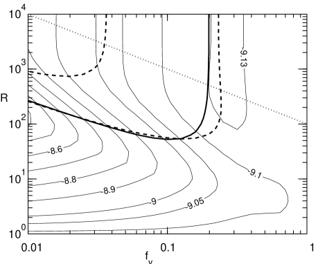
FIG. 3.: The lithium yield, $\log_{10}({}^{7}{\rm Li}/{\rm H})$, as a function of the high-density volume fraction $f_{v}$ and the density contrast $R$ for the CC geometry. The distance scale $r$ corresponds to the dotted line in Fig. 1. The observational limits $Y_{p}\leq 0.248$ (above the solid line) and ${\rm D}/{\rm H}=2.9$–$4.0\times 10^{-5}$ (between the dashed lines) are indicated by thick lines. The dotted line corresponds to the relation $f_{v}R=100$ used for Fig. 1. Taking $R=1$ or $f_{v}=1$ gives the SBBN result. To bring out the slight decrease in the${}^{7}{\rm Li}/{\rm H}$ yield, we have included the $\log_{10}({}^{7}{\rm Li}/{\rm H})=-9.13$ contour in this figure.

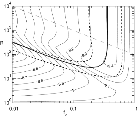
FIG. 4.: Same as Fig. 3, but for the SS geometry.

These figures quantify the effect of the density contrast $R$ in IBBN. We see how the effect indeed saturates for $f_{v}R\gtrsim 100$. For IBBN to have the desired effect of bringing $Y_{p}$ and ${\rm D}/{\rm H}$ into agreement with observations for a high baryon density (here $\omega_{b}=0.03$), we need a density contrast of $R\gtrsim 4/f_{v}$. Varying $R$ does not have much effect on the lithium problem. The smallest ${}^{7}{\rm Li}$ yield we get with acceptable $Y_{p}$ and ${\rm D}/{\rm H}$ is ${}^{7}{\rm Li}/{\rm H}=7.4\times 10^{-10}$ for the CC geometry and ${}^{7}{\rm Li}/{\rm H}=4.0\times 10^{-10}$ for the SS geometry.

We found that IBBN with the CC geometry is not able to reduce the ${}^{7}{\rm Li}$ yield significantly, but the SS geometry can reduce it by about a factor of two. Thus one could argue for a marginal IBBN case, where we have an initial inhomogeneity approximating the SS geometry, i.e., the surface-to-volume ratio of the high-density regions is relatively large. With a high-density volume fraction $f_{v}=0.2$–$0.5$, density contrast $R>30$, and a distance scale $r=35$–$70$ km at 1 MeV, we get $Y_{p}$ near the upper limit 0.248, ${\rm D}/{\rm H}$ comfortably in the observed primordial range, and ${}^{7}{\rm Li}/{\rm H}\sim 4\times 10^{-10}$. With the uncertainties in the ${}^{7}{\rm Li}/{\rm H}$ observations and BBN reaction rates leading to ${}^{7}{\rm Li}$ this is in agreement with observations if one is willing to accept a depletion factor of about two.

We are, however, not aware of a well-motivated scenario for producing a baryon inhomogeneity both with this geometry and this distance scale in the early universe.

A baryon inhomogeneity could be generated during inflation as an isocurvature perturbation, or after inflation in some phase transition. In the latter case, the distance scale must be less than the horizon size during the phase transition. At the electroweak phase transition, the horizon size is about 3 km, and the expected distance scale is significantly smaller than this, too small to have a large effect on BBN[33].

The QCD transition is the most studied candidate for generating the inhomogeneity for IBBN[32]. The horizon size at the QCD transition is about 2000 km. In a first-order transition, the resulting baryon density contrast could well be large enough, and the distribution of distance scales[36] would be fairly narrow. In homogeneous thermal nucleation, the distance scale depends on the latent heat $L$ and the surface tension $\sigma$ of the phase transition. Typical estimates from lattice QCD calculations[37] give distance scales which are much too small for our scenario, although combinations of $L$ and $\sigma$ leading to sufficiently large distance scales may not be completely ruled out[38]. Heterogeneous nucleation due to impurities could also lead to larger distance scales, of about 1 km[39]. (Note that in the literature these distances are often quoted as comoving at 100 MeV, and thus smaller by a factor of 1/117).

Because of primordial perturbations the nucleation of the phase transition does not take place in homogeneous conditions. The cosmic fluid is undergoing acoustic oscillations at subhorizon scales. Since the nucleation rate is extremely sensitive to the temperature, thermal nucleation would occur only at cold spots. This could lead to a distance scale of the order of 1 km[40], which is large enough to affect nucleosynthesis. However, the inhomogeneities produced by the QCD transition appear likely to resemble the CC geometry more than the SS geometry.

III Conclusions

It is intriguing, that the “high” baryon density $\omega_{b}\sim 0.03$, suggested by recent CMB results fits so well with the “low” ${\rm D}/{\rm H}$ and “high” $Y_{p}$ observations in the IBBN scenario. However, the ${}^{7}{\rm Li}$ yield is significantly higher than the standard estimates for its primordial value.

For the SS geometry, IBBN can reduce the lithium yield by about a factor of two in the best case, but for $\omega_{b}=0.03$, we still get ${}^{7}{\rm Li}/{\rm H}=4\times 10^{-10}$, requiring depletion by at least a factor of two in the Spite plateau. This may be marginally acceptable, especially if one allows for the uncertainty in the ${}^{7}{\rm Li}$ yield due to the reaction rates.

We note for comparison, that the widely accepted “low-D” determination $\omega_{b}=0.020$ in SBBN yields ${}^{7}{\rm Li}/{\rm H}=3.4\times 10^{-10}$ and thus also requires significant lithium depletion[41].

The better developed scenarios for producing the kind of inhomogeneity needed for IBBN tend to lead to the CC type of geometry. For this geometry, IBBN is not able to reduce the lithium abundance significantly below the SBBN result, so that depletion by a factor of four would be needed. This seems to be considered unacceptable at present.

REFERENCES

- [1] Electronic address: Hannu.Kurki-Suonio@helsinki.fi
- [2] Electronic address: Elina.Sihvola@helsinki.fi
- [3] D.N. Schramm and R.V. Wagoner, Ann. Rev. Nucl. Sci. 27, 37 (1977); D.N. Schramm and M.S. Turner, Rev. Mod. Phys. 70, 303 (1998); K.A. Olive, Eur. Phys. J. C15, 133 (2000) (Review of Particle Physics).
- [4] M. Kaplinghat and M.S. Turner, astro-ph/0007454.
- [5] P. de Bernardis et al., Nature (London) 404, 955 (2000).
- [6] S. Hanany et al., astro-ph/0005123.
- [7] A.E. Lange et al., astro-ph/0005004; A. Balbi et al., astro-ph/0005124; A.H. Jaffe et al., astro-ph/0007333; J.R. Bond et al., astro-ph/0011378.
- [8] S. Burles, K.M. Nollett, and M.S. Turner, astro-ph/0008495.
- [9] K.A. Olive and G. Steigman, Astrophys. J. Supp. S. 97, 49 (1995); K.A. Olive, G. Steigman, and E.D. Skillman, Astrophys. J. 483, 788 (1997). M. Peimbert, A. Peimbert, and M.T. Ruiz, astro-ph/0003154, have recently measured in the Small Magellanic Cloud, and based on this, estimate .
- [10] Y.I. Izotov, T.X. Thuan, and V.A. Lipovetsky, Astrophys. J. 435, 647 (1994); Astrophys. J. Supp. S. 108, 1 (1997); Y.I. Izotov and T.X. Thuan, Astrophys. J. 500, 188 (1998).
- [11] K.A. Olive, astro-ph/0009475.
- [12] S. Burles and D. Tytler, Astrophys. J. 499, 699 (1998); ibid. 507, 732 (1998). J.M. O’Meara, D. Tytler, D. Kirkman, N. Suzuki, J.X. Prochaska, D. Lubin, and A.M. Wolfe, astro-ph/0011179, have recently added a fourth detection, and revised the combined estimate to and .
- [13] J.K. Webb, R.F. Carswell, K.M. Lanzetta, R. Ferlet, M. Lemoine, A. Vidal-Madjar, and D.V. Bowen, Nature (London) 388, 250 (1997).
- [14] S.A. Levshakov, W.H. Kegel, and F. Takahara, Astrophys. J. Lett. 499, L1 (1998); Astron. Astrophys. 336, 29L (1998); Mon. Not. R. Astron. Soc. 302, 707 (1999).
- [15] K.A. Olive, G. Steigman, and T.P. Walker, Phys. Rep. 333-334, 389 (2000); D. Tytler, J.M. O’Meara, N. Suzuki, and D. Lubin, Physica Scripta, T85, 12 (2000), astro-ph/0001318.
- [16] G. Steigman, astro-ph/0009506.
- [17] M. Spite and F. Spite, Astron. Astrophys. 115, 357 (1982); Nature (London) 297, 483 (1982).
- [18] P. Bonifacio and P. Molaro, Mon. Not. R. Astron. Soc. 285, 847 (1997).
- [19] M.H. Pinsonneault, T.P. Walker, G. Steigman, and V.K. Narayanan, Astrophys. J. 527, 180 (1999).
- [20] S.G. Ryan, T.C. Beers, C.P. Deliyannis, and J.A. Thorburn, Astrophys. J. 458, 543 (1996); S.G. Ryan, J.E. Norris, and T.C. Beers, Astrophys. J. 523, 654 (1999).
- [21] S.G. Ryan, T.C. Beers, K.A. Olive, B.D. Fields, and J.E. Norris, Astrophys. J. Lett. 530, L57 (2000). Using the data of [20], T.K. Suzuki, Y. Yoshii, and T.C. Beers, Astrophys. J. 540, 99 (2000), estimate a primordial abundance .
- [22] S. Vauclair and C. Charbonnell, Astron. Astrophys. 295, 715 (1995); Astrophys. J. 502, 372 (1998).
- [23] C. Deliyannis, talk at IAU Symposium 198, Natal (Brazil) 1999.
- [24] M. White, D. Scott, and E. Pierpaoli, astro-ph/0004385; M. Tegmark and M. Zaldarriaga, Phys. Rev. Lett. 85, 2240 (2000).
- [25] K. Enqvist, H. Kurki-Suonio, and J. Väliviita, Phys. Rev. D 62, 103003 (2000).
- [26] J. Barriga, E. Gaztañaga, M.G. Santos, and S. Sarkar, astro-ph/0011398.
- [27] F.R. Bouchet, P. Peter, A. Riazuelo, and M. Sakellariadou, astro-ph/0005022.
- [28] map.gsfc.nasa.gov/.
- [29] astro.estec.esa.nl/Planck/.
- [30] R.A. Malaney and G.J. Mathews, Phys. Rep. 229, 145 (1993); S. Sarkar, Rep. Prog. Phys. 59, 1493 (1996); H. Kurki-Suonio, astro-ph/0002071.
- [31] J. Lesgourgues and M. Peloso, Phys. Rev. D 62, 081301 (2000); M. Orito, T. Kajino, G.J. Mathews, and R.N. Boyd, astro-ph/0005446; S. Esposito, G. Mangano, G. Miele, and O. Pisanti, J. High Energy Phys. 9, 038 (2000); S. Esposito, G. Mangano, A. Melchiorri, G. Miele, and O. Pisanti, astro-ph/0007419; P. Di Bari and R. Foot, hep-ph/0008258.
- [32] J.H. Applegate, C.J. Hogan, and R.J. Scherrer, Phys. Rev. D 35, 1151 (1987); H. Kurki-Suonio, R.A. Matzner, J.M. Centrella, T. Rothman, and J.R. Wilson, Phys. Rev. D 38, 1091 (1988); G.J. Mathews, B.S. Meyer, C.R. Alcock, and G.M. Fuller, Astrophys. J. 358, 36 (1990). Refs. [30, 33] contain a more extensive set of references.
- [33] K. Kainulainen, H. Kurki-Suonio, and E. Sihvola, Phys. Rev. D 59, 083505 (1999).
- [34] C. Angulo et al.(The NACRE collaboration), Nucl. Phys. A656, 3 (1999).
- [35] E. Vangioni-Flam, A. Coc, and M. Cassé, astro-ph/0002248.
- [36] B.S. Meyer, C.R. Alcock, G.J. Mathews, and G.M. Fuller, Phys. Rev. D 43, 1079 (1991).
- [37] QCDPAX collaboration, Y. Iwasaki et al., Phys. Rev. D 46, 4657 (1992); B. Grossmann and M.L. Laursen, Nucl. Phys. B408, 637 (1993); Y. Iwasaki, K. Kanaya, L. Kärkkäinen, K. Rummukainen, and T. Yoshié, Phys. Rev. D 49, 3540 (1994).
- [38] J. Ignatius, K. Kajantie, H. Kurki-Suonio, and M. Laine, Phys. Rev. D 50, 3738 (1994).
- [39] M.B. Christiansen and J. Madsen, Phys. Rev. D 53, 5446 (1996).
- [40] J. Ignatius and D.J. Schwarz, hep-ph/0004259.
- [41] S. Burles, K.M. Nollett, and M.S. Turner, astro-ph/0010171.