The effects of vertical outflows on disk dynamos

We consider the effect of vertical outflows on the mean-field dynamo in a thin disk. These outflows could be due to winds or magnetic buoyancy. We analyse both two-dimensional finite-difference numerical solutions of the axisymmetric dynamo equations and a free-decay mode expansion using the thin-disk approximation. Contrary to expectations, a vertical velocity can enhance dynamo action, provided the velocity is not too strong. In the nonlinear regime this can lead to super-exponential growth of the magnetic field.

1 Introduction

Magnetic fields play an important role in accretion disks. Inside the disk, for example, they allow the magneto-rotational instability to develop (Balbus & Hawley 1998). This instability can lead to the development of turbulence which in turn transports angular momentum radially outwards, thus allowing the matter to accrete. On the other hand, large scale magnetic fields are often considered necessary for launching winds or jets from accretion disks. The origin of such large scale magnetic fields is still unclear: they may be advected from the surrounding medium or be generated by a dynamo inside the disk. Advection appears unlikely as turbulence leads to enhanced viscosity and magnetic diffusivity, so that the two are of the same order (Prandtl number of order unity; Pouquet et al. 1976). Thus, turbulent magnetic diffusivity can compensate the dragging of the field by viscously induced accretion flow (van Ballegooijen 1989; Lubow et al. 1994; Heyvaerts et al. 1996). Dynamo action is a plausible mechanism for producing magnetic fields in accretion disks (Pudritz 1981; Stepinski & Levy 1988). However, dynamo magnetic fields can affect winds from accretion disks (Campbell et al. 1998; Campbell 1999; Brandenburg et al. 2000). On the other hand, the wind can also affect the dynamo. In particular, an enhancement by wind was suggested by Brandenburg et al. (1993) in the context of galactic dynamos. In the same context, Elstner et al. (1995) also consider the effects of shear in the wind.

In this paper, we consider the generation of magnetic field by a dynamo acting in a thin accretion disk. We provide a study of the effects of vertical velocities. We show how vertical velocities can enhance the dynamo, allowing a larger growth rate and leading to super-exponential growth of the magnetic field in the nonlinear regime.

The vertical velocities considered can have several origins. They can, for example, be due to a wind emanating from the disk or to magnetic buoyancy inside the disk. Note that we are interested here in magnetic buoyancy as generating vertical outflows. We neglect the associated dynamo effect (Moss et al. 1999).

The paper is organized as follows. In Sect. 2, we describe the two complementary approaches used and specify our choice of parameters. In Sect. 3, we discuss the linear results without vertical outflows. Results with vertical outflows are discussed in Sect. 4 for the linear regime and in Sect. 5 for the nonlinear regime. Sect. 6 presents our conclusions.

2 The models

Simulations of dynamo-generated turbulence in accretion disks have shown that, if stratification is included, a large scale field can be generated whose structure and dependence on boundary conditions closely resemble what is known from mean-field $\alpha\omega$-dynamo theory (Brandenburg 1998). It has been suggested that nonlinear effects can suppress the $\alpha$-effect to insignificant values (Vainshtein & Cattaneo 1992), but as recent simulations have shown, this does not affect the very possibility of mean-field dynamo action, but merely the time-scale on which the large scale field is established (Brandenburg 2001). With these justifications in mind, we adopt the mean-field approximation. The evolution of the magnetic field is given by

$$\frac{\partial\@vec{B}}{\partial t}=\@vec{\nabla}\times(\@vec{V}\times\@vec{B}+\alpha\@vec{B}-\eta\@vec{\nabla}\times\@vec{B}),$$ (1)

where $\eta$ is the turbulent magnetic diffusivity and $\alpha$ the coefficient quantifying the $\alpha$-effect. We ignore anisotropies of $\alpha$ because only the toroidal diagonal component of the $\alpha$-tensor matters in the so-called $\alpha\Omega$-regime. The antisymmetric part of the $\alpha$-tensor corresponds to turbulent diamagnetism which tends to push magnetic fields into the disk, and therefore just lowers the effective wind speed. Furthermore, as shown by Gabov et al. (1996, Fig. 6), turbulent diamagnetism is relatively unimportant for dynamo numbers less than 200, and our results mostly refer to this range. Given the substantial uncertainties in the mean-field transport coefficients, we decided to adopt the simplest possible approach. In order to minimize the number of parameters in our model, we also neglect the radial component of the velocity and thus our velocity field is $\@vec{V}=(0,r\Omega,V_{z})$ in cylindrical coordinates ($r,\varphi,z$) (see comments in Sect. 2.2 on the consequences of this assumption).

We use two approaches to solve this equation. Firstly, a 2D numerical simulation based on a finite-difference scheme is applied (Sect. 2.1). Secondly, we develop a 1D free-decay mode expansion (Sect. 2.2). Details of these two complementary approaches are given below. Each of these two methods has its own advantages. The finite-difference simulation allows investigation of the nonlinear behaviour and applies to 2D geometry. On the other hand, the free-decay mode expansion gives the full eigenstructure and provides a tool for qualitative analysis. Furthermore, boundary conditions corresponding to an ideal vacuum can be implemented easily in the 1D model, whereas our 2D model where the disk is embedded in a halo can provide only an approximation to a vacuum outside the disk. Our two approaches are therefore complementary.

The problem is governed by three dimensionless numbers which appear in the dimensionless form of Eq. (1). Let $h$, the half-thickness of the disk, be a characteristic length-scale, $\alpha_{0}$ a characteristic value of $\alpha$, $V_{z0}$ a characteristic vertical velocity and $\eta_{0}$ a characteristic value of $\eta$. We also define the rotational shear $S(r)=r\mathrm{d}\Omega/\mathrm{d}r$. The dimensionless numbers are the azimuthal magnetic Reynolds number

$$R_{\omega}=\frac{Sh^{2}}{\eta_{0}},$$ (2)

the magnetic Reynolds number based on the $\alpha$-effect

$$R_{\alpha}=\frac{\alpha_{0}h}{\eta_{0}},$$ (3)

and the vertical magnetic Reynolds number

$$R_{v}=\frac{V_{z0}h}{\eta_{0}}.$$ (4)

Note that $\alpha_{0}$ and $S$ depend on $r$ and thus the magnetic Reynolds numbers $R_{\omega}$ and $R_{\alpha}$ also depend on $r$. However, we assume later that $\alpha_{0}S$ is approximately constant. In this work, we adopt the $\alpha\omega$-approximation for the dynamo. In that case, for thin disks, the growth rates depend on the dynamo number $\cal D\equiv R_{\alpha}R_{\omega}$ only and not on the individual values of $R_{\alpha}$ and $R_{\omega}$. However, note that the ratio of the radial to the azimuthal magnetic field $|B_{r}|/|B_{\varphi}|$ is about $\sqrt{|R_{\alpha}|/|R_{\omega}|}$ (Ruzmaikin et al. 1988). Moreover, Pudritz (1981) showed that the dynamo number $\cal D$ is approximately constant in a thin accretion disk.

2.1 The finite-difference model

To ensure that the magnetic field $\@vec{B}$ is solenoidal, we evolve the induction equation in terms of the vector potential $\@vec{A}$, where $\@vec{B}=\@vec{\nabla}\times\@vec{A}$,

$${\partial\@vec{A}\over\partial t}=\@vec{V}\times\@vec{B}+\alpha\@vec{B}-\eta\mu_{0}\@vec{j},$$ (5)

where $\@vec{j}=\@vec{\nabla}\times\@vec{B}/\mu_{0}$ is the current density due to the mean magnetic field and $\mu_{0}$ is the magnetic permeability. The $\alpha$-term $\alpha\@vec{B}$ together with the velocity term $\@vec{V}\times\@vec{B}$ drives the mean-field dynamo. We restrict ourselves to axisymmetric solutions of Eq. (5). We do not make the thin-disk approximation in this model but we consider thin disks by choosing an appropriate aspect ratio (see below). We do not make the $\alpha\omega$-dynamo assumption explicitly i.e. we retain the $\alpha$-effect in the equations for $A_{r}$ and $A_{z}$, but we restrict ourselves to the $\alpha\omega$-dynamo regime by our choice of magnetic Reynolds numbers $|R_{\omega}|/|R_{\alpha}|=10^{4}\mbox{--}10^{6}$.

Our computational domain contains the disk embedded in a halo: $0\leq r\leq L_{r}{=}2$, $|z|\leq L_{z}{=}1$, where the disk occupies the region $0\leq r\leq 1.5$, $|z|\leq 0.15$, $R=1.5$ being the outer radius of the disk and $h=0.15$ its half-thickness. This results in a disk aspect ratio of $h/R=0.1$ and the upper boundary of the domain at $z\simeq 7h$. Using a resolution of $101\times 101$ grid points and a uniform grid, the resulting mesh spacing is $\delta r=\delta z=0.02$. Equation (5) is solved using a sixth order finite-difference scheme in space and a third order Runge–Kutta time advance scheme.

We control the symmetry of our solutions (dipolar or quadrupolar) by using appropriate initial conditions. On the boundaries of the computational domain (i.e. far away from the disk) we impose the conditions that the normal component of $\@vec{A}$, $A_{\perp}$, vanishes together with the normal derivative of the tangential components, $\@vec{A}_{\parallel}$,

$$A_{\perp}=0,\quad{\partial\over\partial n}\@vec{A}_{\parallel}=0.$$ (6)

This is similar to the “normal-field” condition, where the tangential components of the magnetic field and the normal component of the electric field $\@vec{E}$ vanish, $\@vec{B}_{\parallel}=\@vec{0}$, $E_{\perp}=0$. To verify that the boundary conditions do not affect our results, we have also tried perfectly conducting boundary conditions and found differences in the magnetic field structure only in the close vicinity of the boundaries.

The $\alpha$-coefficient $\alpha(r,z)$ is antisymmetric about the midplane and vanishes outside the disk. We adopt

$$\alpha(r,z)=\left\{\begin{array}[]{cl}\alpha_{0}(r)\sin(\pi z/h)&\mbox{for $|z|\leq h$},\\ 0&\mbox{for $|z|>h$}.\end{array}\right.$$ (7)

The radial profile of $\alpha(r,z)$ is smoothly cut off at $r>R$ and at $r_{i}=0.15$ where the rotational shear is very strong.

As appropriate for accretion disks, we adopt a softened Keplerian angular velocity profile in $r$ in the whole computational domain (including the halo as well as the disk), assuming $\Omega$ to be $z$-independent:

$$\Omega(r)=\sqrt{GM\over r^{3}}\left[1+\left({r_{0}\over r}\right)^{n}\right]^{-{(n+1)/2n}},$$ (8)

where $G$ is Newton’s gravitational constant, $M$ the mass of the central object, $r_{0}=0.05$ the softening radius, and $n=5$. At $r=0$, $\Omega$ vanishes as $r^{3/2}$.

The turbulent magnetic diffusivity is given by an interpolation between $\eta_{\rm disk}$ in the disk midplane and $\eta_{\rm halo}$ in the halo,

$$\eta(r,z)=\eta_{\rm halo}+(\eta_{\rm disk}-\eta_{\rm halo})\xi(r,z).$$ (9)

Here, the profile $\xi(r,z)$ defines the disk,

$$\xi(r,z)=g(r-r_{0},d)\,g(|z|-z_{0},d),$$ (10)

where $g(x,d)$ is a smoothed Heaviside step function with a smoothing half-width $d$ set to 8 grid zones. So $\xi(r,z)$ is equal to unity deep in the disk and vanishes in the halo.

To obtain the magnetic Reynolds numbers of Eqs. (2)–(4) we choose $\eta_{0}=\eta_{\rm disk}$.

In accretion disks, the dynamo number is approximately constant with radius. In this model this is achieved by setting

$$\alpha_{0}(r)={{\cal D}\eta_{\rm disk}^{2}\over S(r)h^{3}}.$$ (11)

2.2 The free-decay mode expansion

The lowest order approximation for Eq. (1) in a thin disk results from retaining derivatives with respect to $z$ alone. In the $\alpha\omega$-approximation and with a constant $\eta$, Eq. (1) then becomes (see Ruzmaikin et al. (1988) for a form with $V_{z}=0$)

$$\frac{\partial B_{r}}{\partial t} = -\frac{\partial}{\partial z}(\alpha B_{\varphi})+\eta\frac{\partial^{2}B_{r}}{\partial z^{2}}-\frac{\partial}{\partial z}(V_{z}B_{r}),$$ (12)

$$\frac{\partial B_{\varphi}}{\partial t} = SB_{r}+\eta\frac{\partial^{2}B_{\varphi}}{\partial z^{2}}-\frac{\partial}{\partial z}(V_{z}B_{\varphi}),$$ (13)

where once again $S(r)=rd\Omega/dr$ and where $B_{r}$ and $B_{\varphi}$ are respectively the radial and azimuthal components of the magnetic field. Note that we have neglected $V_{r}$, the radial component of the velocity in the disk, but the inclusion of this extra term would be straightforward (Moss et al. 2000).

We consider solutions with exponential time dependence

$$B_{r}(z,t) = \widetilde{B_{r}}(z)\;\exp(\gamma t),$$ (14)

$$B_{\varphi}(z,t) = \widetilde{B_{\varphi}}(z)\;\exp(\gamma t),$$ (15)

where $\gamma$ is the complex growth rate. Measuring $z$ in units of the half-thickness $h$ of the disk, $t$ in units of the diffusion time $h^{2}/\eta$, the coefficient $\alpha$ in units of a characteristic value $\alpha_{0}$ and $V_{z}$ in units of a characteristic value $V_{z0}$, the dimensionless form of Eq. (12) and Eq. (13) is given by

$$\gamma\widetilde{B_{r}} = -R_{\alpha}\frac{\mathrm{d}}{\mathrm{d}z}(\alpha\widetilde{B_{\varphi}})+\frac{\mathrm{d}^{2}\widetilde{B_{r}}}{\mathrm{d}z^{2}}-R_{v}\frac{\mathrm{d}}{\mathrm{d}z}(V_{z}\widetilde{B_{r}}),$$ (16)

$$\gamma\widetilde{B_{\varphi}} = R_{\omega}\widetilde{B_{r}}+\frac{\mathrm{d}^{2}\widetilde{B_{\varphi}}}{\mathrm{d}z^{2}}-R_{v}\frac{\mathrm{d}}{\mathrm{d}z}(V_{z}\widetilde{B_{\varphi}}),$$ (17)

where we have kept the same notation for the dimensionless variables and where $R_{\omega}$, $R_{\alpha}$ and $R_{v}$ are given by Eqs. (2), (3) and (4) with $\eta_{0}=\eta$.

We expand $\widetilde{B_{r}}$ and $\widetilde{B_{\varphi}}$ with respect to the orthonormal base formed by the free-decay modes (Galerkin expansion),

$$\widetilde{B_{r}}=\sum_{n=0}^{N}a_{n}B_{r}^{0,n}\>,\qquad\widetilde{B_{\varphi}}=\sum_{n=0}^{N}b_{n}B_{\varphi}^{0,n},$$ (18)

where $a_{n}$ and $b_{n}$ are complex coefficients. The free-decay modes are the solutions of the equation

$$\gamma_{n}^{0}\@vec{B}^{0,n}=\frac{\mathrm{d}^{2}}{\mathrm{d}z^{2}}\@vec{B}^{0,n}.$$ (19)

Vacuum boundary conditions are imposed at the disk surface. We impose them for each free-decay mode so that $\widetilde{B_{r}}$ and $\widetilde{B_{\varphi}}$, and thus $B_{r}$ and $B_{\varphi}$, satisfy these conditions

$$B_{r}^{0,n}|_{z=1}=B_{\varphi}^{0,n}|_{z=1}=0.$$ (20)

At the midplane, the boundary conditions are connected to the symmetry of the mode considered. For quadrupolar modes we have

$$\left.\frac{\mathrm{d}B_{r}^{0,n}}{\mathrm{d}z}\right|_{z=0}=\left.\frac{\mathrm{d}B_{\varphi}^{0,n}}{\mathrm{d}z}\right|_{z=0}=0,$$ (21)

and for dipolar modes we have

$$B_{r}^{0,n}|_{z=0}=B_{\varphi}^{0,n}|_{z=0}=0.$$ (22)

Thus, the normalized eigenfunctions of free decay and the corresponding growth rates are, for quadrupolar symmetry

$$B_{r,\varphi}^{0,n} = \sqrt{2}\cos\left(\left({\textstyle{1\over 2}}+n\right)\pi z\right)\>\>\>\>\mathrm{with}\>\>n=0,1\ldots N,$$ (23)

$$\gamma_{n}^{0} = -\left({\textstyle{1\over 2}}+n\right)^{2}\pi^{2},$$ (24)

and for dipolar symmetry

$$B_{r,\varphi}^{0,n} = \sqrt{2}\sin(n\pi z)\>\>\>\>\mathrm{with}\>\>n=0,1\ldots N,$$ (25)

$$\gamma_{n}^{0} = -n^{2}\pi^{2}.$$ (26)

Note that the free-decay dipolar mode $n=0$ would correspond to a uniform steady vertical magnetic field. The free-decay modes are normalized such that

$$\int_{0}^{1}{\left(B_{r,\varphi}^{0,n}\right)^{2}}\mathrm{d}z=1$$ (27)

(except for the dipolar mode with $n=0$). The free-decay modes are degenerate, forming doublets $(B_{r}^{0,n},0),(0,B_{\varphi}^{0,n})$ decaying at the same rate $\gamma_{n}^{0}$.

After making this expansion, the differential equations become an algebraic set of equations forming an eigenvalue problem of $2(N+1)$ equations

$$(\gamma-\gamma_{m}^{0})a_{m} = -R_{\alpha}\sum_{n=0}^{N}b_{n}Y_{nm}-R_{v}\sum_{n=0}^{N}a_{n}W_{nm}^{r},$$ (28)

$$(\gamma-\gamma_{m}^{0})b_{m} = R_{\omega}a_{m}-R_{v}\sum_{n=0}^{N}b_{n}W_{nm}^{\varphi},$$ (29)

with $m=0,1\ldots N$.

The coefficients $W_{nm}^{r}$, $W_{nm}^{\varphi}$ and $Y_{nm}$ are defined by

$$W_{nm}^{r} = \int_{0}^{1}B_{r}^{0,m}(V_{z}\;B_{r}^{0,n})^{\prime}\,\mathrm{d}z,$$ (30)

$$W_{nm}^{\varphi} = \int_{0}^{1}B_{\varphi}^{0,m}(V_{z}\;B_{\varphi}^{0,n})^{\prime}\,\mathrm{d}z,$$ (31)

$$Y_{nm} = \int_{0}^{1}B_{r}^{0,m}(\alpha B_{\varphi}^{0,n})^{\prime}\,\mathrm{d}z,$$ (32)

where the prime denotes the derivative with respect to $z$. We normalize the eigenfunctions (18) such that

$$\int\limits_{0}^{1}\left[\left(\frac{\widetilde{B_{r}}}{R_{\alpha}}\right)^{2}\!\!\!\!+\widetilde{B_{\varphi}}^{2}\right]\mathrm{d}z=\sum_{n=0}^{N}\left[\left(\frac{|a_{n}|}{R_{\alpha}}\right)^{2}\!\!\!\!+|b_{n}|^{2}\right]=1.$$ (33)

In this model, the truncation level needed depends on the values of $R_{v}$ and $\cal D$. Typically, $N=4$ is enough to compute the eigenvalues (growth rates) of the problem whereas $N=9$ is usually required to compute the eigenfunctions. The precision of all the results presented here was checked.

2.3 Choice of parameters

In this section, we discuss properties that are common to the two models.

The rotation of the thin disk is assumed to be close to Keplerian and independent of $z$ for the finite-difference model (see Sect. 2.1). Only the assumption of the independence of $\Omega$ on $z$ is needed in the free-decay mode expansion.

We use two configurations: one where the magnetic diffusivity is the same in the disk and in the halo around the disk ($\eta_{\mathrm{halo}}=\eta_{\mathrm{disk}}$) and one with a low conductivity in the halo or a vacuum around the disk. Note that assuming a vacuum or low conductivity in the halo above the disk is a rather good approximation for galaxies (Sokoloff & Shukurov 1990; Poezd et al. 1993). It also allows for a connection with established theory. Note finally that the low-conductivity approximation ($\@vec{j}\approx\@vec{0}$) is a good approximation for potential fields ($\@vec{j}=\@vec{0}$) and hence for a particular case of force-free fields ($\@vec{j}\times\@vec{B}=\@vec{0}$).

The boundary conditions of the free-decay mode expansion imply a vacuum above the disk. Technically, to achieve $\eta_{\mathrm{halo}}=\eta_{\mathrm{disk}}$ in this model, we restrict the dynamo action to an inner layer of the disk. The outer part of the disk is thus playing the role of the halo. The results simply need to be rescaled for a proper comparison.

In the finite-difference model, we study the case $\eta_{\mathrm{halo}}=\eta_{\mathrm{disk}}$ and the case of a low conductivity halo with $\eta_{\mathrm{halo}}/\eta_{\mathrm{disk}}=20$. Note that, with this model, to approximate a vacuum in the halo we have to choose $\eta_{\mathrm{halo}}/\eta_{\mathrm{disk}}$ as high as possible. But, this choice is restricted because the higher this ratio, the smaller the time step.

In this paper, the model with $\eta_{\mathrm{halo}}=\eta_{\mathrm{disk}}$ is referred to as the “disk+halo” model whereas the model with a vacuum or low conductivity above the disk is referred to as the “disk+vacuum” model.

In both models, the profile for $\alpha$ is taken to be

$$\alpha=\alpha_{0}\sin\left(\pi\frac{z}{h}\right)\>\>\mbox{for}\>\>|z|\leq h$$ (34)

(see Eq. (7) for details concerning the finite-difference model), except in Fig. 1 where we take a linear dependence of $\alpha$ with $z$ to compare with previous work. The profile for $V_{z}$ is linear in $z$,

$$V_{z}=V_{z0}\frac{z}{h}.$$ (35)

The accuracy of the models depends on the number of grid points in $r$ and $z$ for the finite-difference model and on the level of truncation for the free-decay mode expansion.

In this work, the two control parameters are the dynamo number $\cal D$ and the vertical magnetic Reynolds number $R_{v}$. For reference, we give here possible values for these two parameters. While dynamo numbers are rather low in galactic disks, $|{\cal D}|\lesssim 10$ (Ruzmaikin et al. 1988), in accretion disks, they can be as high as $|{\cal D}|\simeq 10^{2}-10^{4}$, depending on the Mach number of the turbulence, see e.g. Pudritz (1981). The value of $R_{v}$ obviously depends on the origin of the vertical outflow. With magnetic buoyancy, a rough estimate can be obtained assuming that the vertical motions occur at the Alfvén speed. Estimating the Alfvén speed from magnetic equipartition, one gets a vertical magnetic Reynolds number $R_{v}$ of order unity.

In the following, the figures obtained with the finite-difference model are labelled with “FD” and the ones obtained with the free-decay mode (Galerkin) expansion with “GE”.

3 Linear results for $R_{v}=0$

In this section, we present results with no vertical velocity in the disk ($R_{v}=0$). Such a study is an interesting test for the quality of the results of the free-decay mode expansion. It also gives a point of comparison between the numerical simulation and the free-decay mode expansion.

We first compare the results of the free-decay mode expansion (with $R_{v}=0$) with the results published by Stepinski & Levy (1991). We thus take a linear dependence of $\alpha$ on $z$, $\alpha=\alpha_{0}z/h$. The calculated growth rates are plotted in Fig. 1. The agreement is good but a discrepancy is observed at large $|\cal D|$ where the increase of the growth rate with $|\cal D|$ is faster according to Stepinski & Levy than in our free-decay mode expansion for both quadrupolar and dipolar symmetry (${\cal D}<0$). This discrepancy seems to be due to an insufficient number of grid points in Stepinski & Levy’s model. Indeed, if we increase the truncation level of the free-decay mode expansion, no change is observed in the results whereas if we decrease the truncation level, we recover the results of Stepinski & Levy. Note that the results discussed in this paper are for $|{\cal D}|<400$ where the agreement is excellent.

We now want to compare the finite-difference simulation with the free-decay mode expansion. In particular, we want to test our method to mimic, in the case of the free-decay mode expansion, a model for $\eta_{\mathrm{halo}}=\eta_{\mathrm{disk}}$ starting with the “disk+vacuum” model (see Sect. 2). For an infinitely extended halo with $\eta_{\mathrm{halo}}=\eta_{\mathrm{disk}}$, the growth rates of dipolar and quadrupolar modes should be exchanged when $\cal D$ reverses sign, i.e. the graph of $Re(\gamma)$ as a function of $\cal D$ should be symmetric with respect to the vertical axis (Proctor 1977). The finite-difference simulation shows this symmetry with a good precision (Fig. 2a). The results of the free-decay mode expansion (Fig. 2b) are less symmetric. This is not surprising since the ratio between the height of the computational domain and the height of the disk is about 7 in the finite-difference simulation whereas it is only 2 in the free-decay mode expansion.

Figure 1: Real part of the growth rate of the magnetic field as a function of $|{\cal D}|$, with $\alpha=\alpha_{0}z/h$, obtained with the free-decay-mode expansion with $N\geq 9$. Asterisks denote non-oscillatory solutions whereas diamonds denote oscillatory solutions. Solid lines are for quadrupolar modes and dotted lines for dipolar modes. Signs above the curves indicate the sign of ${\cal D}$.

We now discuss our results for the “disk+halo” and “disk+vacuum” configuration. Let us first consider the “disk+halo” configuration (Figs. 2a and b). For moderate dynamo number $|{\cal D}|\lesssim 300$, the leading mode is quadrupolar and non-oscillatory if ${\cal D}<0$ ($R_{\alpha}>0$) and it is dipolar and non-oscillatory if ${\cal D}>0$ ($R_{\alpha}<0$). In the following, we thus study the effect of vertical motions for ${\cal D}<0$ in quadrupolar symmetry and for ${\cal D}>0$ in dipolar symmetry. Above $|{\cal D}|\simeq 300$, the symmetry of the leading mode changes and it becomes oscillatory. The critical dynamo number is $|{\cal D}_{\rm crit}|\simeq 5$.

Let us now consider the “disk+vacuum” configuration (Figs. 2c and d). The results obtained with the two approaches are rather different. With the free-decay mode expansion, the dipolar mode is always oscillatory and subcritical for $|{\cal D}|\leq 400$. On the other hand, with the finite-difference simulation, the dipolar mode becomes supercritical for ${\cal D}\gtrsim 50$ and is non-oscillatory for all ${\cal D}>0$. This is because the dominant dipolar mode in the finite-difference simulation is the “forgotten mode” i.e. a dipolar mode corresponding to $n=0$ in Eqs. (25) and (26). The “forgotten mode” cannot be obtained with our 1D calculation (free-decay mode expansion). However, we reproduced the corresponding profile $\gamma({\cal D})$ with a modified 1D model which takes into account the finite aspect ratio of the disk. The model is based on the assumption of separability of $r$- and $z$-dependence and yields equations similar to the thin-disk equations (12), (13), but with additional correction terms of order $(h/r)^{2}$. Thus, the dipolar modes of Fig. 2c and Fig. 2d are of a different nature. As for the quadrupolar mode, the results obtained with the two approaches are not so different. The branch for ${\cal D}<0$ is rather similar in both cases with a critical dynamo number $\gtrsim-50$. The branch for ${\cal D}>0$ is all subcritical with the finite-difference simulation whereas it becomes supercritical for ${\cal D}\sim 170$ with the free-decay mode expansion. However, we have checked that, in the finite-difference model, if we take a steeper transition between $\eta_{\mathrm{disk}}$ and $\eta_{\mathrm{halo}}$, the branch for ${\cal D}>0$ moves upwards, resembling the one for the free-decay mode expansion.

The qualitative behaviour for the case of low conductivity in the halo is in many respects similar to that of the “disk+halo” configuration (Figs. 2a and c). But there are quantitative differences. There is no intersection point where the symmetry of the leading mode would change for $|{\cal D}|\lesssim 700$. The diagram does not look symmetric anymore.

The results of the finite-difference model presented here are in agreement with the accretion disk models of Rüdiger et al. (1995) and von Rekowski et al. (2000). Note, however, that these models have an inner radius and that at this radius a perfectly conducting boundary condition is used, which leads to a vertical current layer on the boundary and potentially lowers the excitation threshold for magnetic fields.

Figure 2: a-d Real part of the growth rate of the magnetic field as a function of $-{\cal D}$ for $R_{v}=0$. Asterisks denote non-oscillatory solutions and diamonds denote oscillatory solutions. Solid lines indicate quadrupolar modes and dashed lines indicate dipolar modes. a and c are for the finite-difference model (FD) and b and d are for the free-decay mode expansion model (GE) with a and b for the “disk+halo” model and c and d for the “disk+vacuum” model. Note the approximate symmetry of graphs a and b with respect to the vertical axis. Note also that the dipolar mode in c is the “forgotten mode”, not seen in d.

4 Linear behaviour with vertical velocities

In this section, we study the linear behaviour of the $\alpha\omega$-dynamo in the presence of vertical velocity ($R_{v}\neq 0$). As discussed in Sect. 3, we present results for quadrupolar symmetry with ${\cal D}<0$ (Sect. 4.1) and results for dipolar symmetry with ${\cal D}>0$ (Sect. 4.2.). An explanation of these results is given in Sect. 4.3.

4.1 Quadrupolar modes

We consider quadrupolar modes with ${\cal D}<0$. For sufficiently low dynamo numbers ($|{\cal D}|\lesssim 50$), the growth rate decreases with $R_{v}$ whereas at larger dynamo numbers, the growth rate increases for small $R_{v}$ and then decreases at large $R_{v}$, forming a maximum (Fig. 3). This maximum is a robust feature, the existence of which does not seem to depend on the boundary conditions or on the model. Indeed, we find this maximum with the finite-difference simulation (Figs. 3a and c) and with the free-decay mode expansion (Figs. 3b and d) in both configurations, “disk+halo” and “disk+vacuum” (see Sect. 2.3 for the definition of these configurations). The boundary conditions at the surfaces of the disk affect the position of the maximum in $R_{v}$ and the dynamo number above which it occurs. In particular, the smaller the magnetic diffusivity of the halo, the smaller this dynamo number. Nevertheless, the required values for $\cal D$ to get a maximum are larger than the typical values in galaxies. When ${\cal D}$ is increased, the maximum is more pronounced and its position is shifted towards larger $R_{v}$. Note that the values of $R_{v}$ at which the maximum occurs are between 1 and 10. They thus fit within the range of values estimated for magnetic buoyancy. Finally, in the range of dynamo numbers studied here, $|{\cal D}|\lesssim 300$, the vertical velocity does not change the symmetry or temporal behaviour of the dominant mode.

Figure 3: a-d Real part of the growth rate of the magnetic field as a function of $R_{v}$ for the dominant quadrupolar mode and for different dynamo numbers. All modes are non-oscillatory. a and c are for the finite-difference model (FD) and b and d are for the free-decay mode expansion model (GE) with a and b for the “disk+halo” model and c and d for the “disk+vacuum” model. The models of panels a to d correspond to the ones in Fig. 2.

We now discuss the magnetic field structure. Figure 4 shows the eigenfunctions for $B_{r}$ and $B_{\varphi}$ for ${\cal D}=-200$ and for different $R_{v}$ in the “disk+halo” configuration. With this choice of the dynamo number, a maximum in the curve $\gamma(R_{v})$ occurs around $R_{v}=7.5$. An obvious feature is that the vertical velocity pushes the zeros of $B_{r}$ and $B_{\varphi}$ outwards. For the dynamo to work, it is essential that $B_{r}$ changes sign in the disk since only then can magnetic flux of the opposite sign to that in the midplane leave through the disk surface (Ruzmaikin et al. 1988). When $R_{v}$ takes large values, the radial component of the magnetic field $B_{r}$ has no zero inside the disk and thus the dynamo cannot work ($\gamma<0$). This is the technical reason for the decrease of $\gamma$ with $R_{v}$. The physical reason for it is investigated in Sect. 4.3. The increase of the growth rate at small $R_{v}$ will be explained in Sect. 4.3. We note however that when we decrease the truncation level of the free-decay mode expansion down to $N=0$ (one doublet), the maximum disappears.

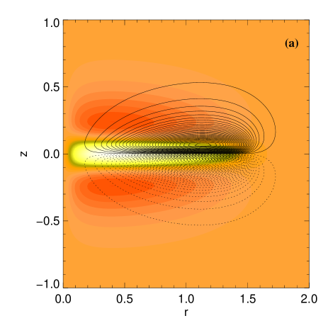
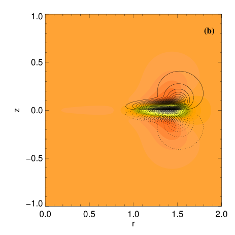
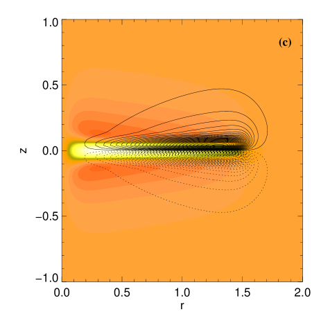
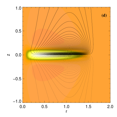
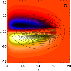
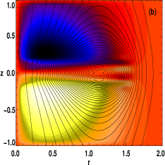
The magnetic field configuration in 2D geometry is shown in Fig. 5. It shows both the effect of increasing the dynamo number and the effect of increasing the vertical magnetic Reynolds number. When one decreases the dynamo number from ${\cal D}=-50$ to ${\cal D}=-200$, in the absence of any vertical velocity, the magnetic field becomes more concentrated at the outer edge of the disk (Figs. 5a and 5b). If the vertical magnetic Reynolds number is then increased from $R_{v}=0$, the magnetic field is radially redistributed over the whole disk (Fig. 5c) and then advected towards the halo (Fig. 5d). From panel (b) to (d), the growth rate increases as shown by the curve for ${\cal D}=-200$ in Fig. 3a. Thus, the magnetic field diffusion becomes less efficient as the vertical scale of the magnetic field increases with $R_{v}$. This leads to an increase of the growth rate up towards its maximum at $R_{v}=7.5$ (Fig. 5d). Note that in the halo the poloidal magnetic field lines become more and more aligned with lines of constant angular velocity as $R_{v}$ increases. Note also that the mode structure of Fig. 5d (where Re($\gamma$) is maximum for ${\cal D}=-200$) is very similar to the mode structure for $-{\cal D}=50,R_{v}=3$, where that mode has attained its maximum growth rate.

Figure 4: a-d Vertical structure of the non-oscillatory quadrupolar magnetic field for ${\cal D}=-200$. Panels a and c are for the finite-difference model (FD) while panels b and d are for the free-decay mode expansion (GE). Panels a and b give the radial structure and c and d give the azimuthal structure of the magnetic field. In the finite-difference model, eigenfunctions are taken at $r=1$ and are normalized such that $\max|B_{\varphi}|=1$ for each $R_{v}$. Note that in the free-decay mode expansion, we plot $\widetilde{B_{r}}$ and $\widetilde{B_{\varphi}}$, i.e. the time-independent part of the magnetic field.

Figure 5: a-d Magnetic field configuration obtained using the finite-difference model with the linear “disk+halo” configuration and for the dominant non-oscillatory quadrupolar mode. Contours represent poloidal magnetic field lines with solid lines being clockwise and dotted lines being counter-clockwise. The greyscales are the intensity and direction of the azimuthal magnetic field; light grey (dark grey) signifies $B_{\varphi}>0$ ($B_{\varphi}<0$). The parameters are a ${\cal D}=-50$, $R_{v}=0$, b ${\cal D}=-200$, $R_{v}=0$, c ${\cal D}=-200$, $R_{v}=0.75$, d ${\cal D}=-200$, $R_{v}=7.5$ (where Re$(\gamma)$ is maximum). Comparing a and b shows the effect of increasing the dynamo number. b–d show the effect of increasing $R_{v}$.

4.2 Dipolar modes

We now study the linear behaviour with vertical velocity for positive ${\cal D}$ where the dipolar non-oscillatory mode is dominant. Figure 6 shows that there is no maximum in the growth rates; at $R_{v}$ of order $1$ or even less the dynamo is switched off.

The magnetic field structure in 2D geometry is shown in Fig 7. The magnetic field structures for ${\cal D}=50$ and $R_{v}=0$ and $0.75$ show that the field is advected vertically outwards and the poloidal field lines are aligned with the $\Omega$ contours lines very quickly.

Figure 6: Real part of the growth rate of the magnetic field as a function of $R_{v}$ for the dominant dipolar mode and for different dynamo numbers in the “disk+halo” model. Asterisks denote non-oscillatory modes whereas diamonds denote oscillatory ones.

Figure 7: a and b. Magnetic field configuration obtained using the finite-difference model with the linear “disk+halo” configuration and for the dominant non-oscillatory dipolar mode. The parameters are a ${\cal D}=50$, $R_{v}=0$, b ${\cal D}=50$, $R_{v}=0.75$. The notation is the same as in Fig. 5.

4.3 The origin of the dynamo enhancement

In this section, we explain why a vertical velocity can increase the growth rate of the dynamo. Therefore, we plot the different terms of Eq. (16) and Eq. (17) obtained with the free-decay mode expansion. To avoid any ambiguity with the choice of normalization, in particular when comparing results at different $R_{v}$, we rewrite the equations in the following way. We multiply Eq. (16) and Eq. (17) by $B_{r}$ and $B_{\varphi}$ respectively, and we integrate over the disk thickness. We thus obtain

$$\gamma=\gamma_{\alpha}^{r}+\gamma_{\mathrm{diff}}^{r}+\gamma_{\mathrm{stret}}^{r},$$ (36)

$$\gamma=\gamma_{\omega}^{\varphi}+\gamma_{\mathrm{diff}}^{\varphi}+\gamma_{\mathrm{stret}}^{\varphi},$$ (37)

with

$$\gamma_{\alpha}^{r} = -R_{\alpha}\frac{\int_{0}^{1}B_{r}(\alpha B_{\varphi})^{\prime}\mathrm{d}z}{\int_{0}^{1}B_{r}^{2}\mathrm{d}z},$$ (38)

$$\gamma_{\omega}^{\varphi} = R_{\omega}\frac{\int_{0}^{1}B_{r}B_{\varphi}\mathrm{d}z}{\int_{0}^{1}B_{\varphi}^{2}\mathrm{d}z},$$ (39)

$$\gamma_{\mathrm{diff}}^{r,\varphi} = \frac{\int_{0}^{1}B_{r,\varphi}B_{r,\varphi}^{\prime\prime}\mathrm{d}z}{\int_{0}^{1}B_{r,\varphi}^{2}\mathrm{d}z}=-\frac{\int_{0}^{1}\left(B_{r,\varphi}^{\prime}\right)^{2}\mathrm{d}z}{\int_{0}^{1}B_{r,\varphi}^{2}\mathrm{d}z},$$ (40)

$$\gamma_{\mathrm{stret}}^{r,\varphi} = -R_{v}\frac{\int_{0}^{1}B_{r,\varphi}(V_{z}B_{r,\varphi})^{\prime}\mathrm{d}z}{\int_{0}^{1}B_{r,\varphi}^{2}\mathrm{d}z}-\frac{R_{v}}{2}\frac{\int_{0}^{1}V_{z}^{\prime}B_{r,\varphi}^{2}\mathrm{d}z}{\int_{0}^{1}B_{r,\varphi}^{2}\mathrm{d}z},$$ (41)

where we have used a vacuum boundary condition at $z=h$ to rewrite $\gamma_{\mathrm{stret}}$, $\gamma_{\mathrm{diff}}$. This form of the equations allows us to investigate the different physical contributions to the growth rate $\gamma$. Note that Eqs. (36) and (37) are not explicitly time-dependent. The terms $\gamma_{\alpha}^{r}$ and $\gamma_{\omega}^{\varphi}$ are the contributions to the growth rate $\gamma$ from the $\alpha$-effect and $\omega$-effect. The terms $\gamma_{\mathrm{diff}}^{r,\varphi}$ are the contributions from dissipation which are always negative. Finally, the terms $\gamma_{\mathrm{stret}}^{r,\varphi}$ are the contributions to $\gamma$ from stretching the magnetic field. The profile for $V_{z}$ is always antisymmetric with respect to the disk midplane and $V_{z}^{\prime}>0$ for $z>0$. Thus, these stretching terms $\gamma_{\mathrm{stret}}^{r,\varphi}$ are always negative. In particular, with a linear profile for $V_{z}$, they are both equal to $-R_{v}/2$.

The general picture is as follows. The positive contribution to $\gamma$ comes from $\gamma_{\alpha}^{r}$ and $\gamma_{\omega}^{\varphi}$ whereas dissipation has a negative contribution. In the presence of a vertical velocity, an additional negative contribution comes from the stretching of the magnetic field $\gamma_{\mathrm{stret}}^{r,\varphi}$. But, at the same time, the stretching reduces dissipation by increasing the scale of the magnetic field (see Eq. (40)). Thus, depending on the relative values of the reduction of dissipation and of the negative stretching term, the growth rate is enhanced or not (a maximum occurs or not). Obviously, when the magnetic field is completely stretched, dissipation cannot be reduced anymore. However, this does not necessarily correspond to the maximum of the growth rate as the terms $\gamma_{\alpha}^{r}$ and $\gamma_{\omega}^{\varphi}$ evolve themselves with $R_{v}$ (which quantifies the vertical velocity). These different quantities are plotted in Fig. 8 in a case where a maximum occurs and in a case with no maximum.

We note that dissipation increases again after being reduced by the stretching of the magnetic field in the vertical direction. This increased dissipation is due to the formation of boundary layers near $z=h$. We also note that the term $\gamma_{\alpha}^{r}$ decreases whereas $\gamma_{\omega}^{\varphi}$ increases. The evolution of these terms is linked to the disappearance of the positive area of $B_{r}$ (with the convention of sign of Fig. 4). Finally, note that at large $R_{v}$, the growth rate $\gamma$ always decreases as the stretching terms $\gamma_{\mathrm{stret}}^{r,\varphi}$ become dominant.

Figure 8: a-d Contributions of the different terms in Eqs. (36) and (37) to the growth rate $\gamma$ in the “disk+vacuum” model. Lines are labelled with the subscripts used for the different terms in Eqs. (36) and (37). a and c represent the radial and azimuthal terms for ${\cal D}=-200$, for which a maximum occurs, b and d represent the radial and azimuthal terms for ${\cal D}=-10$, for which no maximum occurs.

In short, the growth rate can increase with $R_{v}$, thus forming a maximum, because dissipation is reduced by the stretching of the magnetic field.

5 Nonlinear behaviour with vertical velocities

The nonlinear behaviour has only been investigated with the finite-difference model. We restrict ourselves here to the model “disk+halo” ($\eta_{\rm halo}=\eta_{\rm disk}$) and to negative dynamo numbers considering only quadrupolar symmetry which, for $R_{v}=0$, is the dominant symmetry for moderate values of ${\cal D}<0$. Solutions are all saturated and non-oscillatory, as in the corresponding linear modes. We study three different cases of nonlinearity: magnetic buoyancy, $\alpha$-quenching and a combination of both. For a comparison of nonlinear solutions with a different parametrization of magnetic buoyancy see earlier works by Torkelsson & Brandenburg (1994a, b).

5.1 Magnetic buoyancy

We parameterize the effect of magnetic buoyancy by assuming that the vertical velocity depends on the horizontal magnetic field,

$$V_{z}(z)=V_{z0}\,\frac{z}{h}\,\sqrt{B_{r}^{2}+B_{\varphi}^{2}}/B_{\rm eq},$$ (42)

where $B_{\rm eq}$ is the equipartition magnetic field $B_{\rm eq}=\sqrt{\rho\mu_{0}}c_{\mathrm{s}}{\rm Ma}_{\rm turb}$, $\rho$ is the density, $c_{\mathrm{s}}$ the sound speed and ${\rm Ma}_{\rm turb}$ a turbulent Mach number, treated here as a free parameter. The profiles of density $\rho$ and sound speed $c_{\mathrm{s}}$ are taken from a simple model of a cool accretion disk embedded in a hot corona (Brandenburg et al. 2000; see also Dobler et al. 1999).

We define an effective vertical magnetic Reynolds number

$$R_{v}^{\rm(eff)}=R_{v}\,\left\langle\sqrt{B_{r}^{2}+B_{\varphi}^{2}}/B_{\rm eq}\right\rangle_{\rm disk},$$ (43)

where $\langle\cdot\rangle_{\mathrm{disk}}$ denotes averaging over the disk. Fig. 9 shows the magnetic energy and $R_{v}^{\rm(eff)}$ as a function of time for ${\cal D}=-200$ and $R_{v}=7.5$. This value of $R_{v}$ corresponds to the location of the maximum of the growth rate $\gamma(R_{v})$ in the linear model (cf. Fig. 3a, upper curve). Starting from an initial magnetic field strength $B_{\rm init}=10^{-5}$, $\@vec{B}$ grows and therefore $R_{v}^{\rm(eff)}$ increases; so the growth rate roughly follows the upper curve in Fig. 3a. Thus, as long as $R_{v}^{\rm(eff)}$ is approximately less than the position of the maximum of $\gamma$, i.e. the horizontal magnetic field is smaller than the equipartition field, $\gamma$ increases with time, which results in the super-exponential growth of the magnetic energy seen for $10\lesssim t\lesssim 28$ (Fig. 9). After $t\approx 28$, when the horizontal field is comparable with the equipartition field, $\gamma$ decreases and eventually the magnetic field approaches its saturation level. This level is reached when $R_{v}^{\rm(eff)}\simeq R_{v*}\approx 21.5$, where $R_{v*}$ is the zero of $\gamma(R_{v})$ in Fig. 3a, upper curve.

Figure 9: Magnetic energy and effective vertical magnetic Reynolds number $R_{v}^{\rm(eff)}$ as a function of time for the “disk+halo” model with magnetic buoyancy (cf. Eq. (42)). ${\cal D}=-200$ and $R_{v}=7.5$. Super-exponential growth occurs before saturation sets in. The mode is quadrupolar and non-oscillatory. The initial magnetic field strength is $B_{\rm init}=10^{-5}$. The steep increase for $t\lesssim 2$ is due to the generation of azimuthal field from the initial large scale poloidal one at the chosen high $R_{\omega}$.

In this subsection we assume that the only nonlinearity is due to magnetic buoyancy and thus appears in the vertical velocity term only. In particular, we do not consider here any dependence of $\alpha$ or $\eta$ on $\@vec{B}$. In this case the dimensionless form of the induction equation in the steady state reads

$$\hat{\cal L}\@vec{B}+\@vec{\nabla}\times\left[\left(R_{v}\,\sqrt{B_{r}^{2}+B_{\varphi}^{2}}/B_{\rm eq}\right)\,\@vec{u}\times\@vec{B}\right]=0,$$ (44)

where $\hat{\cal L}$ is a linear operator and $u$ is a vector function of position, $\@vec{u}=(0,0,z/h)$ in the case considered here. Let $\@vec{b}$ be the solution of Eq. (44) for $R_{v}=1$. Then, for arbitrary $R_{v}$, the solution is $\@vec{b}/R_{v}$. From this, it follows that the saturation value of magnetic energy is

$$E_{\mathrm{mag}}^{\mathrm{sat}}={1\over R_{v}^{2}}E_{\mathrm{mag}}^{\mathrm{sat}}\Bigr{|}_{R_{v}=1}\propto{1\over R_{v}^{2}},$$ (45)

and the structure of the saturated magnetic field is independent of $R_{v}$. This is confirmed with our numerical model.

The magnetic field is extended into the whole halo and almost completely stretched. Therefore, adding a wind term such that

$$V_{z}(z)=\left(V_{z0}^{\rm buoy}\,\sqrt{B_{r}^{2}+B_{\varphi}^{2}}/B_{\rm eq}+V_{z0}^{\rm wind}\right)\frac{z}{h}$$ (46)

and fixing $R_{v}^{\rm buoy}=R_{v}^{\rm(eff)}$ while increasing $R_{v}^{\rm wind}=R_{v}$, cannot lead to enhancement of magnetic energy. The wind is carrying magnetic field away and $E_{\rm mag}$ is decreasing.

5.2 $\alpha$-quenching

We now parameterize the back-reaction of the magnetic field on the turbulent $\alpha$-effect by making $\alpha$ depend on $\@vec{B}$,

$$\alpha(r,z)=\alpha_{0}(r)\sin\left(\pi\frac{z}{h}\right){\xi_{\alpha}(r)\over 1+{B^{2}/B_{\rm eq}^{2}}},$$ (47)

where $B_{\rm eq}$ is again the equipartition magnetic field.

Figure 10: Magnetic energy as a function of $R_{v}$ for the “disk+halo” model with $\alpha$-quenching. All modes are quadrupolar and non-oscillatory.

Figure 11: a-c Magnetic field configuration for the “disk+halo” model with $\alpha$-quenching: the effect of vertical velocity. Poloidal field (lines) and azimuthal field (grey scales). a ${\cal D}=-50$, $R_{v}=0$; b ${\cal D}=-50$, $R_{v}=3$; c ${\cal D}=-50$, $R_{v}=7.5$. a-c following the lower curve in Fig. 10. All modes are quadrupolar and non-oscillatory.

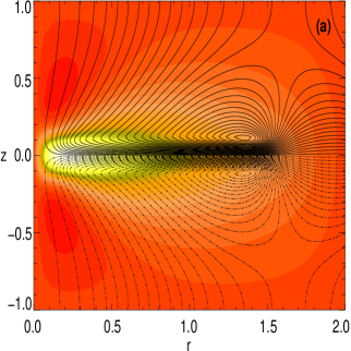
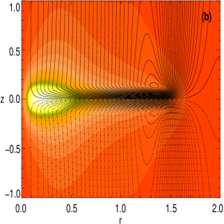
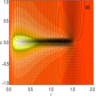
Figure 10 shows the magnetic energy as a function of $R_{v}$ for the three dynamo numbers ${\cal D}=-50$, ${\cal D}=-100$ and ${\cal D}=-200$. From this we can see the following features:

• $E_{\rm mag}$ has a maximum as a function of $R_{v}$ in the nonlinear regime;

• but, this maximum is shifted towards much smaller $R_{v}$ (of order $0.1$), compared to that of the growth rate in the linear regime, and it is also less pronounced;

• the value of $R_{v}$ where the maximum in $E_{\rm mag}$ occurs, is almost independent of ${\cal D}$;

• the magnetic energy scales roughly with the dynamo number, $E_{\rm mag}\propto{\cal D}$;

• all modes remain non-oscillatory when increasing $R_{v}$.

The effect of vertical velocity on the structure of the magnetic field for the model with $\alpha$-quenching can be seen in Fig. 11 where it is shown for ${\cal D}=-50$. But looking at the magnetic field configuration for ${\cal D}=-100$ and ${\cal D}=-200$, one finds that the field structure changes only weakly with the dynamo number.

5.3 $\alpha$-quenching together with magnetic buoyancy

In this section, we combine $\alpha$-quenching, Eq. (47), with magnetic buoyancy, Eq. (42), and compare the results with the case of $\alpha$-quenching with wind. In Fig. 12, magnetic energy is plotted against $R_{v}^{({\rm eff})}$ for these two models and for ${\cal D}=-50$. Evidently, the two curves behave similarly, supporting the notion that wind and magnetic buoyancy have similar effects on the dynamo. For $R_{v}^{({\rm eff})}\ll 1$, the field structure is solely determined by $\alpha$-quenching and thus $E_{\rm mag}$ is independent of $R_{v}^{({\rm eff})}$. For $R_{v}^{({\rm eff})}\gg 1$, on the other hand, $\alpha$-quenching becomes unimportant and $E_{\rm mag}\propto(R_{v}^{({\rm eff})})^{-2}$, as discussed in Sect. 5.1. The largest disagreement between the two curves occurs for intermediate values of $R_{v}^{({\rm eff})}$, i.e. where both $\alpha$-quenching and magnetic buoyancy are important, and where the field has not yet reached its asymptotic shape (Fig. 11c).

Perfect agreement between the two curves cannot be expected, because the averaging in Eq. (43) was somewhat arbitrary; the agreement could perhaps be improved by choosing a different definition of $R_{v}^{({\rm eff})}$. The fact that with magnetic buoyancy the magnetic energies are larger for a given value of $R_{v}^{({\rm eff})}$ can therefore not be interpreted as a relative enhancement of dynamo action.

Figure 12: Magnetic energy as a function of $R_{v}^{\rm(eff)}$ defined in Eq. (43) for the models with $\alpha$-quenching with wind and $\alpha$-quenching combined with magnetic buoyancy. $\eta_{\rm halo}=\eta_{\rm disk}$ and ${\cal D}=-50$. All modes are quadrupolar and non-oscillatory. With $\alpha$-quenching alone, $R_{v}^{\rm(eff)}=R_{v}$.

6 Conclusions

Disk dynamos have been studied intensively over the past 20 years, but only recently the effects of outflows and winds have been included (e.g. Campbell 1999; Dobler et al. 1999; Brandenburg et al. 2000). It was immediately clear that these changes in the boundary conditions affect the structure of the solutions. The present work is an attempt to provide a more thorough survey of solutions with wind for different values and sign of the dynamo number. One of the effects that we have highlighted is the enhancement of the kinematic dynamo growth rate for intermediate strengths of the wind. In the nonlinear case this corresponds to a phase shortly before saturation where the growth becomes super-exponential.

In the present work we have deliberately isolated the dynamo problem from the wind problem. In reality the two aspects together constitute a more complicated self-consistent dynamo problem that needs to be looked at in more detail in future. One step in that direction was taken by Brandenburg et al. (2000) where the feedback on the flow from the Lorentz force was taken fully into account. A more formidable task would be to obtain self-consistent dynamo action in three dimensions without assuming an $\alpha$-effect, thus obtaining dynamo action and outflows in a self-consistent manner from first principles. In the context of accretion disks, this would require simulating turbulent dynamo action, where the turbulence itself is driven by dynamo-generated magnetic fields (Brandenburg et al. 1995). This would be of great interest not only from the astrophysical point of view, but also from that of dynamo theory in general, because, as was recently realized, the catastrophic quenching of the standard $\alpha\omega$-dynamo could be alleviated in the presence of open boundary conditions which may substantially improve the working of the dynamo (Blackman & Field 2000). This is simply because the $\alpha$-effect generates helical fields, but at the same time magnetic helicity is conserved in a closed domain. Thus, being able to get rid of helical fields through open boundaries may be vital for the dynamo (Brandenburg & Dobler 2001). Furthermore, the production of fields at large scales could be facilitated by the production – and subsequent loss through boundaries – of small scale fields with opposite sign of magnetic helicity. This latter aspect could not be addressed with mean-field models and would require a direct simulation of accretion disk turbulence in a global model.