Star Formation History and Stellar Metallicity Distribution in a $\Lambda$ Cold Dark Matter Universe

Abstract

We study star formation history and stellar metallicity distribution in galaxies in a $\Lambda$ cold dark matter universe using a hydrodynamic cosmological simulation. Our model predicts star formation rate declining in time exponentially from an early epoch to the present with the time-scale of 6 Gyr, which is consistent with the empirical Madau plot with modest dust obscuration. Star formation in $L^{*}$ galaxies continues intermittently to the present also with an exponentially declining rate of a similar time-scale, whereas in small galaxies star formation ceases at an early epoch. The mean age of the extant stars decreases only slowly with increasing redshift, and exceeds $1{\rm\,Gyr}$ at $z=3$. Normal galaxies contain stars with a wide range of metallicity and age: stars formed at $z<1$ have metallicity of $0.1-1.0Z_{\odot}$, while old stars take a wide range of values from $10^{-6}Z_{\odot}$ to $3.0Z_{\odot}$. The mean metallicity of normal galaxies is in the range $0.1-1.0Z_{\odot}$. Dwarf galaxies that contain only old stars have a wide range of mean metallicity ($10^{-4}-1.0Z_{\odot}$), but on average they are metal deficient compared with normal galaxies.

1. Introduction

Over the last 15 years, cold dark matter (CDM) models have served as basic frameworks to study the formation of cosmic structure, and have been successful in delineating a scenario of galaxy formation (Davis et al., 1985; Blumenthal et al., 1984). We now understand the formation of large-scale structure reasonably well in terms of a CDM model dominated by a cosmological constant $\Lambda$ (Efstathiou, Sutherland, & Maddox, 1990; Ostriker and Steinhardt, 1995; Turner and White, 1997; Balbi et al., 2000; Lange et al., 2000; Hu, et al., 2000).

When and how galaxies formed, however, are a far more complicated problem due to non-gravitational physical processes operating on small scales. Many authors use semianalytic models to study galaxy formation, where dark matter halo formation under the hierarchical structure formation is supplemented heuristically with physical processes for baryons (White & Frenk, 1991; Baugh et al., 1998; Kauffmann et al., 1999a; Somerville and Primack, 1999; Cole et al., 2000). They have succeeded to give a picture of galaxy formation roughly consistent with observations, but have the disadvantage that one has to assume a set of simplified model equations, often associated with additional free parameters, for each physical process included in the model. The advantage of semianalytic models is, on the other hand, that they are computationally light, and therefore, one can search for a viable model with a small amount of cost.

An alternative but computationally much more expensive approach is direct cosmological hydrodynamic simulations. So far, intergalactic medium and overall galaxy formation processes have been well studied with hydrodynamic approach (e.g., Cen and Ostriker, 1992a, 1993, 2000; Katz, Weinberg, & Hernquist, 1996) (see Pearce et al., 1999, however). Much effort invested in improving the accuracy of simulations has brought the hydrodynamic mesh approaching to $(1000)^{3}$, with which we may hope that we obtain meaningful results on some aspects of galaxy properties. It is certainly impossible to resolve internal structure of galaxies with the present simulations. Nevertheless, we would expect that global properties such as global star formation rate (SFR) are described reasonably well with a few adjustable parameters, since they primarily depend on thermal balance of the bulk of clouds, such as how gas cools, or how surrounding gas is reheated by feedback by star formation. The fact that we obtain a reasonable amount of baryonic mass frozen into stars and a global metal abundance with reasonable input parameters justifies, at least in part, our expectation.

In this paper, we primarily discuss the star formation history of galaxies and the evolution of stellar metallicity, which are the direct output of the simulation. The aspects that require additional use of a stellar population synthesis model, such as luminosity function and colors of galaxies, will be discussed in a separate publication Nagamine, Fukugita, Cen, and Ostriker (2001, hereafter Paper II). Since the hydrodynamic approach is computationally demanding, we do not attempt to make a fine tuning of input parameters, but our aim here instead is to make qualitative predictions which can be used to either verify or falsify the $\Lambda$CDM model by future observations with only a limited number of assumptions, treating the dynamics of baryons more accurately than in semianalytic models.

Our results would give insight on how galaxies are assembled from an early epoch to the present. Observationally interesting questions would include: (i) How old are stars in normal and dwarf galaxies, and what is their age distribution? A relevant question is whether star formation takes place continuously or intermittently; (ii) What is the stellar metallicity distribution in normal and dwarf galaxies? A relevant old problem is the paucity of metal poor stars in the solar neighborhood (G-dwarf problem: van den Bergh, 1962; Schmidt, 1963); (iii) Is there a unique age-metallicity relation for stars in normal galaxies, and (iv) Is there a relation between the mass of galaxies and average metallicity? How these aspects evolve with redshift is also an observationally relevant problem, although the observational studies could answer only for global properties for high-redshift objects. Our simulation yield unambiguous predictions to these problems, at least qualitatively.

In § 2, we describe our simulation. In § 3 we first present the global star formation history of the entire simulation box. We then discuss in § 4 the star formation history of individual galaxies. The mean age of the stars and the formation epoch of galaxies are discussed in § 5. We discuss the stellar metallicity distribution and the mean metallicity of galaxies in § 6, and conclude in § 7.

2. Simulation and Parameters

We use a recent Eulerian hydrodynamic cosmological simulation with a comoving box size of 25$h^{-1}$ Mpc with $768^{3}$ grid cells and $384^{3}$ dark matter particles of mass $2.03\times 10^{7}h^{-1}{\,\,M_{\odot}}$. The comoving cell size is $32.6h^{-1}$ kpc, and the mean baryonic mass per cell is $3.35\times 10^{5}h^{-1}M_{\odot}$ ($h$ is the Hubble constant in units of $H_{0}=100{\rm\,km\ s^{-1}}{\rm\,Mpc}^{-1}$). The cosmological parameters are chosen to be $\Omega_{m}=0.3$, $\Omega_{\Lambda}=0.7$, $\Omega_{b}h^{2}=0.016$, $h=0.67$, $\sigma_{8}=0.9$, and the spectral index of the primordial mass power spectrum $n=1.0$. The present age of the universe is 14.1  Gyr. The structure of the code is similar to that of Cen and Ostriker (1992a, 1993), but significantly improved over the years.

The Eulerian scheme we use here has higher mass resolution than other hydrodynamic approaches, such as the smoothed particle hydrodynamics (SPH; e.g., Katz, Weinberg, & Hernquist, 1996; Dave, Dubinski, & Hernquist, 1997) and the adaptive mesh refinement (AMR; e.g., Bryan & Norman, 1995; Kravtsov, Klypin, & Khokhlov, 1997), while SPH and AMR usually have higher spatial resolution than the Eulerian method. We remark that our code is specially designed to capture the shock region well, using the total variation diminishing method (Ryu et al., 1993). The higher mass resolution means more resolving power at higher wavenumbers for a given power spectrum, and hence a better treatment of early structure formation.

The baryons are turned into stars in a cell of overdensity $\delta\rho/\rho>5.5$ once the following three conditions are satisfied: (i) contracting flow $\nabla\cdot{\bf v}<0$, (ii) fast cooling $t_{\rm cool}<t_{\rm dyn}$, and (iii) Jeans instability $m_{\rm gas}>m_{\rm J}$. Each stellar particle has a number of attributes at birth, including position, velocity, formation time, mass, and metallicity. Upon its formation, the mass of a stellar particle is determined by $m_{\ast}=c_{\ast}m_{\rm gas}\Delta t/t_{\ast}$, where $\Delta t$ is the current time-step in the simulation, and $m_{\rm gas}$ is the baryonic gas mass in the cell. We take $t_{\ast}={\rm max}(t_{\rm dyn},10^{7}{\rm yrs})$, where $10^{7}{\rm yrs}$ is the shortest time-scale of star formation for O stars. We assume the star formation efficiency to be $c_{\ast}=0.25$. The fraction of baryonic mass that collapses into dense state is fairly well defined by our code, nearly independent of the detailed values of $c_{\ast}$ and the minimum value of $t_{\ast}$, as confirmed by a recent numerical experiment of Norman (2000, private communication).

The mass of the stellar particles ranges from $10^{3.5}-10^{10.3}h^{-1}{\,\,M_{\odot}}$; with the mean $\langle m_{*}\rangle=10^{6.9}h^{-1}{\,\,M_{\odot}}$ at $z=0$. An aggregation of these particles is regarded as a galaxy. The stellar particle is placed at the center of the cell after its formation with a velocity equal to the mean velocity of the gas, and followed by the particle-mesh code thereafter as collisionless particles gravitationally coupled with dark matter and gas.

Feedback processes such as ultra-violet (UV) ionizing field, supernova (SN) energy, and metal ejection are also included self-consistently. The SN and the UV feedback from young stars are treated as follows: $\Delta E_{\rm SN}=m_{\ast}c^{2}\epsilon_{\rm SN}$ and $\Delta E_{\rm UV}=m_{\ast}c^{2}\epsilon_{\rm UV}g_{\nu}$, where $g_{\nu}$ is the normalized spectrum of a young, Orion-like stellar association taken from Scalo (1986), and the efficiency parameters are taken as $(\epsilon_{\rm SN},\epsilon_{\rm UV})=(10^{-5},3\times 10^{-6})$ (cf. Cen and Ostriker, 1993). The $\Delta E_{\rm SN}$ is added locally in a cell, and the $\Delta E_{\rm UV}$ is averaged over the box. Extra UV is coadded for quasars as $\Delta E_{\rm AGN}=m_{\ast}c^{2}\epsilon_{\rm AGN}f_{\nu}$, where $f_{\nu}$ is an AGN spectrum taken from Edelson and Malkan (1986), and $\epsilon_{\rm AGN}=5\times 10^{-6}$ is adopted. The proportionality between $\Delta E_{\rm AGN}$ and $m_{\ast}$ is an assumption, and our ignorance is included in $\epsilon_{\rm AGN}$ which is adjusted to fit the hard X-ray background observed by ASCA (see Phillips, Ostriker, & Cen, 2000). Metals are created according to $m_{Z}=Ym_{\ast}$, where $m_{Z}$ is the mass of metals, and $Y$ is the yield. The fraction 25% ($f_{ej}=0.25$) of the initially collapsed baryons is ejected back into the intergalactic medium in the local grid cell. This ejected gas is polluted by metals, and 2% ($Y=0.02$; Arnett, 1996) of initially collapsed baryons are returned to intergalactic medium as metals, which are followed as a separate variable by the same hydro-code which follows the gas density. The value of the three parameters ($\epsilon_{\rm SN}$, $\epsilon_{UV}$, $Y$) are proportional to the amount of high-mass stars for a given amount of collapsed baryons. The results presented in this paper is insensitive to the assumed value of $f_{ej}$ provided that it is non zero. Thus, all our ignorance concerning star formation is parameterized into essentially one free parameter, the efficiency of cooling, i.e., collapsing matter that is transformed into high-mass stars, and this value is empirically calibrated so that one obtains a final cluster gas-metallicity of $Z=\frac{1}{3}Z_{\odot}$, where $Z_{\odot}=0.02$ is the solar metallicity.

We use the HOP grouping algorithm (Eisenstein and Hut, 1998) to identify galaxies with threshold parameters $(\delta_{\rm outer},\delta_{\rm saddle},\delta_{\rm peak})=(80,200,240)$. We set the minimum number of grouping particles to 5; changing this to 2 does not modify the catalog. We identify 2097 galaxies in the entire box at $z=0$, the minimum galaxy stellar mass being $10^{6.7}h^{-1}\,M_{\odot}$. The total mass of stars corresponds to $\Omega_{\ast}=0.0052$, i.e., 15% of baryons are collapsed into stars (including the ejected gas). This is consistent with the upper limit of an empirical estimate of Fukugita, Hogan, and Peebles (1998). The average metal density is $10^{7.1}\,M_{\odot}{\rm\,Mpc}^{-3}$, which is also close to the empirical estimate of $10^{7.4}\,M_{\odot}{\rm\,Mpc}^{-3}$ (Fukugita & Peebles, unpublished), justifying our choice of parameters.

We examine the merger history of galaxies, and find that 93% of the galaxies at $z=0.5$ preserve more than 80% of their stellar mass to $z=0$: i.e., most of the constituent stellar particles are not lost upon merging or tidal shredding. This tells us that the galaxies identified in our simulation are dynamically stable enough to obtain meaningful results for the evolution of individual galaxies.

3. Global Star Formation Rate

We first present in Figure 1a the global SFR as a function of time, going from right to left. The prediction of global SFR in the CDM model has been discussed in the literature (Baugh et al., 1998; Nagamine, Cen, and Ostriker, 2000; Somerville, Primack, & Faber, 2001) . This quantity is observationally known up to uncertainties associated with dust obscuration, and the agreement with observations can be used as a verification of the calculation. This quantity does not receive the effect of the grouping procedure, but gives a measure of the efficiency of gas cooling, which depends on the thermal balance.

We also indicate a boxcar smoothed histogram with 10 point running average with the dotted curve. The dashed line is a least-square fit to the exponential decay function, corresponding to a time-scale of $\tau=5.9{\rm\,Gyr}$.

Figure 1.— (a) The SFR of the entire simulation box as a function of time, going from right to left. The dashed line is the least-square fit to the decaying exponential function given in Table 1 with a time-scale of $\tau=5.9$ Gyr. (b) The identical information, the SFR, as a function of redshift (the Madau plot). The source of data points are given in Nagamine et al. (2000). Here we adopted factors of 1.3 ($z<2$) and 2.5 ($z>2$) for dust extinction correction of the observed data points. See text for discussion.

Table 1

Parameters of Exponential Fit for SFR Mass range [$h^{-1}\,M_{\odot}$] A [$h^{2}\,M_{\odot}{\rm yr}^{-1}Mpc^{-3}$] $\tau$ [Gyr] All 0.24 5.9 $M_{\rm stellar}>2\times 10^{9}$ 0.23 6.1 $2\times 10^{8}<M_{\rm stellar}<2\times 10^{9}$ 0.021 0.83 $M_{\rm stellar}<2\times 10^{8}$ 0.011 0.55

NOTES.—Parameters given above are the least-square-fit of the SFR in Figure 1 and 2 to the following exponential function: ${\rm SFR}~{}[h^{2}\,M_{\odot}{\rm yr}^{-1}Mpc^{-3}]=A~{}exp(-t/\tau)$, where A is the SFR at $t=1{\rm\,Gyr}$, and $\tau$ gives the e-folding time of star formation. The rise in the first 1 Gyr is neglected upon fitting.

The identical information is presented in Figure 1b, but using the logarithmic scale for SFR and redshift as a time-scale in accordance with the Madau plot. In this diagram the meaning of solid and dotted curves are reversed: the dotted curve follow the raw data, and the solid line is the smoothed data. The observation is corrected for dust extinction according to the prescription of Steidel et al. (1999): we assume highly uncertain extinction correction factors to be 1.3 ($z<2$) and 2.5 ($z>2$) to obtain a better fit, while Steidel et al. (1999) used higher values 2.7 ($z<2$) and 4.7 ($z>2$). With a rather large error in the empirical estimate of SFR, a global agreement is seen between our calculation and the observation. We do not observe a peak of SFR at low redshift, as often found by semianalytic modellers of galaxy formation (Baugh et al., 1998; Somerville, Primack, & Faber, 2001) . The SFR is on average a smooth function of redshift, and nearly levels off at $z>4$. Note that this behavior is consistent with an exponential decay of the SFR in time. This means that the bulk of stars have formed at redshift higher than 2: 25% of stars formed at $z>3.6$, and another 25% were added between $z=3.6$ and 1.8 (By $z=1$, 68% of stars were formed). We consider that our result is reliable up to $z=5-6$ from a mesh effect consideration, whereas that at a yet higher redshift may receive an effect of poor resolutions. Observationally it is an unsettled problem whether SFR levels off at high-redshift (Steidel et al., 1999) or still increases beyond $z>3$ (Lanzetta et al., 1999). It is an interesting observational problem to find out how SFR behaves at high-redshifts, but this can be done only after proper knowledge of dust extinction or with the observations that do not receive effects of extinction. For now, it is sufficient for us to know that the calculation of global SFR is grossly consistent with the observation.

4. Star Formation History in Galaxies

In Figure 2, we present the star formation histories of galaxies in the simulation divided into three samples according to their stellar mass at $z=0$. Note that the starbursts at high-redshift may have taken place in smaller progenitors that later merged into a massive object that is classified in the largest mass bin. All galaxies which fall into each mass interval are co-added in the histogram. Most of the mass reside in large galaxies which are represented in the top panel. This histogram can also be interpreted as the age distribution of stars in galaxies. The dashed lines show the least-square fits to the exponential decay function with parameters given in Table 1. The time-scale $\tau=6.1$ Gyr for ‘normal galaxies’ (stellar mass $M_{\rm stellar}>2\times 10^{9}h^{-1}{\,\,M_{\odot}}$; top panel of Figure 2) agrees qualitatively with the star formation history inferred for present-day Sbc galaxies, which are about the median type of local galaxies (Sandage, 1986; Gallagher, Hunter, & Tutukov, 1984). We show in Paper II that the time-scale $\tau=6.1{\rm\,Gyr}$ gives the correct mean color of normal galaxies. For these galaxies, 36% of their total stellar mass formed below $z=1$, 23% from $z=1$ to 2, and 40% at $z>2$.

A feature dominant in the top panel is the strong spikes in the star formation history, indicating that the star formation takes place intermittently rather than continuously in normal galaxies. This feature is more manifest if we look at the star formation history of individual galaxies. Each galaxy experiences several conspicuous star formation episodes, while they are quiescent for most of the time. This agrees with the suggestive evidence from the study of stellar ages in the Milky Way that it has experienced enhanced episodes of star formation in the past (Majewsky, 1993; Rocha-Pinto et al., 2000b). A study of star forming galaxies also supports the view that star formation is episodic (Alonso-Herrero et al., 1996).

The figure (lower panels) also shows that star formation ceased at high-redshift in small galaxies. Only 7% of stars form below $z=1$ in galaxies with $2\times 10^{8}<M_{\rm stellar}<2\times 10^{9}h^{-1}\,M_{\odot}$, and no stars form below $z=1$ in galaxies with $M_{\rm stellar}<2\times 10^{8}$. This is consistent with the feature generic to the CDM structure formation, in which the formation of smaller structure ceases at higher redshift. Accretion of material stops, while most of residual gas is easily swept out by supernovae and photoionization from small systems (Dekel & Silk, 1986; Rees, 1986; Efstathiou, 1992; Quinn, Katz, & Efstathiou, 1996; Navarro & Steinmetz, 1997; Weinberg, Hernquist, & Katz, 1997; Gnedin, 2000b). Our prediction is that, in a CDM universe, small galaxies found today are dominated by old stars; dwarf galaxies consist dominantly of stars of 10 Gyr old and do not show star formation activity in the recent epoch. It is known that most of dwarf galaxies in the Local Group are dominated by old stellar population with occasional mixture of younger stars (Grebel, 1997; Mateo, 1998; van den Bergh, 1998; Gnedin, 2000a). A small admixture of young stars may not be excluded in the CDM model, since our calculation adopts a simplified treatment where only the evolution of the bulk of the material is followed, and it has no power to resolve minor components. The bulk star formation in small systems at late times, however, cannot be understood within the the scenario of hierarchical galaxy formation based on the CDM model. Major star formation activities in recent epochs, such as those in Leo I and Carina, do not fit the model .

Figure 2.— Star formation history of the three different samples of galaxies divided by their stellar mass at $z=0$. Note the different scales on the ordinate. The dashed lines are the least-square fits to the exponential function given in Table 1. Massive galaxies (top panel) continue to form stars until the present epoch, while less massive galaxies (bottom two panels) stop forming stars at higher redshift.

5. Mean Age of Stars and Galaxies

The mean stellar age at each epoch in the history of the universe is also interesting. In Figure 3, we plot the median (solid square) and the mass-weighted mean age (open square) of all stars at each epoch. The median was calculated from the cumulative distribution of stellar mass at each epoch. The solid bars indicate the quartiles, which almost coincide with 1-$\sigma$ ranges shown with dotted bars. The average age of the extant stars decreases only slowly with increasing redshift. The mean stellar age today is $4-5{\rm\,Gyr}$ and the age becomes smaller than 1 Gyr only at $z=3$. The age $4-5{\rm\,Gyr}$ is slightly younger than the observed median stellar age of $\approx 6{\rm\,Gyr}$ in the Milky Way (Rocha-Pinto et al., 2000b). We show in Paper II that the distribution of $B-V$ colors of simulated galaxies agrees with that of the local galaxy sample. The median age of 1 Gyr at $z=3$ means that the majority of galaxies at this redshift are dominated, in addition to star forming activities, by Balmer absorption features of A stars, which would be tested with near infrared spectroscopy for Lyman break galaxies.

Figure 3.— Median (solid squares) and the mass-weighted mean stellar age (open squares) of all the stars at each epoch. The solid bars show the quartiles, and the dotted bars show 1-$\sigma$. The median and the quartiles were obtained from the cumulative distribution of the stellar mass as a function of the age at each epoch. The mean stellar age decreases slowly with increasing redshift, and exceeds 1 Gyr at $z\approx 3$.

Figure 4 gives the mean formation redshift of galaxies versus their stellar mass at $z=0$. The mean formation redshift was calculated by taking the mass-weighted mean of the formation epoch (in time unit) of constituent stellar particles, and then converting it to redshift. Each dot represents individual galaxy. The solid square symbols are the median, and the solid bars are the quartiles in each mass bin. This figure confirms the result we saw earlier that less massive galaxies found at $z=0$ are older than massive ones. Small systems formed at high and intermediate redshift merge into more massive systems at lower redshift. The mean formation redshift mostly decreases with increasing galaxy stellar mass, but it turns over slightly at the very massive end: this is due to the merging of oldest dwarfs into very massive galaxies.

Figure 4.— Mean formation time (converted to redshift) of galaxies vs. stellar mass of galaxies at $z=0$ in the simulation. Mean formation time is calculated by taking the mass-weighted average of formation time of constituent particles of each galaxy. The solid square symbols show the median and the solid bars show the quartiles in each mass bin. Less massive galaxies formed earlier, and later merged into massive ones.

6. The metallicity distribution and the age-mettalicity relation

The metallicity of stars as a function of their formation time (going from right to left) is plotted in Figure 5 for the same subsamples as in Figure 2. Each point in the figure corresponds to one stellar particle in the simulation. The contours of an equally spaced logarithmic scale in number density is used where the density of data points is large. The plot shows that the stars which formed at low-redshift ($z\lesssim 1$) do not show unique metallicity but distribute from $0.1Z_{\odot}$ to $1.0Z_{\odot}$. The width of the distribution slowly increases with redshift, while the upper envelope stays at 1.0$Z_{\odot}$ up to $z\approx 1$. The widening trend of the age dispersion is conspicuous at redshift $z>2$. Note that the widening takes place dominantly towards lower metallicity, while the upper envelope slightly increases to super-solar values. At $z\gtrsim 3$, the distribution ranges from $10^{-6}Z_{\odot}$ to $3.0Z_{\odot}$. It is interesting to observe that the median of metallicity changes very little at $z\lesssim 2$. The mass-weighted mean metallicity varies also slowly as $0.55,0.45,0.61,0.24$, and 0.22$Z_{\odot}$ for $z=0,1,2,3$, and 5, respectively. The decrease of mean metallicity above $z=2$ is clear, whereas we can not conclude the change of mean metallicity for $z\leq 2$ because of small statistics.

It is known that stars in the Milky Way do not obey a unique age-metallicity relation, but show a significantly wide distribution ranging from $0.1Z_{\odot}$ to $3Z_{\odot}$. Whether the dispersion increases with redshift, however, is still a matter of debate. Edvardsson et al. (1993, see also ()) argued that the dispersion increases as stellar age gets older, while the metal rich stars form an envelope that is about solar metallicity independent of stellar age. On the other hand, Rocha-Pinto et al. (2000a) argued that age and metallicity show a stronger correlation, earlier stars being metal poor. Our result agrees with Edvardsson’s, but not with Rocha-Pinto’s result.

The result we discussed above means that early galaxies are not necessarily metal deficient. Kobulnicky and Zaritsky (1999) show that emission line galaxies at $z=0.1-0.4$ have metallicity only slightly lower than solar, which is not uncommon in local galaxy samples. Pettini et al. (2000) show that Lyman break galaxies at $z\approx 3$ have $\approx 0.25Z_{\odot}$, only modestly sub-solar. The strength of metal lines in the highest redshift quasar (Fan et al., 2000) is also suggestive of normal metallicity at $z=5.8$. These observations are all consistent with our simulation.

It is also our prediction that the Milky Way contains highly metal poor stars. We expect that 1% of stars have $\lesssim 10^{-4}Z_{\odot}$. Those stars are necessarily old. Another interesting result is that most super-metal rich stars are from high redshift epoch. This would be consistent with the fact that most of super-metal rich stars are in the bulge rather than in the disk (Frogel & Whitford, 1987; Rich, 1988) if the bulge contains more old stars than the disk as usually conceived. At the same time, our calculation predicts that the mean metallicity of the old population is lower than that of the younger population, which is also consistent with the observation (Edvardsson et al., 1993; McWilliam & Rich, 1994; Rocha-Pinto et al., 2000a).

We may ascribe the change of scatter in metallicity from high to low redshift to the following reason. Metallicity is a strong function of local overdensity, as shown by Gnedin (1998) and Cen and Ostriker (1999c). Both authors have shown that the metallicity distribution in high-density regions is narrower than that in low-density regions. As time progresses, the universe becomes more clumpy, and star formation takes place only in moderate to high overdensity regions where gas is already polluted by metals, resulting in a narrower scatter of metallicity at late times as seen in the top panel of Figure 5.

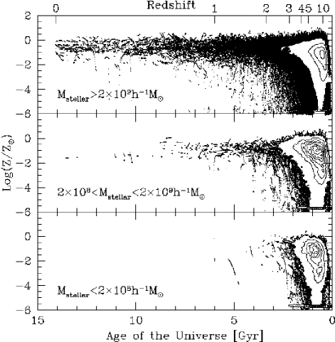
Figure 5.— Metallicity distribution of stars for the same subsamples as in Figure 2. Each point in the figure corresponds to one stellar particle in the simulation with different masses. The abscissa is the age of the universe going from right to left, and the contours are of the number density distribution of stellar particles on an equally spaced logarithmic scale. The mass-weighted mean metallicity at each redshift is given in § 6. Stars formed earlier ($z>4$) have wide range of metallicity ranging from $10^{-6}-1.0Z_{\odot}$, while those formed at $z<1$ have roughly $0.1-1.0Z_{\odot}$.

Let us now consider the G-dwarf problem; the fact that there are too few metal poor stars in the solar neighborhood compared to the closed box model (van den Bergh, 1962; Schmidt, 1963). In our model, a large fraction of stars formed in an early epoch, and such a population contains a significant fraction of metal poor stars. A histogram analysis of the metallicity distribution at $z=0$ shows that 50% of stars have $Z<0.3Z_{\odot}$ in our simulation. This is roughly the same as the prediction of the closed box model, whereas the observation shows the fraction of these stars to be only a few percent (Pagel & Patchett, 1975; Sommer-Larsen, 1991). The qualitative trend of our prediction does not seem to be easily modified. We ascribe, however, the presence of large metal poor stars in our simulation to our inability of resolving the internal structure of galaxies (i.e.disk from bulge). If the disk is a later addition to the bulge as the observations suggest (Fukugita, Hogan, & Peebles, 1996), it would contain little metal poor stars, as is clear from Figure 5 above. The material accreted onto galaxies at low-redshift was already polluted by metals from bulge stars (Ostriker and Thuan, 1975). A high fraction of metal poor stars could occur in the CDM model, when we do not distinguish the disk and the bulge components. This view is consistent with the work by Kauffmann (1996), where she provides a natural explanation to the G-dwarf problem, using a semianalytic model, by pre-enrichment by early outflows from dwarf progenitors.

Finally in Figure 6, we show the mean metallicity of galaxies as a function of their stellar mass in the simulation. The mean metallicity of each galaxy is calculated by taking the mass-weighted average of constituent stellar particles. Solid square points are the median, and the solid bars are the quartiles in each mass bin. Massive galaxies ($M_{\rm stellar}>10^{10}h^{-1}{\,\,M_{\odot}}$) at $z=0$ have mean metallicity of $0.1-1.0Z_{\odot}$, while less massive galaxies have a wide range of mean metallicity ranging from $10^{-4}-1.0Z_{\odot}$. There are a few dwarf galaxies which have even $10^{-6}Z_{\odot}$ outside of the figure. The star formation in less massive galaxies (identified at $z=0$) took place with a wide range of metallicity at high-redshift as we saw in the bottom panel of Figure 5, while larger galaxies at $z=0$ had star formation continuing up to the present epoch with normal metallicity of $0.01-1.0Z_{\odot}$. The two solid lines in the figure are obtained from a fit to the observational data of spiral and irregular galaxies given in Figure 4 of Kobulnicky and Zaritsky (1999). We converted the absolute $B$-magnitude to the stellar mass using the relation $\log M_{\rm stellar}=-0.4M_{B}+(2.75\pm 0.20)$, which the majority of galaxies in our simulation follow before dust extinction (see Paper II), and scaled the metallicity by $\log(Z/Z_{\odot})=12+\log(O/H)-8.89$. A good agreement is seen between the simulated result and the observation in the range of $10^{7}<M_{\rm stellar}<10^{10}h^{-1}\,M_{\odot}$. We remark that Kauffmann (1996) obtains a result similar to ours, which again suggests that the reason we are not seeing a similar cumulative distribution to her result and the solar neighborhood observation is simply because we cannot resolve the bulge and the disk into separate components.

Figure 6.— Average metallicity of galaxies vs. mean stellar mass at $z=0$ in the simulation. Each point represents one galaxy. The median in each mass bin is shown as a solid square, and the solid bars with it are the quartiles. The two solid lines in the figure are obtained from the best-fit to the observational data of spiral and irregular galaxies given in Figure 4 of Kobulnicky and Zaritsky (1999). See text for details. Massive galaxies ($M_{\rm stellar}>10^{10}h^{-1}{\,\,M_{\odot}}$) have normal metallicity of $0.1-1.0Z_{\odot}$, while less massive galaxies take a wide range of values ($10^{-4}-1.0Z_{\odot}$).

7. Conclusions

We have studied predictions of the $\Lambda$CDM universe with regard to the star formation history and the stellar metallicity distribution in galaxies. Our purpose has been to clarify what observations would test the validity of the model of galaxy formation based on $\Lambda$CDM. We have first shown that the global SFR averaged over all galaxies declines with a characteristic time-scale of $\tau\approx 6{\rm\,Gyr}$. About a quarter of stars formed by $z\approx 3.5$ and another quarter by $z\approx 2$. This star formation history is consistent with the empirical Madau plot if modest dust obscuration is assumed.

Our calculation indicates that star formation in $L^{*}$ galaxies continues intermittently to the present epoch as they accrete gas and merge with smaller systems with a decline rate corresponding to an e-folding time of $\tau\approx 6{\rm\,Gyr}$. Star formation in less massive galaxies ceases earlier with an e-folding time of $\tau\lesssim 1{\rm\,Gyr}$. In particular, dwarf galaxies cease their star formation by $z=2$. It is not excluded that minor star formation activity at low-redshift is missed in our calculation due to yet insufficient resolution, but it is unlikely that the global trend would be modified. We consider that this is a feature generic to the CDM structure formation scenario, and observational tests would provide a vital test.

Stars formed in the CDM galaxy formation scenario do not follow a unique age-metallicity relation, but show a considerable spread of metallicity for a given age of stars. Metallicity of very young stars spreads from $0.1-1.0Z_{\odot}$. The spread gradually increases towards high redshift. It takes $0.01-1.0Z_{\odot}$ at $z=2$. At $z=3$, the distribution spreads over from $10^{-6}Z_{\odot}$ to super-metal rich ($3Z_{\odot}$). Young stars are necessarily metal rich, but old stars are not necessarily metal poor. The variation of the mean metallicity with cosmic time is only gradual. The average metallicity for galaxies at $z\approx 1$ differs little from that of local galaxies.

On the other hand, mean metallicity varies as a function of the mass of galaxies. Less massive galaxies are metal poor. Another interesting prediction is that mean metallicity of dwarf galaxies today ranges widely ($10^{-4}-1Z_{\odot}$), which reflects the large scatter of metallicity of stars formed at high-redshift.

The G-dwarf problem in the solar neighborhood offers an interesting insight for formation of galactic structure. If we apply the prediction of the metallicity distribution to solar neighborhood, we encounter the G-dwarf problem: the prediction of the metallicity distribution does not differ much from that of the closed-box model. In our case, however, the G-dwarf problem would be solved if bulges are early entities and disks are later additions.

We have briefly discussed observational tests for each item of the predictions. In many aspects the predictions are supported by observational evidence, but for some aspects the predictions do not seem to agree with the current interpretation of the observations. The currently available observations, however, are sometimes controversial among authors or do not offer unique interpretations free from various working assumptions. We consider that decisive tests will be a task for the future.

References

- Alonso-Herrero et al. (1996) Alonso-Herrero, A., Aragon-Salamanca, A., Zamorano, J., & Rego, M. 1996, MNRAS, 278, 417
- Arnett (1996) Arnett, D., 1996, Supernovae and Nucleosynthesis, Princeton University Press, pp.496
- Balbi et al. (2000) Balbi, A., et al. 2000, ApJ, 545, L1
- Baugh et al. (1998) Baugh, C. M., Cole, S., Frenk. C. S., & Lacey, C. G., 1998 ApJ, 498, 504
- Blumenthal et al. (1984) Blumenthal, G. R., Faber, S. M., Primack, J. R., & Rees, M. J. 1984, Nature, 311, 517
- Bode et al. (2000) Bode, P., Ostriker, J. P., and Turok, N., preprint (astro-ph/0010389)
- Bruzual & Charlot (1993) Bruzual, A. G. & Charlot, S., 1993, ApJ, 405, 538
- Bryan & Norman (1995) Bryan, G. L. & Norman, M. L. 1995, AAS, 187.9504
- Cen and Ostriker (1992a) Cen, R. and Ostriker, J. P. 1992a, ApJ, 393, 22
- Cen and Ostriker (1993) Cen, R. and Ostriker, J. P. 1993, ApJ, 417, 404
- Cen and Ostriker (1999c) Cen, R. and Ostriker, J. P. 1999c, ApJ, 519, L109
- Cen and Ostriker (2000) Cen, R. and Ostriker, J. P. 2000, ApJ, 538, 83
- Cole et al. (2000) Cole, S., Lacey, C. G., Baugh, C. M., & Frenk, C. S. 2000, MNRAS, 319, 168
- Dave, Dubinski, & Hernquist (1997) Dave, R., Dubinski, J., & Hernquist, L. 1997, New Astronomy, 2, 277
- Davis et al. (1985) Davis, M., Efstathiou, G., Frenk, C. S., & White, S. D. M. 1985, ApJ, 292, 371
- Dekel & Silk (1986) Dekel, A. and Silk, J., ApJ, 1986, 303, 39
- Edelson and Malkan (1986) Edelson, R. A. and Malkan, M. A. 1986, ApJ, 308, 59
- Edvardsson et al. (1993) Edvardsson, B., Andersen, J., Gustafsson, B., Lambert, D. L., Nissen, P. E., & Tomkin, J. 1993, A&A, 273, 101
- Efstathiou, Sutherland, & Maddox (1990) Efstathiou, G., Sutherland, W. J., & Maddox, S. J. 1990, Nature, 348, 705
- Efstathiou (1992) Efstathiou, G., 1992, MNRAS, 256, 43
- Eisenstein and Hut (1998) Eisenstein, D. J. and Hut, P. 1998, ApJ, 498, 137
- Fan et al. (2000) Fan, X., et al. 2000, AJ, 120, 1167
- Frogel & Whitford (1987) Frogel, J. A. and Whitford, A. E. 1987, ApJ, 320, 199
- Fukugita, Hogan, and Peebles (1998) Fukugita, M., Hogan, C. J., Peebles, P. J. E., 1998, ApJ, 503, 518
- Fukugita, Hogan, & Peebles (1996) Fukugita, M., Hogan, C. J., Peebles, P. J. E., 1996, Nature, 381, 489
- Gallagher, Hunter, & Tutukov (1984) Gallagher, J. S., Hunter, D. A., Tutukov, A. V. 1984, ApJ, 284, 544
- Gnedin (2000b) Gnedin, N. Y. 2000b, ApJ, 542, 535
- Gnedin (2000a) Gnedin, N. Y. 2000a, ApJ, 535, L75
- Gnedin (1998) Gnedin, N. Y. 1998, ApJ, 294, 407
- Grebel (1997) Grebel, E. K. 1997, Reviews in Modern Astronomy, 10, 29
- Hu, et al. (2000) Hu, W., Fukugita, M., Zaldarriaga, M., & Tegmark, M. 2001, ApJ, 549, 669
- Kauffmann et al. (1999a) Kauffmann, G., Colberg, J. M., Diaferio, A., & White, S. D. M., 1999a, MNRAS, 303, 188
- Kauffmann (1996) Kauffmann, G. 1996, MNRAS, 281, 475
- Katz, Weinberg, & Hernquist (1996) Katz, N., Weinberg, D. H., & Hernquist, L. 1996, ApJS, 105, 19
- Kobulnicky and Zaritsky (1999) Kobulnicky, H. A. and Zaritzky, D. 1999, ApJ, 1999, 511, 118
- Kravtsov, Klypin, & Khokhlov (1997) Kravtsov, A. V., Klypin, A. A., & Khokhlov, A. M. 1997, ApJS, 111, 73
- Lange et al. (2000) Lange, A. E., et al. 2000, preprint (astro-ph/0005004)
- Lanzetta et al. (1999) Lanzetta, K. M., et al. 1999, the proceedings of “The Hy-Redshift Universe: Galaxy Formation and Evolution at High Redshift”, ASP Conference Series, Vol. 193, Ed. A. J. Bunker and W. J. M. van Breugel, p.544
- Majewsky (1993) Majewsky, S. R. 1993, ARA&A, 31, 575
- Mateo (1998) Mateo, M. 1998, ARA&A, 36, 435
- McWilliam & Rich (1994) McWilliam, A. & Rich, R. M. 1994, ApJS, 91, 749
- McWilliam (1997) McWilliam, A. ARA&A, 1997, 35, 503
- Nagamine, Fukugita, Cen, and Ostriker (2001) Nagamine, K., Fukugita, M., Cen, R., & Ostriker, J. P. 2001, preprint (astro-ph/0102180; Paper II)
- Nagamine et al. (2000) Nagamine, K., Cen, R., and Ostriker, J. P. 2000, ApJ, 541, 25
- Navarro & Steinmetz (1997) Navarro, J. F. & Steinmetz, M. 1997, ApJ, 478, 13
- Ostriker and Steinhardt (1995) Ostriker, J. P. and Steinhardt, P. J. 1995, Nature, 377, 600
- Ostriker and Thuan (1975) Ostriker, J. P. and Thuan, T. X. 1975, ApJ, 202, 353
- Pagel & Patchett (1975) Pagel, B. E. J. and Patchett, B. E. 1975, MNRAS, 172, 13
- Pearce et al. (1999) Pearce, F. R., et al. 1999, ApJ, 521, L99
- Pettini et al. (2000) Pettini, M., Steidel, C. C., Adelberger, K. L., Dickinson, M., & Giavalisco, M. 2000, ApJ, 528, 96
- Phillips, Ostriker, & Cen (2000) Phillips, L. A., Ostriker, J. P., & Cen, R. 2000, preprint (astro-ph/0011348)
- Quinn, Katz, & Efstathiou (1996) Quinn, T., Katz, N., & Efstathiou, G. 1996, MNRAS, 278, L49
- Rees (1986) Rees, M. J., MNRAS, 1986, 218, 25
- Rich (1988) Rich, R. M. AJ, 95, 828
- Rocha-Pinto et al. (2000a) Rocha-Pinto, H. J., Maciel, W. J., Scalo, J., & Flynn, C. 2000a, A&A, 358, 850
- Rocha-Pinto et al. (2000b) Rocha-Pinto, H. J., Scalo, J., Maciel, W. J., & Flynn, C. 2000b, A&A, 358, 869
- Ryu et al. (1993) Ryu, D., Ostriker, J. P., Kang, H., and Cen, R. 1993, ApJ, 414, 1
- Sandage (1986) Sandage, A. 1986, A&A, 161, 89
- Scalo (1986) Scalo, J. N., 1986, Fundam. Cosmic. Phys., 11, 1
- Schmidt (1963) Schmidt, M. 1963, ApJ, 137, 758
- Sommer-Larsen (1991) Sommer-Larsen, J. 1991 MNRAS, 249, 368
- Somerville, Primack, & Faber (2001) Somerville, R. S., Primack, J. R., & Faber, S. M. 2001, MNRAS, 320, 504
- Somerville and Primack (1999) Somerville, R. S., and Primack, J. R., 1999, MNRAS, 310, 1087
- Steidel et al. (1999) Steidel, C. C., Adelberger, K. L., Giavalisco, M., Dickinson, M., Pettini, M., 1999, ApJ, 519, 1
- Turner and White (1997) Turner, M. S. and White, M. 1997, Phys. Rev. D, 56, 4439
- van den Bergh (1962) van den Bergh, S. 1962, AJ, 67, 486
- van den Bergh (1998) van den Bergh, S. 1998, A&A review, 9, 273
- Weinberg, Hernquist, & Katz (1997) Weinberg, D. H., Hernquist, L., & Katz, N. 1997, ApJ, 477, 8
- White & Frenk (1991) White, S. D. M. & Frenk, C. S. 1991, ApJ, 379, 52