Apparent and actual galaxy cluster temperatures

Abstract

The redshift evolution of the galaxy cluster temperature function is a powerful probe of cosmology. However, its determination requires the measurement of redshifts for all clusters in a catalogue, which is likely to prove challenging for large catalogues expected from XMM–Newton, which may contain of order 2 000 clusters with measurable temperatures distributed around the sky. In this paper we study the apparent cluster temperature, which can be obtained without cluster redshifts. We show that the apparent temperature function itself is of limited use in constraining cosmology, and so concentrate our focus on studying how apparent temperatures can be combined with other X-ray information to constrain the redshift. We also briefly study the circumstances in which non-thermal spectral features can give redshift information.

1 Introduction

Considerable attention has been devoted to the study of the evolution of the galaxy cluster temperature function with redshift, which promises to be an extremely powerful probe of the density parameter (Frenk et al. 1990; Oukbir & Blanchard 1992; Viana & Liddle 1996; Eke, Cole & Frenk 1996). Even very small numbers of high-mass, high-redshift clusters can rule out the critical-density paradigm; indeed, several authors claim that they have already done so (Henry 1997; Bahcall & Fan 1998; Eke et al. 1998) though this remains controversial (Sadat, Blanchard & Oukbir 1998; Reichart et al. 1999; Viana & Liddle 1999). In order to fully apply this method, the cluster masses must be accurately determined and the usual technique is to use the gas temperature as measured from the X-ray emission. In addition the cluster redshift is required, both to place it correctly in the evolutionary sequence, and because the redshift is needed to convert the apparent temperature into the actual cluster temperature.

For existing catalogues of clusters for which the temperatures could be estimated, obtaining the redshifts proved a manageable task, as the number of clusters with sufficient photon counts to allow temperature determination was small. This is set to change with observations by the XMM–Newton (hereafter just XMM) satellite; in a recent paper (Romer et al. 1999) we showed that a planned serendipitous cluster survey which will analyze all XMM–EPIC frames suitable for serendipitous cluster detection, Xcs, may contain as many as 10 000 galaxy clusters of temperature 2 keV and above, of which around 2 000 may have sufficient photon counts to allow the temperatures to be accurately estimated without further X-ray observations. Given that these will be distributed more or less randomly across the sky, follow-up to obtain spectroscopic redshifts represents a substantial task. The main focus of this paper is on the use of the full available X-ray information to optimize the follow-up efficiency onto the high-redshift population.

Although a survey like the Xcs is likely to contain around two thousand clusters with high enough photon counts to permit an accurate temperature estimate, the thermal bremsstrahlung spectrum only gives the apparent temperature

$$T_{{\rm app}}=\frac{T}{1+z}\,,$$ (1)

with the true temperature not being known until the redshift is determined. For very luminous clusters this degeneracy may be broken by visible spectral lines such as the Iron K line complex at $7$ keV, but this will be challenging for most clusters and we defer discussion of this possibility until the end of the paper.

In this paper we discuss several aspects of apparent temperatures and the estimation of cluster redshifts from X-ray data. Apparent temperatures of clusters were first discussed by Oukbir & Blanchard (1997) in the context of the ROSAT all-sky survey. They also noted the curious point that even in the absence of redshifts the apparent temperature should still be a good estimator of relative cluster masses; for example in a critical-density model scaling laws predict $M\propto T^{3/2}/(1+z)^{3/2}\propto T_{{\rm app}}^{3/2}$.

We focus on issues of apparent temperatures relevant to the XMM satellite. First of all, we analyze whether the apparent temperature function (that is, the number density of clusters observed above a given apparent temperature $T_{{\rm app}}$) might in itself prove a useful probe of cosmology. The answer will be that it proves of limited use, demonstrating the importance of determining cluster redshifts at the earliest possible stage. In that light, we go on to consider how other X-ray observables can be combined with the apparent temperatures in order to constrain the redshifts, particularly with a view to eliminating low-redshift clusters from the follow-up candidate list. The main observables are the angular size and the apparent luminosity of the clusters, and it is the latter which proves powerful in combination with the apparent temperature. We also briefly study xspec spectral simulations to assess the likelihood of redshift determination from X-ray spectral lines.

2 The apparent temperature function

Before considering redshift estimation, it is worth exploring whether the X-ray apparent temperature function $N(>T_{{\rm app}})$ might yield useful constraints on cosmology. Unlike the real temperature function $N(>T,z)$, which can also be taken as a function of redshift, the apparent temperature function includes clusters from all redshifts. The main application of the cluster number density is to limit the matter density in the Universe, and so we focus on that.

Figure 1: The number of clusters with apparent temperature above a given value, plotted for three different cosmologies. The numbers assume a survey area of 800 square degrees, and assume a catalogue with observed flux limit $10^{-13}\,{\rm erg}\,{\rm s}^{-1}\,{\rm cm}^{-2}$.

We compute the apparent temperature function using the Press–Schechter techniques of Viana & Liddle (1999), to which we refer the reader for details. The key assumptions of the method are that the temperature can be obtained from the mass via the usual scaling relations (normalized to hydrodynamical cluster simulations), and that the relationship between luminosity and temperature observed in the present Universe (Allen & Fabian 1998) is valid also at high redshift. This latter assumption is quite likely to prove incorrect at some level and is subject to modification when improved observations become available. We study the same three cold dark matter (CDM) cosmologies as in Viana & Liddle (1999). One is a critical-density cosmology, and the other two are low-density models with $\Omega_{0}=0.3$, one of which is an open model and the other the currently-favoured spatially-flat model with a cosmological constant. In each case the models are normalized to give a good fit to the present-day cluster number density (Viana & Liddle 1996, 1999) by adjusting the dispersion $\sigma_{8}$ of the power spectrum.

Figure 2: The apparent temperature function for critical-density models with different $\sigma_{8}$ as shown. The curve $\sigma_{8}=0.56$ is the standard cluster normalization used in Figure 1.

Figure 1 shows the apparent temperature function predicted, assuming a survey with a flux limit of $10^{-13}\,{\rm erg}\,{\rm s}^{-1}\,{\rm cm}^{-2}$ in the [0.5, 2] keV band, which is around the mean level at which XMM would expect to have sufficient photons for temperature estimation in a typical pointing. The curves look quite promising, with a factor of a few difference between the low-density and critical-density cases. Unfortunately though, this does not take into account the effect of varying other parameters, and it transpires that there is a strong degeneracy with the normalization $\sigma_{8}$ of the matter power spectrum. Figure 2 shows the predictions for a series of critical-density models with different values of $\sigma_{8}$, and shows a strong dependence which is capable of swamping the dependence on $\Omega_{0}$. Taking for example the flat case, the normalization of the power spectrum we use takes $\sigma_{8}\Omega_{0}^{-0.47}=0.56$ (Viana & Liddle 1999), with an uncertainty of about 20 per cent at the 95% confidence level, so all the curves shown in Figure 2 are plausible. From the curves, we estimate that the number of clusters above a given apparent temperature scales roughly as

$$N\propto\left(\sigma_{8}\Omega_{0}^{-0.47}\right)^{8}\,\frac{1}{\Omega_{0}}\,,$$ (2)

so the first dependence dominates the latter. This is the familiar degeneracy of the low-redshift cluster sample, arising because at any given apparent temperature the sample is dominated by nearby clusters. The apparent temperature function can therefore be used to measure that combination to high accuracy, but nothing else.

Although the previous figures illustrate the expected behaviour, the assumption of a fixed flux cut is over-simplistic for XMM. In reality, whether or not a cluster has a measurable temperature depends on the cluster temperatures and redshifts themselves, and also on the distribution of pointing durations. In Romer et al. (1999) we established a large set of simulations allowing us to determine which clusters can be identified in XMM frames, and the subset of these for which temperature estimation is available. Of course, given those data a fixed flux cut-off can be imposed to give a flux-limited sample, but we can also simulate the complete expected data-set. We have done so, and we have found it makes negligible difference to the predicted curves.

Figure 3: The predicted angular extent as a function of redshift for a clusters of apparent temperatures 2 keV (top) and 4 keV (bottom).

3 Redshift estimates from X-ray observables

In order to fully capitalize on a large X-ray cluster catalogue, redshifts are clearly essential for those clusters with measured apparent temperatures. In cosmology, this allows the evolution of the temperature function to be used to break the low-redshift degeneracy. Given the expected size of the data set, full spectroscopic follow-up is a substantial task, and in this section we consider ways in which other X-ray observables can be used along with the apparent temperatures to help optimize the follow-up strategy by providing estimated cluster redshifts.

Figure 4: The predicted observed flux as a function of redshift for a clusters of apparent temperatures 2 keV (top) and 4 keV (bottom). We have followed the convention of giving the flux in the ROSAT band, though the band is irrelevant as clusters of the same apparent temperature share the same spectral shape.

3.1 X-ray flux and angular extent

In addition to the spectrum of the photons received, the main X-ray observables are the angular extent of the clusters and the observed flux. In Figures 3 and 4 we plot the expected redshift dependence of these, for the three cosmologies we are considering, and for clusters of apparent temperature 2 keV and 4 keV. Note that these plots differ from more standard ones in that it is the apparent temperature which is fixed, so that as the cluster is moved to higher redshift its temperature increases. The quantity $r_{50}$ is the radius of the region enclosing the inner 50 per cent of the total cluster flux, which for a cluster with an isothermal $\beta$-profile and $\beta=2/3$ is a factor of $\sqrt{3}$ larger than the cluster core radius, $r_{{\rm c}}$. Unfortunately, at present the mechanism that gives rise to the cluster core radius is not well understood, and hence neither is how $r_{{\rm c}}$ is related to X-ray temperature or luminosity nor how it may change with redshift. Therefore we simply take the empirical relation between $r_{{\rm c}}$ and X-ray luminosity given in Jones et al. (1998) and assume it does not evolve with redshift. Luminosity, also, cannot yet be predicted from first principles, and so we assume that the observed low-redshift relation between temperature and luminosity does not evolve with redshift. Once XMM has observations to high redshift, any evolution is readily incorporated.

These plots confirm the standard beliefs, based on consideration of clusters of fixed properties viewed at different redshifts, that the apparent size is only a weak function of redshift beyond 0.3 or so, while the flux continues to evolve significantly. The former is therefore not useful as a redshift discriminator, even though XMM should resolve all clusters, while the latter is. We checked whether the situation would change if the core radius evolved in a self-similar way, maintaining a fixed size relative to the virial radius, but though in this case the apparent size does depend more on redshift, it still does not change as strongly as the flux.

In order to ascertain how useful the flux is as a redshift estimator, and to get a feeling for the importance of scatter in the luminosity–temperature relation and uncertainties in the measured temperatures, we have carried out Monte Carlo simulations of catalogues corresponding to three years of Xcs data. We assume a flat, cosmological constant dominated, Universe with $\Omega_{0}=0.3$. A realistic simulation needs to include both intrinsic scatter in the luminosity at a given temperature, and the errors in temperature measurement. The intrinsic scatter in the luminosity distribution is estimated from hydrodynamical simulations as being 20 per cent at one-sigma (O. Muanwong, private communication).

Figure 5: Fitted apparent temperature versus input apparent temperature for simulated XMM cluster spectra after the subtraction of 100 (upper panel) and 1000 (lower panel) background counts. All input spectra were created using fakeit in xspec and contained 1000 net cluster counts. The dotted lines delineate input apparent temperature plus and minus 20 per cent.

We estimated the likely temperature errors using xspec simulations. In Figure 5, it can be seen that, for a wide range of input apparent temperatures, the mean fitted apparent temperature is roughly equal to the input and that the 1 sigma errors bars fall within 20 per cent of the mean. The xspec-based methodology used to produce this figure (i.e. production of simulated spectra from cluster and background spectral models, background subtraction, spectral fitting etc.) was similar to that used in Romer et al. (1999) (e.g. see Figure 4 and §5.2 of that paper) to estimate the errors on temperature fits for clusters with known redshifts. The only notable modification to that methodology was the fixing of the redshift in the fits at $z=0$ rather than at the redshift of the input spectrum. As in Romer et al. (1999), 20 fake spectra per parameter combination were created and then fitted in order to derive a stable mean and a realistic error distribution. Figure 5 shows 84 parameter combinations; six temperatures (2, 4, 6, 8, 10 and 12 keV), seven redshifts ($z=$ 0.05, 0.1, 0.2, 0.4, 0.6, 0.8, 1.0) and two background contaminations (100 and 1000 background counts for the upper and lower plots respectively). The net number of cluster counts after background subtraction was fixed at 1000; this was the threshold adopted in Romer et al. (1999) to predict the number of Xcs clusters that will yield temperature estimates. For the purposes of illustration we have shown two extremes of the expected background contamination; most spectra will be contaminated by a few hundred background counts (with an imposed upper limit of 1000, see §5.2 of Romer et al. (1999)). For typical clusters the true errors are likely to be less than 20 per cent, because the number of cluster counts will be greater, but this assumption may be more realistic for the distant, fainter clusters in which we are primarily interested. Unfortunately at present computational limitations prevent us from carrying out fully self-consistent simulations where the expected cluster counts are derived from the modelled cluster properties, and the XMM in-flight background estimates are not yet available.

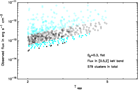
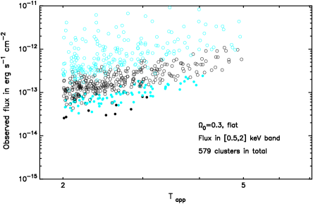
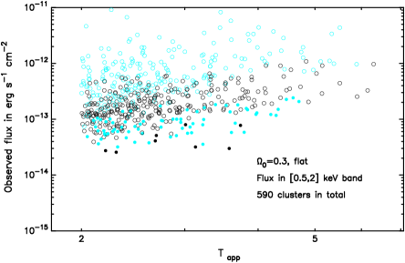
Figure 6: The expected location of clusters in the X-ray flux versus apparent temperature plane. The clusters are divided into four redshift intervals: $0<z<0.3$, cyan/grey open circles; $0.3<z<0.6$, black open circles; $0.6<z<0.9$, cyan/grey points; $z>0.9$, black points. These simulations are for a flat low-density Universe, for three years of Xcs data. The upper panel assumes no error in the apparent temperatures, and no scatter in the luminosity–temperature relation. The middle panel introduces scatter in the luminosity (at fixed temperature), while the bottom panel is the realistic situation of both luminosity scatter and temperature measurement errors.

The results of the Monte Carlos are shown in Figure 6, in which the different colours/symbols show different bins in redshift. For reference, the upper panel shows the location of clusters assuming the apparent temperatures are measured precisely, and that there is no scatter in the luminosity at a given temperature or errors in the temperature measurements. The middle panel show the effect of including luminosity scatter alone, which is not particularly significant, on the same Monte Carlo realization. The effect of adding temperature uncertainties (in addition to luminosity scatter) is shown in the bottom panel of Figure 6. The plot shows only those clusters whose measured apparent temperature exceeds 2 keV, regardless of what their true apparent temperature is. One could attempt to reduce the temperature errors by making extra pointed observations once the clusters have been identified serendipitously, but the high-redshift ones are typically only appearing in the longest serendipitous exposures anyway.

A feature of the bottom panel is that it contains more clusters than the upper two panels. This is because while temperature errors in an individual cluster are as likely to be overestimates as underestimates, there are more low temperature clusters to ‘scatter up’ than high temperature ones to scatter down. Careful Monte Carlo simulations are necessary to take out this bias (see e.g. Viana & Liddle 1999) when estimating the true temperature functions.

Returning to our motivation in making these plots, the aim was to test whether the scattering of the points significantly decreases the ability to identify the high-redshift cluster population within Xcs using observed X-ray flux and apparent temperature. From Figure 6, we see that the segregation of clusters with redshift remains quite good. For example, drawing a line between the points $(2,10^{-13})$ and $(7,10^{-12})$ clearly differentiates between local clusters, with $z<0.3$, which lie above the line, and clusters with $z>0.6$ which lie below the line; it reduces the sample to 44% of its original size without losing any of the $z>0.6$ clusters. A more stringent cut a factor of two lower in flux can create a sample of mostly high-redshift clusters; it reduces the sample to 117 clusters, including 65 of the 78 clusters above $z=0.6$.

We conclude that the combination of apparent temperature and X-ray flux can be used as a redshift indicator. Analysis of the Monte Carlo data shows that some care will be needed; the general tendency of the temperature errors to scatter clusters upwards in temperature usually results in an overestimation of the redshift, though this can readily be accounted for. Taking scatter in luminosity and temperature into account, we find that an estimated redshift with 33 per cent $1$-sigma uncertainty at high redshift should be readily achievable, though the absolute scale relating flux and apparent temperature to redshift will require calibration against real data. Most likely we have been quite conservative in the assessment of temperature errors, so the actual accuracy of the estimation may considerably exceed this in practice.

We should stress that Figure 6 is based on several assumptions, such as non-evolution of the luminosity–temperature relation with redshift, which are at best weakly tested by current observations. However, improved information from early XMM and Chandra observations can readily be incorporated when available to improve the use of flux and apparent temperature as a redshift estimator.

A possible danger in using the flux is contamination of the cluster counts by point sources, for example AGN within cluster galaxies. For the ROSAT satellite, with its low spatial resolution, this has proved a problem for several clusters, especially those at high redshift; see for example Romer et al. (2000) and §6.2.2 of Romer et al. (1999). The problem will be considerably less significant for XMM given its much higher spatial resolution.

3.2 X-ray spectral features

For suitably luminous clusters one may see emission lines in the spectrum which allows the degeneracy between $T$ and $z$ to be broken using the serendipitous X-ray data alone. The existence of such lines is illustrated in Figure 7, where we show model spectra for three clusters, chosen to have the same apparent temperature of $2$ keV and placed at redshifts $z=0$, $0.5$ and $1$. The spectra were generated using the xspec fakeit routine from absorbed Raymond–Smith (1977) plasma models assuming a neutral hydrogen column density of $4\times 10^{20}$ atoms/cm² and a metal abundance of 0.3 times the solar value. The spectra have been folded through the XMM EPIC-pn response files epn_new_rmf.fits and epn_thin_arf.fits, available from astro.estec.esa.nl. For the purposes of this illustration, the exposure times were chosen so that each spectrum contained one million counts in the $0.5$–$10$ keV band when the metal abundance was zero, which is vastly higher than that expected for real clusters.

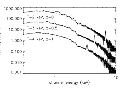
Figure 7: Simulated spectra for clusters with apparent temperature $2$ keV, assuming an unrealistically large flux of a million counts for each cluster. The dashed lines show the zero metal abundance curves; variations from these curves are due to the effects of line emission. To allow easier comparison, the $T=3$ keV and $T=4$ keV spectra have been divided by 10 and 100 respectively before plotting.

In addition to the thermal bremsstrahlung continuum (the grey lines), several features due to line emission are visible, for example the Iron K line complex at 7 KeV and the rich collection of emission lines in the energy range 0.6 keV to 2 keV, most notably the complex of iron, neon and magnesium lines at $\simeq 1$ keV. As Figure 7 shows, the 7 keV (rest frame) Iron line complex moves to lower energies as redshift increases. A disadvantage of the Iron line complex is that it falls at an energy at which both the cluster spectrum and energy response of XMM has fallen off significantly. In principle, one could use the line complex at $\simeq 1$ keV, where XMM is significantly more sensitive, though in practice this might only be possible for the low-temperature systems as the contrast of the line emission against the thermal continuum drops off rapidly with increasing temperature (see Figure 7).

Unfortunately, for the purposes of the Xcs, the illustrative Figure 7 is unrealistic because it contains far too many counts and ignores the effect of the cosmic and particle backgrounds. Our guideline threshold for Xcs clusters to have measurable temperatures is one thousand counts, and as seen from Figure 6 the brightest clusters (which are of course the nearby ones) will have up to around one hundred thousand counts (clusters of the same apparent temperature share the same spectral shape and so the count rate is proportional to the flux). In Figure 8 we show a more realistic, though still optimistic, simulation of a $z=1$, $T=4$ keV model spectrum containing ten thousand counts in the $0.5$–$10$ keV range, again ignoring the effects of background contamination. For spectra of this quality, or worse, one would need to use template fitting, rather than eyeballing, to derive redshift estimates. We conclude that X-ray lines may well allow accurate redshift estimation for many low-redshift clusters, but is unlikely to work well for high-redshift ones. Estimating the limiting redshift will require more detailed information on the backgrounds than is presently available.

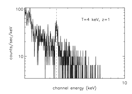
Figure 8: Part of a cluster spectrum which contains ten thousand counts in the 0.5-10 keV band. This spectrum was derived from the same model that produced the highest redshift of the three spectra presented in Figure 7. The dotted grey line marks the expected position of the redshifted Iron K line complex.

We note that few, if any, X-ray redshifts will be derived from the XMM RGS cameras, despite them having much higher spectral resolution than the EPIC cameras. This is because the RGS disperses energy from sources across the field of view, so it would be extremely difficult to isolate the spectrum from an Xcs cluster (an extended off-axis source) from that of the pointing target. For an example of how RGS can be used to study nearby bright cluster targets, see Tamura et al. (2000).

4 Conclusions

In this paper we have studied various aspects of apparent cluster temperatures relevant to XMM observations. The apparent temperature function will be readily derived from XMM data, but will primarily be useful in constraining the degenerate combination familiar from low-redshift cluster number density studies, $\sigma_{8}\Omega_{0}^{-\alpha}$ with $\alpha\sim 0.5$, and is unlikely to usefully probe the density parameter itself.

To fully exploit a galaxy cluster catalogue, cluster redshifts are essential, and we have studied how other X-ray properties can be combined with the apparent temperature to select follow-up candidates efficiently. Assuming point source contamination can be recognized from the high-resolution imaging, it appears that the cluster flux, when combined with the apparent temperature, will yield a good indication of the cluster redshift, especially once early XMM observations have been used to calibrate the relation.

Finally, we remark that further useful information towards estimating the redshifts may come from imaging data in the optical and infra-red once cluster candidates have been identified in the X-ray. A good example is the K band luminosity of the brightest cluster galaxy, which exhibits a tight correlation with redshift for X-ray luminous clusters, as shown by Collins & Mann (1998) and Burke, Collins & Mann (2000). In many cases it may also be possible to carry out photometric redshifting of cluster galaxies, for example using Sloan Digital Sky Survey and VISTA data.

References

- [Allen & Fabian 1998] Allen S. W., Fabian A. C., 1998, MNRAS, 297, L57
- [Bahcall & Fan 1998] Bahcall N.A., Fan X., 1998, ApJ, 504, 1
- [Burke et al. 2000] Burke D. J., Collins C. A., Mann R. G., 2000, ApJ, 532, L105
- [Collins & Mann 1998] Collins C. A., Mann R. G., 1998, MNRAS, 297, 128
- [Eke et al. 1996] Eke V. R., Cole S., Frenk C. S., 1996, MNRAS, 282, 263
- [Eke et al. 1998] Eke V. R., Cole S., Frenk C. S., Henry P., 1998, MNRAS, 298, 1145
- [Frenk et al. 1990] Frenk C. S., White S. D. M., Efstathiou G., Davis M., 1990, ApJ, 351, 10
- [Henry 1997] Henry J. P., 1997, ApJ, 489, L1
- [Jones et al 1998] Jones L. R., Scharf C., Ebeling H., Perlman E., Wegner G., Malkan M., Horner D., 1998, ApJ, 495, 100
- [Mohr et al. 2000] Mohr J. J., Reese E. K., Ellingson E., Lewis A. D., Evrard A. E., 2000, ApJ, 544, 109
- [Oukbir & Blanchard 1992] Oukbir J., Blanchard A., 1992, A&A, 262, L21
- [Oukbir & Blanchard 1997] Oukbir J., Blanchard A., 1997, A&A, 317, 1
- [Pierpaoli et al. 2000] Pierpaoli E., Scott D., White M., 2000, astro-ph/0010039
- [Raymond & Smith 1977] Raymond J.C., Smith B.W. 1977, ApJSupp, 35, 419
- [Reichart et al. 1999] Reichart D.E., Nichol R.C., Castander F.J., Burke D.J., Romer A.K., Holden B.P., Collins C.A., Ulmer M.P., 1999, ApJ, 518, 521
- [Romer et al. 2001] Romer A. K., Viana P. T. P., Liddle A. R., Mann R. G., 2001, ApJ, 547, 594
- [Romer et al. 2000] Romer A. K., et al., 2000, ApJS, 126, 209
- [Sadat et al. 1998] Sadat R., Blanchard A., Oukbir J., 1998, A&A, 329, 21
- [Tamura et al. 2000] Tamura T., et al., 2000, astro-ph/0010362
- [Verde et al. 2000] Verde L., Kamionkowski M, Mohr J. J., Benson A. J., 2000, astro-ph/0007426
- [Viana & Liddle 1996] Viana P. T. P., Liddle A. R., 1996, MNRAS, 281, 323
- [Viana & Liddle 1999] Viana P. T. P., Liddle A. R., 1999, MNRAS, 303, 535