Studying the Galactic Bulge Through Spectroscopy of Microlensed Sources: I. Theoretical Considerations

Abstract

The observed spectra of the microlensed sources towards the Galactic bulge may be used as a tool for studying the kinematics and extinction effects in the Galactic bulge. In this paper, we first investigate the expected distribution of the microlensed sources as a function of depth within the Galactic bulge. Our analysis takes a magnitude limited microlensing survey into account, and includes the effects of extinction. We show that, in the current magnitude limited surveys, the probability that the source lies at the far side of the bulge is larger than the probability that the source lies at the near side. We then investigate the effects of extinction on the observed spectra of microlensed sources. Kurucz model spectra and the observed extinctions towards the Galactic bulge have been used to demonstrate that the microlensed sources should clearly show the effects of extinction which, in turn, can be used as a statistical measure of the contribution of the disk lenses and bulge lenses at different depths. The spectra of the microlensed sources provide a unique probe to derive the radial velocities of a sample which lies preferentially at the far side of the Galactic bulge. The radial velocities, coupled with the microlensing time scales, can thus be useful in studying the 3-dimensional kinematics of the Galactic bulge.

1 INTRODUCTION

The topic of gravitational microlensing has experienced a dramatic increase in scientific interest over recent years. This has been largely due to the realization of its wide-ranging applications, such as the detection of planets and the study of Galactic structure. More than 400 microlensing events have now been detected toward the Galactic bulge and Magellanic Clouds by the microlensing survey teams EROS, MACHO, OGLE, DUO, and MOA. The contribution of the bulge stars to the observed microlensing optical depth towards the Galactic bulge was estimated to be approximately 60%, the other 40% being due to the stars in the Galactic disk (Kiraga & Paczyński, 1994). The optical depth to gravitational microlensing, as estimated from the observed microlensing events by OGLE (Udalski et al., 1994), MACHO (Alcock et al., 1997), EROS Afonso et al. (2003), and MOA Sumi et al. (2003), is significantly larger than the values predicted by theoretical models (Paczyński, 1991). It has been argued (Paczyński et al., 1994) that the observed optical depth can be best explained if the effect of the Galactic bar and its inclination are correctly taken into account. A consequence of the fact that a large fraction of the events are due to bulge-bulge lensing is, as we will show in more detail later, that the lensed stars will preferentially be located on the far side of the bulge in order that there be sufficient stars along the line of sight to cause microlensing. It was suggested by Stanek (1995) that this would mean that there should be a systematic offset in the apparent magnitude between observed stars and lensed stars. We present a similar discussion by examining the model spectra of different spectral classes and investigating the effects of extinction on stars located on the far side of the bulge.

We first calculate the contributions of the different layers in the bulge to the microlensing optical depth, as has previously been calculated by Kiraga & Paczyński (1994) and Zhao, Spergel, & Rich (1995). We have, however, considered the additional effect of extinction in some detail. We then proceed with a discussion on how the spectra of the microlensed sources can be used as a measure of the extinction which, in turn, can be used as a statistical measure of the contribution of the disk lenses and bulge lenses at different depths. We show that the spectra of the microlensed sources can be a useful probe for the 3-dimensional structure of the Galactic bulge. We have also undertaken such a spectroscopic study of the microlensed sources, the details of which are the subject of another paper (Kane & Sahu, 2003).

2 CALCULATING THE PROBABILITY OF MICROLENSING

The aim here is to calculate the microlensing probability for sources at various depths within the Galactic bulge and to see how the microlensing optical depth varies for sources at various depths taking the effect of extinction into account. We first develop the theory for a general distribution of microlensing sources and will later restrict the source distribution to those located in the Galactic bulge. For these calculations, the formalism used by Sahu (Sahu, 1994a, b) shall be adopted.

Firstly, the number of sources observed at various depths shall be estimated. As we will discuss in more detail later, the intrinsic distribution of the Galactic bulge sources can be expressed by an exponential distribution, the density being maximum at the central part and falling on either side. The extinction and the distance modulus increase as one goes deeper into the bulge, and both these effects make the sources fainter. So, in a magnitude limited survey (such as the current ones), the combined effect of the extinction and the distance is a monotonous decrease in the observed number of stars as we go from the nearest to the farthest region along a given line of sight, which needs to be folded in with the intrinsic distribution of the sources in order to obtain their observed distribution.

To express the above effects, let us assume that the ratio of the stellar number density at the central part of the bulge to the stellar density in the near-side of the bulge is $a_{1}$ and the ratio of the stellar number density at the central part of the bulge to the stellar density in the far-side of the bulge is $a_{2}$. Thus, $a_{1}$ and $a_{2}$ include the effects of localized extinctions and the intrinsic distributions.

Let $N_{tot}$ be the number of stars being monitored in a region. Assuming the extinction to be uniform in depth within the bulge, the number of observed stars at any layer $dx$, at a depth of $x$ (as measured from the central plane of the Galactic bulge, see Figure 1), may be expressed as

$$N_{obs}(x)=\left\{\begin{array}[]{ll}N_{0}a_{1}^{-x/d}&\mbox{if $D_{s}<R_{0}$}\\ N_{0}a_{2}^{-x/d}&\mbox{if $D_{s}>R_{0}$}\end{array}\right.$$ (1)

where $N_{0}$ is a constant and represents the observed number of stars per unit depth in the central region of the Galactic bulge and $d$ is the depth to which the bulge extends on either side from the center. $R_{0}$ is the distance to the central region of the bulge and $D_{s}$ is the distance to the source (i.e., the distance from the observer to the plane corresponding to $x$ so that $x={\left|D_{s}-R_{0}\right|}$).

Integrating this expression along the line of sight, we can write

$$N_{tot} = \int_{0}^{d}N_{0}a_{1}^{-x/d}\,dx+\int_{0}^{d}N_{0}a_{2}^{-x/d}\,dx$$ (2)

$$= N_{0}\left[\frac{d}{\ln a_{1}}\left(1-\frac{1}{a_{1}}\right)+\frac{d}{\ln a_{2}}\left(1-\frac{1}{a_{2}}\right)\right]$$

The fraction of area covered by the Einstein rings of all the individual stars lying in front of a source at distance $D_{s}$ may be expressed as

$$A_{f}(D_{s})=\int_{0}^{D_{s}}\pi R_{E}^{2}(D_{d})n(D_{d})\,dD_{d}$$ (3)

where $D_{d}$ is the distance to the lens and $n(D_{d})$ is the stellar number density at distance $D_{d}$. If we define $\rho(D_{d})$ as the average mass density at depth $D_{d}$ then we see that $n(D_{d})=\rho(D_{d})/M$. Since the Einstein ring radius for a lens of mass $M$ in this case is given by

$$R_{E}=\sqrt{\frac{4GM}{c^{2}}\frac{D_{d}(D_{s}-D_{d})}{D_{s}}}$$ (4)

Equation (3) can be rewritten as

$$A_{f}(D_{s})=\frac{4\pi G}{c^{2}}\int_{0}^{D_{s}}\rho(D_{d})\frac{D_{d}(D_{s}-D_{d})}{D_{s}}\,dD_{d}$$ (5)

The instantaneous probability that an observed microlensed star is at a given distance $D_{s}$, can be written as

$$p=\frac{A_{f}(D_{s})N_{obs}(D_{s})}{N_{tot}}$$ (6)

Note that, in our desire to treat both the source and lens distributions in a similar manner, we have chosen our expression for the number of observed stars at $D_{s}$ to be $N_{obs}(D_{s})\,dD_{s}$, and not $N_{obs}(D_{s})\,dD_{s}\,d\Omega$. This would suggest that $N_{obs}(D_{s})$ may increase with $D_{s}$ since the solid angle $d\Omega\propto D_{s}^{2}$. On the other hand, in a magnitude-limited sample, the $N_{obs}(D_{s})$ would decrease with $D_{s}$ since the observed flux decreases as $D_{s}^{-2}$. The above two effects tend to cancel each other, but not exactly, particularly when there is extinction. In our general case of the exponential distribution for the bulge (section 2.3), we have chosen $a_{1}$ and $a_{2}$ to be different, which should absorb this extra effect.

The total microlensing optical depth $\tau$ can now be calculated. If $N_{tot}$ stars within the bulge are being monitored, then the instantaneous probability of observing a lensing event with an amplification of $A>1.34$ is given by

$$P=\int_{b_{n}}^{b_{f}}N_{obs}(D_{s})A_{f}(D_{s})\,dD_{s}$$ (7)

where we assume all the monitored sources to be within the Galactic bulge and, for convenience, we have defined $b_{n}=R_{0}-d$ and $b_{f}=R_{0}+d$ (i.e., the distances from the observer to the near side and far side of the bulge respectively).

The optical depth for microlensing, which is the instantaneous probability that a given star is microlensed, can be written as

$$\tau=P/N_{tot}$$ (8)

Assuming a uniform extinction with depth is a simple model with some inherent uncertainties and is unlikely to be representative of the real extinction in the line of sight to microlensed sources. However, this does not affect the conclusions of this analysis. A full modeling of the extinction has its own uncertainties and is beyond the scope of this work.

It should be noted that in our calculations we are not comparing extinctions at different parts in the bulge but rather we are comparing the differential extinctions between microlensed and non-microlensed sources in the same part of the sky. It is know that the dust layer when looking towards the bulge is patchy and predominantly in the disk (Arp, 1965). However, this will not significantly affect our calculations as the angular distance between the microlensed source and the corresponding lens will be small enough such that the foreground extinction may be considered to be the same for both objects (Zhao, 2000).

We will carry out these calculations using 3 different approximations: (i) constant density of stars between the observer and the source, (ii) constant (but different) densities for the disk and the bulge, and (iii) an exponential density model for the bulge. The last approximation is likely to be the best model, and hence the results of this model will be used in our forthcoming spectral analysis (Kane & Sahu, 2003). For completeness however, we present the calculations in the other two approximations, since these calculations may be useful for other lines of sight, including the lines of sight far from the Galactic Center, and possibly towards the LMC and M31.

2.1 Constant Density Between Observer and Source

First, let us assume a constant density of matter for the lenses between the observer and the source and make the substitution $y=D_{d}/D_{s}$, then equation (5) becomes

$$A_{f}(D_{s}) = \frac{4\pi GD_{s}^{2}}{c^{2}}\int_{0}^{1}\rho(D_{d})y(1-y)\,dy$$ (9)

$$= \frac{2\pi G\rho D_{s}^{2}}{3c^{2}}$$

Since the matter density in the line of sight is constant, extinction is the only effect which changes the observed number density of sources in the line of sight. Let us define the intrinsic stellar density $N_{n}=N_{0}a$ where $N_{0}$ is the observed stellar density at the mid-plane along the line of sight. Let $d_{c}=2d$ be the total depth, and $a_{c}=a^{2}$ which corresponds to the ratio of the stellar density from the near to the far side. In this case, equation (1) takes the form

$$N_{obs}(D_{s})=N_{n}a_{c}^{-D_{s}/d_{c}}$$ (10)

Integrating this expression yields

$$N_{tot}=\int_{0}^{d_{c}}N_{n}a_{c}^{-D_{s}/d_{c}}\,dD_{s}=N_{n}d_{c}\left(\frac{1-1/a_{c}}{\ln a_{c}}\right)$$ (11)

Substituting equations (9-11) into equation (6) yields

$$p=\frac{2\pi G\rho D_{s}^{2}}{3c^{2}d_{c}}\left(\frac{\ln a_{c}}{1-1/a_{c}}\right)a_{c}^{-D_{s}/d_{c}}$$ (12)

This probability $p$ is plotted in Figure 2 as a function of $D_{s}$ assuming a density of $\rho=0.20\,M_{\odot}\mathrm{pc}^{-3}$.

As seen in Figure 2, for $a_{c}=1$ (which corresponds to no extinction), the probability that a given observed microlensed source is at a distance $D_{s}$ increases monotonically with $D_{s}$. It is clear that $A_{f}(D_{s})$, the fractional area covered by the lenses for a source at distance $D_{s}$, increases monotonically with distance. However, for $a_{c}>1$, the number of observed stars decreases with distance because of extinction. As seen in equation (6), $p$ is a multiplication of these two quantities which, as demonstrated in Figure 2, increases steeply with distance for $a_{c}=1$, and increases less steeply with distance for increasing values of $a_{c}$. This is also demonstrated in Table 1 which gives the probabilities that a given microlensed star is at distances $D_{s}=7.0\,\mathrm{kpc}$, $D_{s}=8.0\,\mathrm{kpc}$, and $D_{s}=9.0\,\mathrm{kpc}$ for various values of $a_{c}$. It is worth reiterating here that $p=[A_{f}(D_{s})N_{0bs}(D_{s})/N_{tot}]$ is the probability that a given observed microlensed source is at a distance $D_{s}$, which is distinct from the probability that a given observed star at the distance $D_{s}$ is microlensed; the latter simply scales as the microlensing optical depth $\tau$ which monotonically increases with the distance.

Substituting equation (9) and equation (11) into equation (7) gives

$$P=\frac{2\pi G\rho}{3c^{2}}\frac{N_{tot}}{d_{c}}\left(\frac{\ln a_{c}}{1-1/a_{c}}\right)\int_{0}^{d_{c}}a_{c}^{-D_{s}/d_{c}}D_{s}^{2}\,dD_{s}$$ (13)

where the integrand can be solved analytically via repeated integration by parts. Dividing the result by $N_{tot}$ yields an expression for the optical depth for gravitational microlensing

$$\tau=\frac{2\pi G\rho d_{c}^{2}}{3c^{2}}\frac{a_{c}}{a_{c}-1}\left(\frac{2}{(\ln a_{c})^{2}}-\frac{1}{a_{c}}-\frac{2}{a_{c}\ln a_{c}}-\frac{2}{a_{c}(\ln a_{c})^{2}}\right)$$ (14)

The value of $\tau$ as given in equation (14) is plotted in Figure 3 as a function of $a_{c}$, which shows the variation of optical depth with increasing extinction. As seen from this figure, the optical depth in this case is close to $5\times 10^{-7}$ for a large range of $a_{c}$ since the intrinsic matter distribution, which plays the major role in the determination of optical depth, is constant.

However, the assumption of constant density along the line of sight may be valid for microlensed sources in the Galactic disk (e.g., OGLE-1999-CAR-01 (Udalski et al., 2000)), but can not be applied to sources in the Galactic bulge.

2.2 Constant Density for Disk and Bulge

If we assume a constant density of matter for the lenses in the disk and the bulge, given by $\rho_{d}$ and $\rho_{b}$, respectively, equation (5) becomes

$$A_{f}(D_{s})=\frac{4\pi G}{c^{2}}\left(\int_{0}^{b_{n}}\rho_{d}\frac{D_{d}(D_{s}-D_{d})}{D_{s}}\,dD_{d}+\int_{b_{n}}^{D_{s}}\rho_{b}\frac{D_{d}(D_{s}-D_{d})}{D_{s}}\,dD_{d}\right)$$ (15)

Since the optical depth of microlensing of disk stars is relatively small (Kiraga & Paczyński, 1994), we have assumed that all the sources are within the Galactic bulge, i.e., $b_{n}<D_{s}<b_{f}$.

Making the substitution $y=D_{d}/D_{s}$, equation (15) simplifies to

$$A_{f}(D_{s})=\frac{4\pi GD_{s}^{2}}{c^{2}}\left(\rho_{d}\int_{0}^{b_{n}/D_{s}}y(1-y)\,dy+\rho_{b}\int_{b_{n}/D_{s}}^{1}y(1-y)\,dy\right)$$ (16)

Solving this yields the following expression for the fractional area covered by the Einstein rings, which is the same as the probability that a given star at a distance $D_{s}$ is microlensed at any given time:

$$A_{f}(D_{s})=\frac{4\pi G}{c^{2}}\left(\rho_{d}\left(\frac{b_{n}^{2}}{2}-\frac{b_{n}^{3}}{3D_{s}}\right)+\rho_{b}\left(\frac{D_{s}^{2}}{6}-\frac{b_{n}^{2}}{2}+\frac{b_{n}^{3}}{3D_{s}}\right)\right)$$ (17)

The first term in equation (17) is the contribution of the disk lenses and the second term is that of the bulge lenses.

Since the intrinsic number density of sources within the bulge is constant in this case, extinction is the only effect that changes the observed number density of sources in the line of sight. As in the previous case, let us define the observed stellar density at the near side $N_{n}=N_{0}a$ where $N_{0}$ is the observed stellar density at the mid-plane of the bulge. Let $d_{c}=2d$ be the total depth of the bulge, and $a_{c}=a^{2}$ which corresponds to the ratio of the stellar density from the near to the far side of the bulge. In this case, equation (1) takes the form

$$N_{obs}(x_{c})=N_{n}a_{c}^{-x_{c}/d_{c}}$$ (18)

where $x_{c}$ ($=D_{s}-b_{n}$) is the depth as measured from the near side from the bulge. Integrating this expression yields

$$N_{tot}=\int_{0}^{d_{c}}N_{n}a_{c}^{-x_{c}/d_{c}}\,dx_{c}=N_{n}d_{c}\left(\frac{1-1/a_{c}}{\ln a_{c}}\right)$$ (19)

Let $R_{0}=8.0\,\mathrm{kpc}$, $b_{n}=7.0\,\mathrm{kpc}$, $d_{c}=2.0\,\mathrm{kpc}$, $\rho_{d}=0.07\,M_{\odot}\mathrm{pc}^{-3}$, and $\rho_{b}=0.50\,M_{\odot}\mathrm{pc}^{-3}$. Substituting equation (17-19) into equation (6) yields the instantaneous probability that an observed star at a given distance $D_{s}$ is microlensed

$$p=\frac{4\pi G}{c^{2}d_{c}}\left(\frac{\ln a_{c}}{1-1/a_{c}}\right)a_{c}^{-x_{c}/d_{c}}\left(\rho_{d}\left(\frac{b_{n}^{2}}{2}-\frac{b_{n}^{3}}{3D_{s}}\right)+\rho_{b}\left(\frac{D_{s}^{2}}{6}-\frac{b_{n}^{2}}{2}+\frac{b_{n}^{3}}{3D_{s}}\right)\right)$$ (20)

This probability $p$ is plotted in Figure 4 as a function of $D_{s}$ using the above parameters for the bulge.

Figure 4 shows that, when a constant density is assumed for the bulge, the probability that a given microlensed source (in an observed sample of stars) is on the far side of the bulge quickly becomes dominated by the level of extinction. Indeed, as shown in Table 2, the probability that a given microlensed star is located at the near side of the bulge ($D_{s}=7.0\,\mathrm{kpc}$) is larger than the probability that that a microlensed source is located at the far side of the bulge ($D_{s}=9.0\,\mathrm{kpc}$) for $a_{c}\gtrsim 2$, simply because too few of the sample of obseerved stars are at 9 kpc. This is analogous to the previous case, where the reasons have been explained in detail.

For completeness, the total microlensing optical depth will now be calculated. Substituting equations (17-19) into equation (7) yields an expression for the optical depth for gravitational microlensing

$$\tau=\frac{4\pi G}{c^{2}d_{c}}\left(\frac{\ln a_{c}}{1-1/a_{c}}\right)\int_{b_{n}}^{b_{f}}\left((\rho_{b}-\rho_{d})a_{c}^{-x_{c}/d_{c}}\left(\frac{b_{n}^{3}}{3D_{s}}-\frac{b_{n}^{2}}{2}\right)+\frac{\rho_{b}}{6}a_{c}^{-x_{c}/d_{c}}D_{s}^{2}\right)\,dD_{s}$$ (21)

The value of $\tau$ as given in equation (21) is plotted in Figure 5 as a function of $a_{c}$, which shows the variation of optical depth with increasing extinction.

For $a_{c}=3.0$ the optical depth is $\approx 6.76\times 10^{-7}$ and for $a_{c}=7.0$ the optical depth is $\approx 5.16\times 10^{-7}$. These values are slightly lower than an optical depth of $\approx 8.5\times 10^{-7}$ estimated by Kiraga & Paczyński (1994) using a similar Galactic model but without taking extinction into account. This is the result one would expect when extinction is added to the optical depth calculations. However, our calculation is dependent upon the choice of $\rho_{d}$ and $\rho_{b}$ which, given the nature of the model, will be crude estimates at best.

2.3 Exponential Density Model for Bulge

A more realistic approximation for the density distribution of lenses between the observer and the source is to use an exponential-type function to represent the density profile over the Galactic bulge which includes the disk component. The model used to do this is a simplified version of the E2 triaxial Galactic bulge model fitted by Dwek et al. (1995) with an exponential cutoff at 2.4 kpc. This model is defined as

$$\rho_{E2}(i,j,k)=\rho_{0}\exp(-r)$$ (22)

where

$$r=\left[\left(\frac{i}{i_{0}}\right)^{2}+\left(\frac{j}{j_{0}}\right)^{2}+\left(\frac{k}{k_{0}}\right)^{2}\right]^{1/2}$$ (23)

is the distance from the Galactic centre. Treating this from a purely radial perspective and centering the coordinate system on the observer results in the density profile given by

$$\rho(D_{d})=\rho_{0}\exp\left[-\frac{|R_{0}-D_{d}|}{i_{0}}\right]$$ (24)

where the normalisation constant is given by

$$\rho_{0}=\frac{M}{8\pi i_{0}j_{0}k_{0}}$$ (25)

The value of $\rho_{0}$ shall be calculated by adopting the total bulge mass estimated by Dwek et al. (1995) of $M=1.3\times 10^{10}\,M_{\odot}$ and using the scale lengths of $i_{0}=0.71$, $j_{0}=0.18$, and $k_{0}=0.25\,\mathrm{kpc}$ for a Galactocentric distance of $R_{0}=8.0\,\mathrm{kpc}$. This model is valid for a line of sight that passes approximately through the Galactic center $(l,b)=(0,0)$. Although it would be interesting to conduct a thorough analysis of a line of sight which passes through Baade’s window, $(l,b)=(1,-4)$, changing the direction slightly will alter the stellar density profile but the extinction model will remain largely the same and hence so will the results.

Using this model, equation (5) becomes

$$A_{f}(D_{s})=\frac{4\pi G\rho_{0}}{c^{2}}\int_{0}^{D_{s}}\exp\left[-\frac{|R_{0}-D_{d}|}{i_{0}}\right]\frac{D_{d}(D_{s}-D_{d})}{D_{s}}\,dD_{d}$$ (26)

Solving this equation (see Appendix) yields the following expression for the fractional area covered by the Einstein rings:

$$A_{f}(D_{s})=\left\{\begin{array}[]{ll}\frac{4\pi G\rho_{0}}{c^{2}}\frac{i_{0}^{2}\alpha}{D_{s}}&\mbox{for $D_{s}<R_{0}$}\\ \frac{4\pi G\rho_{0}}{c^{2}}\frac{i_{0}(2i_{0}^{2}\beta-2R_{0}^{2}+D_{s}\gamma)}{D_{s}}&\mbox{for $D_{s}>R_{0}$}\end{array}\right.$$ (27)

where

$$\alpha = e^{-R_{0}/i_{0}}(D_{s}(1+e^{D_{s}/i_{0}})+2i_{0}(1-e^{D_{s}/i_{0}}))$$

$$\beta = e^{-(D_{s}-R_{0})/i_{0}}+e^{-R_{0}/i_{0}}-2$$

$$\gamma = i_{0}e^{-(D_{s}-R_{0})/i_{0}}+i_{0}e^{-R_{0}/i_{0}}+2R_{0}$$

Following equations (1) and (2), we can express the observed density of sources as

$$N_{obs}(D_{s})=\left\{\begin{array}[]{ll}N_{0}a_{1}^{-(R_{0}-D_{s})/d}&\mbox{if $D_{s}<R_{0}$}\\ N_{0}a_{2}^{-(D_{s}-R_{0}/d}&\mbox{if $D_{s}>R_{0}$}\end{array}\right.$$ (28)

where $N_{0}$ is the the observed number of stars per unit depth at the mid-plane of the bulge. We have assumed the lens distribution to be distinct from the source distribution within the bulge since the source density distribution has an extra dependence on the sensitivity of observations and the extinction. Note that when $a_{1}$ and $a_{2}$ are greater than unity, the observed source density peaks at the mid-plane, which is a realistic case for the Galactic bulge. Also, the definitions of $a_{1}$ and $a_{2}$ require that $a_{1}<a_{2}$ since the extinction reduces the intrinsic density contrast between the center and the near side of the bulge, whereas it increases the density contrast between the center and the far side of the bulge. As before, $d$ is the depth to which the bulge extends on either side from the center.

Integrating this expression along the line of sight as in equation (2), we can write the total number of observed sources

$$N_{tot} = N_{0}\left[\frac{d}{\ln a_{1}}\left(1-\frac{1}{a_{1}}\right)+\frac{d}{\ln a_{2}}\left(1-\frac{1}{a_{2}}\right)\right]$$

or alternatively

$$N_{tot} = N_{0}d\left[\frac{(a_{1}-1)a_{2}\ln a_{2}+(a_{2}-1)a_{1}\ln a_{1}}{a_{1}a_{2}\ln a_{1}\ln a_{2}}\right]$$ (29)

Substituting equations (27-29) into equation (6), we can write the instantaneous probability that an observed microlensed star is at a given distance $D_{s}$

$$p=\left\{\begin{array}[]{ll}\frac{4\pi G\rho_{0}}{c^{2}d}\left[\frac{a_{1}a_{2}\ln a_{1}\ln a_{2}}{(a_{1}-1)a_{2}\ln a_{2}+(a_{2}-1)a_{1}\ln a_{1}}\right]a_{1}^{-(R_{0}-D_{s})/d}\left(\frac{i_{0}^{2}\alpha}{D_{s}}\right)&\mbox{for $D_{s}<R_{0}$}\\ \frac{4\pi G\rho_{0}}{c^{2}d}\left[\frac{a_{1}a_{2}\ln a_{1}\ln a_{2}}{(a_{1}-1)a_{2}\ln a_{2}+(a_{2}-1)a_{1}\ln a_{1}}\right]a_{2}^{-(D_{s}-R_{0})/d}\left(\frac{i_{0}(2i_{0}^{2}\beta-2R_{0}^{2}+D_{s}\gamma)}{D_{s}}\right)&\mbox{for $D_{s}>R_{0}$}\end{array}\right.$$ (30)

where we have assumed that all the sources are within the Galactic bulge, i.e., $b_{n}<D_{s}<b_{f}$. The probability $p$ is plotted in Figure 6 as a function of $D_{s}$ using the above model.

Figure 6 shows that an exponential density model dramatically affects the probability that a microlensed source is at a distance $D_{s}$. For likely values of $a_{1}\lesssim 2$ and $a_{2}\lesssim 2$, the probability of a microlensed source being in the far-side of the bulge is higher. For higher values of $a_{1}$ and $a_{2}$, the probability peaks at the central plane. This is also seen from Table 3 which gives the probabilities that a given microlensed star is at distances $D_{s}=7.0\,\mathrm{kpc}$, $D_{s}=8.0\,\mathrm{kpc}$, and $D_{s}=9.0\,\mathrm{kpc}$ for $a_{1}=1$. The table shows that for this particular case of $a_{1}=1$, the probability that a microlensed star is on the far side of the bulge is larger than the probability that it is on the near side of the bulge if $a_{2}\lesssim 3$.

The total microlensing optical depth can now be calculated. Substituting equation (7) and equations (28-30) into equation (8) yields an expression for the optical depth for gravitational microlensing

$$\tau = \frac{4\pi G\rho_{0}}{c^{2}d}\left[\frac{a_{1}a_{2}\ln a_{1}\ln a_{2}}{(a_{1}-1)a_{2}\ln a_{2}+(a_{2}-1)a_{1}\ln a_{1}}\right]$$ (31)

$$\left[i_{0}^{2}\int_{b_{n}}^{R_{0}}a_{1}^{-(R_{0}-D_{s})/d}\frac{\alpha}{D_{s}}\,dD_{s}+i_{0}\int_{R_{0}}^{b_{f}}a_{2}^{-(D_{s}-R_{0})/d}\frac{2i_{0}^{2}\beta-2R_{0}^{2}+D_{s}\gamma}{D_{s}}\,dD_{s}\right]$$

The value of the microlensing optical depth $\tau$ as given by equation (31) is plotted in Figure 7 as a function of $a_{2}$, for various values of $a_{1}$ ranging from 1 to 5. As seen from the figure, the microlensing optical depth increases with $a_{1}$ and decreases with $a_{2}$. For realistic values of $a_{1}=2.0$ and $a_{2}=3.0$, the optical depth is $4.50\times 10^{-6}$, and for $a_{1}=2.0$ and $a_{2}=2.0$, the optical depth is $4.84\times 10^{-6}$. These estimates for the microlensing optical depth towards the Galactic bulge are comparable to the values of $(3.3\pm 1.2)\times 10^{-6}$ and $(3.9_{-1.2}^{+1.8})\times 10^{-6}$ measured by Udalski et al. (1994) and Alcock et al. (1997) respectively. Alcock et al. (2000a) derive a value of $\tau_{total}=(2.43_{-0.38}^{+0.39})\times 10^{-6}$ from difference image analysis, and Popowski et al. (2000) derive a value of $\tau=(2.43\pm{0.4})\times 10^{-6}$, which are also consistent with our estimated value. Zhao, Spergel, & Rich (1995) and Paczyński et al. (1994) have estimated a similar value of $(2.2\pm 0.45)\times 10^{-6}$ and $(3.3\pm 1.2)\times 10^{-6}$, respectively, by taking the inclination of the bar into account.

The limiting apparent magnitude of the current surveys is about $m_{V}=20$ which at the near side of the bulge would correspond to an absolute magnitude of $M_{V}=5.8$ and an absolute magnitude of $M_{V}=5.3$ at the far side of the bulge were there no extinction. However, the estimated foreground extinction towards Baade’s window has been estimated by Stanek (1996) to lie in the range of 1.26 to 2.79 magnitudes, depending on the line of sight. Hence the limiting absolute magnitudes of the stars in this direction lies is in the range $M_{V}$ = 4.5 to 2.5 (plus an additional 0.5 magnitudes because of the larger distance). If the distribution of stars amongst different spectral types is assumed to be similar to what is observed in the solar neighbourhood (Wielen, Jahreiss, & Krüger, 1983; Kroupa, Tout, & Gilmore, 1993) then the stellar number density is relatively flat in this region. This distribution shows that the ratio in the observed stellar number density from the center to the near or far side of the bulge is between $\sim 1.3$ to 2.8, depending on the internal extinction.

For $a_{1}=2.0$ and $a_{2}=3.0$, the probability that an observed microlensed source is at a distance $D_{s}=9$ kpc is $\approx 8$ times larger than the probability that it is at a distance $D_{s}=7$ kpc. For $a_{1}=2.0$ and $a_{2}=2.0$, the probability that an observed microlensed source is at a distance $D_{s}=9$ kpc is also $\approx 13$ times larger than the probability that it is at a distance $D_{s}=7$ kpc, and the full probability distribution as a function of $D_{s}$ is shown in Figure 6. This shows that, on average, stars that are lensed in Baade’s window are more likely to be at the far side of the bulge than the near side for reasonable values of $a_{1}$ and $a_{2}$.

If lensed stars are indeed predominantly on the far side of the bulge then this provides us with a useful tool for studying the Galactic structure at the far side of the bulge. Radial velocity measurements from spectra of microlensed sources combined with the measured time scale of the events may be used as a unique probe into the 3-dimensional kinematics of the far side of the bulge.

2.4 Effect of the Galactic Bar

We have so far neglected the effect of the Galactic bar. The Galactic bar, however, is known to exist both from infrared and microlensing observations (Paczyński et al., 1994; Gerhard, 2000; Hammersley et al., 2000). A number of photometric and dynamic indications also point out the presence of the Galactic bar (Binney et al., 1991; Whitelock, Feast, & Catchpole, 1991; Weinberg, 1992). The effect of the bar is not only obvious from the microlensing observations, but its inclination might be essential to account for the optical depth observed in at least some of the lines of sight (also see Binney, Bissantz, & Ortwin (2000)). Furthermore, the inclination of the major axis of the bar with respect to the line of sight, as independently determined from the microlensing observations, is consistent with the inclination of $\sim 15$ degrees determined from the earlier infrared observations. So a natural question to ask is, how does the presence of the Galactic bar effect the analysis presented here? In particular, what is the effect of the Galactic bar on the spectroscopic observations, both in terms of extinction and kinematics?

The effect of the Galactic bar is expected to be seen even more clearly in the spectroscopic observations. The reason is two-fold. The first part has to do with the extinction. A good part of the Baade’s window is thought to have little extinction. The Galactic bar on the other hand, which clearly occupies only a part of the region surveyed for microlensing (cf. Blitz & Spergel (1991); Udalski et al. (1994); Alcock et al. (1997)), is bright in the far-infrared wavelengths as seen in the IRAS SKYFLUX maps (Beichman et al., 1985), clearly indicating the presence of cool dust. In such a case, the microlensed sources in the region of the Galactic bar should certainly show larger extinction compared to the unlensed sources. The second part has to do with the expected kinematics. Although there is some uncertainty in the models, the objects in the Galactic bar, in general, are expected to be kinematically distinct from those in the outer parts of the bulge (see, for example, Kent (1987); Blitz & Spergel (1991)). Thus the effect of the bar may be more prominently seen in the kinematic distribution. Indeed, the kinematics of the microlensed sources may provide very meaningful constraints on the structure of the bar. In order to see this extra effect of the Galactic bar, however, the observations must be done for the sources in a restricted region covering the Galactic bar.

2.5 Blending Effects

The Galactic bulge fields are crowded in general. As a result, many of the microlensed sources may be blended with other stars, and this effect must be taken into account in estimating the extinctions and the radial velocities of the microlensed sources from the observed spectra. (Note that the blending has no effect on the theoretical estimate of the optical depth described above. The discussion here refers only to the spectroscopic observations and role of blending in such observations). As the recent HST images towards the LMC and the Galactic bulge show, blending can be an important effect. In the case of the microlensing events towards the LMC, each ‘microlensed star’ typically splits into 2 or more sources in the high spatial-resolution HST image (Alcock et al., 2000b). Towards the Galactic bulge, however, for which the distance is about 7 times smaller than the LMC, blending may be less severe.

The effect of blending is discussed in detail by Di Stefano & Esin (1995), including the effects of blending when inferring properties of underlying populations through the statistical study of lensing events (Woźniak & Paczyński, 1997; Dominik & Sahu, 2000). The effect of blending can be summarized as follows: (i) Blending makes it more difficult to observe a microlensing event since the observed amplification is smaller than the actual amplification. This decreases the efficiency of the detection of a microlensing event. (ii) Blending enables some stars which are otherwise invisible in the sample to be included in the sample of the monitored events. This increases the efficiency of detection. (iii) The effect of blending is to increase the number of monitored stars, thus increasing the net efficiency of detection.

The first effect tends to offset the latter two. The net effect depends on the brightness of the source/lens, and the crowding of the field. So far as our analysis of extinction is concerned, since the blending star is expected to be preferentially closer than the microlensed source, blending dilutes the effect of extinction. As Di Stefano & Esin (1995) point out, the effect of blending is more important for fainter sources. A full analysis of blending is beyond the scope of this work. However, our preliminary estimate suggests that, if the microlensed star is brighter than $m_{v}\sim 18$, the contribution of the blended star is about 10%. This contribution increases to more than 50% for stars with $m_{V}\sim 20$. Thus, if the analysis is confined to brighter sources (as is the case for the sources presented in Kane & Sahu (2003)), the effect of blending can be neglected in the analysis of the spectroscopic observations.

3 EFFECTS OF EXTINCTION ON SPECTRA

It has been shown that a predominant fraction of microlensed sources are located on the far side of the Galactic bulge. This can be observationally confirmed by observing the extinction effects in the spectra of the lensed stars which, in turn, can be used to estimate the fractional contributions of the disk and bulge stars to the total microlensing optical depth.

To simulate the effects of extinction on various spectral types, the spectral models used were those from the Kurucz database (Dr. R. Kurucz, CD-ROM No. 13 (Kurucz, 1993)). Each of the Kurucz models used have been normalized for a solar metallicity and a distance of $D_{s}=9.0\,\mathrm{kpc}$. Each of the model spectra are recalculated for $E_{B-V}$ values of 0.0, 0.2, 0.4, 0.6, 0.8 where the extinction corrected spectrum, $s_{c}$, is calculated from the raw spectrum, $s_{r}$, via

$$(s_{c})_{\lambda}=(s_{r})_{\lambda}\times 10^{-(E_{B-V}\times e_{g})/2.5}$$ (32)

where

$$e_{g}=\frac{A_{\lambda}}{E_{B-V}}$$ (33)

The data for the Galactic extinction, $e_{g}$, was taken from Seaton (1979).

Table 4 shows the stellar parameters used for the model spectra, where $T_{eff}$ is the effective temperature, $\log g$ is the log gravity, and $m_{V}$ is the apparent magnitude of the star. Then varying $E_{B-V}$ from 0.4 to 0.8 is fairly representative of the levels of extinction that exist within Baade’s window, suggested by Stanek (1996) to be in the range of 1.26 to 2.79 magnitudes.

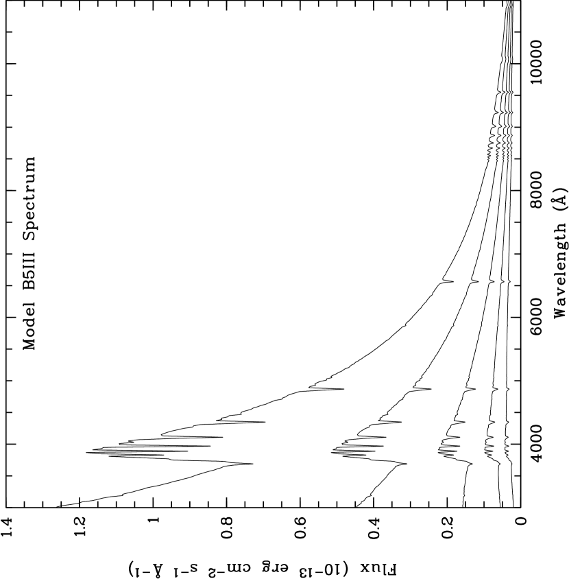
Figure 8: Model spectra of a spectral type B5III star showing the effect of increasing levels of extinction corresponding to $E_{B-V}$ of 0.0 to 0.8 in steps of 0.2.

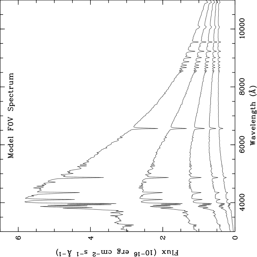
Figure 9: Model spectra of a spectral type F0V star showing the effect of increasing levels of extinction corresponding to $E_{B-V}$ of 0.0 to 0.8 in steps of 0.2.

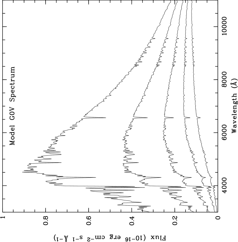
Figure 10: Model spectra of a spectral type G0V star showing the effect of increasing levels of extinction corresponding to $E_{B-V}$ of 0.0 to 0.8 in steps of 0.2.

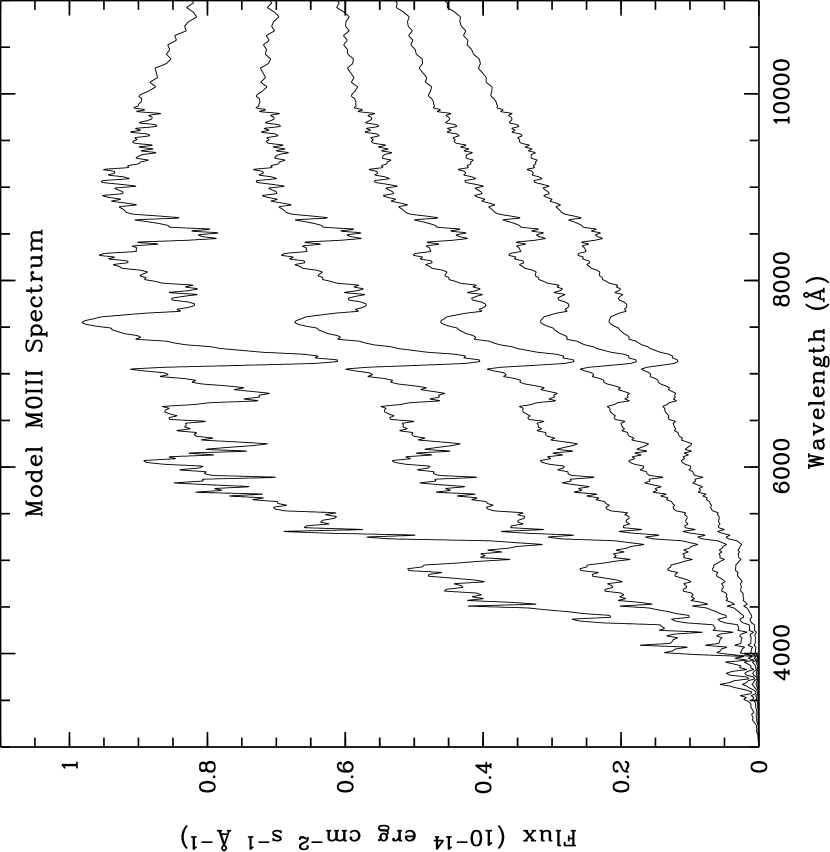
Figure 11: Model spectra of a spectral type M0III star showing the effect of increasing levels of extinction corresponding to $E_{B-V}$ of 0.0 to 0.8 in steps of 0.2.

Figures 8, 9, 10, and 11 show the effect of extinction on observed spectra of various types of stars given in Table 4. There is a significant change in spectral features, such as slope and line strength, from an $E_{B-V}$ value of 0.0 to 0.8. The slope and the features can be used to quantitatively estimate the extinction of the microlensed stars in comparison to the general sample in the Galactic bulge. It is apparent from the model spectra that, although blue stars in the main sequence will always be brighter than red main-sequence stars at all wavelengths, the effects of extinction will cause the stellar population at the far side of the bulge to discriminate against blue stars as source stars in microlensing.

From our previous arguments, we expect a majority of the microlensed sources to show extinction which would correspond to color excess ($E_{B-V}$) values in the range 0.4 to 0.8. Clearly, a collection of microlensed source spectra bearing this characteristic would become statistically significant when estimating the contribution of bulge-bulge lensing to the microlensing optical depth. If this is shown to be statistically the case then this simple method can be used as a statistical distance indicator for microlensed sources.

A knowledge of the distance to the source enables the distance to the lens to be estimated. To demonstrate this, the Galactic bulge model outlined in Section 1.3 shall be used. For a source located at a distance $D_{s}$, the fractional area covered by the Einstein rings of the intervening stars at a depth $dD_{d}$ at a distance $D_{d}$ is

$$A_{f}(D_{d})\,dD_{d}=\frac{4\pi G}{c^{2}}\rho_{0}\exp\left[-\frac{|R_{0}-D_{d}|}{i_{0}}\right]\frac{D_{d}(D_{s}-D_{d})}{D_{s}}\,dD_{d}$$ (34)

As discussed earlier, the probability of the source being microlensed is highest when the source is at the far side of the bulge. The probability distribution of the location of the lenses (in units of the distance to the source) is simply given by $A_{f}(D_{d})$, which is shown in Figure 12. The figure shows that the probability peaks at a distance of $D_{d}=0.85D_{s}$ which, for $D_{s}=9.0\,\mathrm{kpc}$, corresponds to $D_{d}=7.8\,\mathrm{kpc}$. It is worth noting that this does not imply that most of the lenses are at $D_{d}=7.8\,\mathrm{kpc}$. This only implies that if the source is at $D_{s}=9\,\mathrm{kpc}$, a lens distance of 0.85 $D_{s}$ is twice more likely than a lens distance of 0.6 $D_{s}$.

Since the angular Einstein ring radius is known from the characteristic time scale of the event, the extinction exhibited in the spectra of microlensed sources can be used as a means to estimate the size of the Einstein ring radius in terms of AU. Detectable deviations in microlensing light curves due to planetary masses depend highly upon the star-planet distance in the lensing system (Bennett & Rhie, 1996; Gaudi & Sackett, 2000), making this method a useful technique to constrain calculations of planet detection efficiencies.

4 CONCLUSIONS

Various Galactic models have been used to demonstrate the theoretical effects of extinction upon the microlensing optical depth. The exponential density model provides the best approximation of the microlensing optical depth when taking extinction into account. For the exponential model, it is shown that stars that are lensed within Baade’s window are about 13 times more likely to be at the far side of the bulge than the near side. The estimated optical depth is $\approx 4.50\times 10^{-6}$ for $a_{1}=2.0$ and $a_{2}=3.0$, which is comparable to the observed optical depths of $(3.3\pm 1.2)\times 10^{-6}$ and $(3.9_{-1.2}^{+1.8})\times 10^{-6}$ measured by Udalski et al. (1994) and Alcock et al. (1997) respectively.

The calculations presented in this paper do not necessarily assume that there is a onoe-to-one relation between distance and reddening. Rather we assume that the sources will be more reddened than the lens stars and, statistically, other non-microlensed sources in the same narrow field. The follow-up study presented in Kane & Sahu (2003), for example, selects comparison stars which are very close to the microlensed sources so that the angular distance between them, and hence the variation in foreground extinction, is at a minimum.

The effects of extinction on spectra of microlensed sources have been simulated using Kurucz model spectra. It is shown that the majority of microlensed sources should exhibit extinction between $E_{B-V}=0.4$ and $E_{B-V}=0.8$. It is also shown that using extinction as a distance indicator for microlensed sources may be used to statistically estimate the distance to the lens from the probability distribution corresponding to the appropriate Galactic model.

The measured extinctions for the microlensed sources can be used to determine the expected stellar number density gradient $a$ which, in turn, can be used to determine the optical depth more accurately. If there is a smooth velocity gradient within the Galactic bulge, one would expect a statistical correlation between the radial velocity and the extinction of microlensed sources which, given enough samples, will provide useful information regarding the 3-dimensional velocity structure of the far side of the Galactic bulge. Given the variation in extinction through the Galactic bulge, the sample would require $\sim 100$ spectra of microlensed sources in order to clearly show the described effects.

Appendix A FRACTIONAL AREA FOR EXPONENTIAL DENSITY

This appendix details the evaluation of the integral in equation (26). Let the integral be defined as

$$I=\int_{0}^{D_{s}}\exp\left[-\frac{|R_{0}-D_{d}|}{i_{0}}\right]\frac{D_{d}(D_{s}-D_{d})}{D_{s}}\,dD_{d}$$ (A1)

Due to the absolute value of $R_{0}-D_{d}$, this integral is a boundary value problem around the Galactocentric distance $R_{0}$. Hence, the integral needs to be separated into two integrals defined on either of the boundary $R_{0}$, as follows

$$I_{1}=\int_{0}^{D_{s}}\exp\left[-\frac{(R_{0}-D_{d})}{i_{0}}\right]\frac{D_{d}(D_{s}-D_{d})}{D_{s}}\,dD_{d}\\$$

for $D_{s}<R_{0}$, and

$$I_{2} = \int_{0}^{R_{0}}\exp\left[-\frac{(R_{0}-D_{d})}{i_{0}}\right]\frac{D_{d}(D_{s}-D_{d})}{D_{s}}\,dD_{d}$$

$$+\int_{R_{0}}^{D_{s}}\exp\left[-\frac{(D_{d}-R_{0})}{i_{0}}\right]\frac{D_{d}(D_{s}-D_{d})}{D_{s}}\,dD_{d}$$

for $D_{s}>R_{0}$. These two integrals will now be considered separately.

A.1 Source Distance Less Than ${\bf R_{0}}$

The integral $I_{1}$ may be expanded into two parts

$$I_{1}=\int_{0}^{D_{s}}D_{d}\exp\left[-\frac{(R_{0}-D_{d})}{i_{0}}\right]\,dD_{d}-\int_{0}^{D_{s}}\frac{D_{d}^{2}}{D_{s}}\exp\left[-\frac{(R_{0}-D_{d})}{i_{0}}\right]\,dD_{d}$$ (A2)

Both of these integrals may be evaluated using integration by parts:

$$\int u\frac{dv}{dx}\,dx=uv-\int v\frac{du}{dx}\,dx$$

In the case of the first integral, it is most convenient to define

$$u=D_{d}\mbox{ and }\frac{dv}{dD_{d}}=\exp\left[-\frac{(R_{0}-D_{d})}{i_{0}}\right]$$

Then it follows that

$$\frac{du}{D_{d}}=1\mbox{ and }v=\int\exp\left[-\frac{(R_{0}-D_{d})}{i_{0}}\right]\,D_{d}$$

By substituting $\gamma=(R_{0}-D_{d})/i_{0}$, $v$ becomes

$$v = -i_{0}\int e^{-\gamma}\,d\gamma$$

$$= i_{0}e^{-\gamma}$$

$$= i_{0}\exp\left[-\frac{(R_{0}-D_{d})}{i_{0}}\right]$$

Then using integration by parts

$$\int u\frac{dv}{dD_{d}}\,dD_{d} = D_{d}i_{0}\exp\left[-\frac{(R_{0}-D_{d})}{i_{0}}\right]-i_{0}\int\exp\left[-\frac{(R_{0}-D_{d})}{i_{0}}\right]\,dD_{d}$$ (A3)

$$= i_{0}D_{d}\exp\left[-\frac{(R_{0}-D_{d})}{i_{0}}\right]-i_{0}^{2}\exp\left[-\frac{(R_{0}-D_{d})}{i_{0}}\right]$$

$$= i_{0}\exp\left[-\frac{(R_{0}-D_{d})}{i_{0}}\right](D_{d}-i_{0})$$

In the case of the second integral, it is convenient to define

$$u=\frac{D_{d}^{2}}{D_{s}}\mbox{ and }\frac{dv}{dD_{d}}=\exp\left[-\frac{(R_{0}-D_{d})}{i_{0}}\right]$$

Then it follows that

$$\frac{du}{D_{d}}=\frac{2D_{d}}{D_{s}}\mbox{ and }v=i_{0}\exp\left[-\frac{(R_{0}-D_{d})}{i_{0}}\right]$$

Then using integration by parts

$$\int u\frac{dv}{dD_{d}}\,dD_{d} = \frac{D_{d}^{2}}{D_{s}}i_{0}\exp\left[-\frac{(R_{0}-D_{d})}{i_{0}}\right]-\frac{2i_{0}}{D_{s}}\int D_{d}\exp\left[-\frac{(R_{0}-D_{d})}{i_{0}}\right]\,dD_{d}$$ (A4)

$$= i_{0}\frac{D_{d}^{2}}{D_{s}}\exp\left[-\frac{(R_{0}-D_{d})}{i_{0}}\right]-\frac{2i_{0}^{2}}{D_{s}}\exp\left[-\frac{(R_{0}-D_{d})}{i_{0}}\right](D_{d}-i_{0})$$

$$= \frac{i_{0}}{D_{s}}\exp\left[-\frac{(R_{0}-D_{d})}{i_{0}}\right](D_{d}^{2}-2i_{0}D_{d}+2i_{0}^{2})$$

Combining Equation A.3 and Equation A.4 yields

$$I_{1} = \left.i_{0}\exp\left[-\frac{(R_{0}-D_{d})}{i_{0}}\right]\left(D_{d}-i_{0}-\frac{D_{d}^{2}}{D_{s}}+\frac{2i_{0}D_{d}}{D_{s}}-\frac{2i_{0}^{2}}{D_{s}}\right)\right|_{D_{d}=0}^{D_{d}=D_{s}}$$

$$= i_{0}^{2}\exp\left[-\frac{(R_{0}-D_{s})}{i_{0}}\right]\left(1-\frac{2i_{0}}{D_{s}}\right)+i_{0}^{2}\exp\left[-\frac{R_{0}}{i_{0}}\right]\left(1+\frac{2i_{0}}{D_{s}}\right)$$

$$= \frac{i_{0}^{2}e^{-R_{0}/i_{0}}(D_{s}(1+e^{D_{s}/i_{0}})+2i_{0}(1-e^{D_{s}/i_{0}}))}{D_{s}}$$ (A6)

A.2 Source Distance Greater Than ${\bf R_{0}}$

Since the first component of integral $I_{2}$ is identical to integral $I_{1}$ except for the limits, this component may be solved by simply substituting the limits $0\rightarrow R_{0}$ into Equation A.5.

$$I_{2.1} = \left.i_{0}\exp\left[-\frac{(R_{0}-D_{d})}{i_{0}}\right]\left(D_{d}-i_{0}-\frac{D_{d}^{2}}{D_{s}}+\frac{2i_{0}D_{d}}{D_{s}}-\frac{2i_{0}^{2}}{D_{s}}\right)\right|_{D_{d}=0}^{D_{d}=R_{0}}$$ (A7)

$$= i_{0}\left(R_{0}-i_{0}-\frac{R_{0}^{2}}{D_{s}}+\frac{2i_{0}R_{0}}{D_{s}}-\frac{2i_{0}^{2}}{D_{s}}\right)-i_{0}\exp\left[-\frac{R_{0}}{i_{0}}\right]\left(-i_{0}-\frac{2i_{0}^{2}}{D_{s}}\right)$$

$$= \frac{i_{0}(R_{0}D_{s}+2i_{0}R_{0}+i_{0}e^{-R_{0}/i_{0}}(D_{s}+2i_{0})-i_{0}D_{s}-2i_{0}^{2}-R_{0}^{2})}{D_{s}}$$

As was the case for integral $I_{1}$, the second component of integral $I_{2}$ may be solved by expanding the integral into two parts

$$I_{2.2}=\int_{R_{0}}^{D_{s}}D_{d}\exp\left[-\frac{(D_{d}-R_{0})}{i_{0}}\right]\,dD_{d}-\int_{R_{0}}^{D_{s}}\frac{D_{d}^{2}}{D_{s}}\exp\left[-\frac{(D_{d}-R_{0})}{i_{0}}\right]\,dD_{d}$$

Using integration by parts, the first integral becomes

$$I_{2.2.1}=-i_{0}\exp\left[-\frac{(D_{d}-R_{0})}{i_{0}}\right](D_{d}+i_{0})$$ (A8)

and the second integral becomes

$$I_{2.2.2}=-\frac{i_{0}}{D_{s}}\exp\left[-\frac{(D_{d}-R_{0})}{i_{0}}\right](D_{d}^{2}+2i_{0}D_{d}+2i_{0}^{2})$$ (A9)

so that combining Equation A.8 and Equation A.9 yields

$$I_{2.2} = \left.i_{0}\exp\left[-\frac{(D_{d}-R_{0})}{i_{0}}\right]\left(-D_{d}-i_{0}+\frac{D_{d}^{2}}{D_{s}}+\frac{2i_{0}D_{d}}{D_{s}}+\frac{2i_{0}^{2}}{D_{s}}\right)\right|_{D_{d}=R_{0}}^{D_{d}=D_{s}}$$ (A10)

$$= i_{0}\exp\left[-\frac{(D_{s}-R_{0})}{i_{0}}\right]\left(i_{0}+\frac{2i_{0}^{2}}{D_{s}}\right)-i_{0}\left(-R_{0}-i_{0}+\frac{R_{0}^{2}}{D_{s}}+\frac{2i_{0}R_{0}}{D_{s}}+\frac{2i_{0}^{2}}{D_{s}}\right)$$

$$= \frac{i_{0}(i_{0}D_{s}-2i_{0}^{2}+i_{0}e^{-(D_{s}-R_{0})/i_{0}}(D_{s}+2i_{0})+R_{0}D_{s}-2i_{0}R_{0}-R_{0}^{2})}{D_{s}}$$

Combining Equation A.7 and Equation A.10 leads to the expression for integral $I_{2}$

$$I_{2}=\frac{i_{0}\left(2i_{0}^{2}\left(e^{-\frac{D_{s}-R_{0}}{i_{0}}}+e^{-\frac{R_{0}}{i_{0}}}-2\right)-2R_{0}^{2}+D_{s}\left(i_{0}e^{-\frac{D_{s}-R_{0}}{i_{0}}}+i_{0}e^{-\frac{R_{0}}{i_{0}}}+2R_{0}\right)\right)}{D_{s}}$$ (A11)

Table 1: Variation of instantaneous probability of microlensing with extinction $a_{c}$ for a constant density between the observer and the source.

$a_{c}$	$A_{f}(7)N_{obs}(7)/N_{tot}(10^{-7})$	$A_{f}(8)N_{obs}(8)/N_{tot}(10^{-7})$	$A_{f}(9)N_{obs}(9)/N_{tot}(10^{-7})$
1.0	10.92	14.26	18.04
2.0	8.83	10.68	12.51
3.0	7.66	8.85	9.91
4.0	6.87	7.69	8.34
5.0	6.28	6.86	7.26
6.0	5.83	6.24	6.47
7.0	5.46	5.74	5.85

Table 2: Variation of instantaneous probability of microlensing with extinction $a_{c}$ for a constant density for the disk and bulge.

$a_{c}$	$A_{f}(7)N_{obs}(7)/N_{tot}(10^{-7})$	$A_{f}(8)N_{obs}(8)/N_{tot}(10^{-7})$	$A_{f}(9)N_{obs}(9)/N_{tot}(10^{-7})$
1.0	3.54	5.80	10.22
2.0	4.91	4.02	3.54
3.0	5.83	3.19	1.87
4.0	6.54	2.68	1.18
5.0	7.12	2.33	0.82
6.0	7.61	2.08	0.61
7.0	8.03	1.88	0.47

Table 3: Variation of instantaneous probability of microlensing with extinction $a_{2}$ for an exponential density model and $a_{1}=1$.

$a_{2}$	$A_{f}(7)N_{obs}(7)/N_{tot}(10^{-6})$	$A_{f}(8)N_{obs}(8)/N_{tot}(10^{-6})$	$A_{f}(9)N_{obs}(9)/N_{tot}(10^{-6})$
1.0	0.48	2.02	6.07
2.0	0.56	2.35	3.52
3.0	0.60	2.51	2.52
4.0	0.62	2.62	1.97
5.0	0.64	2.70	1.62
6.0	0.65	2.76	1.38
7.0	0.66	2.80	1.20

Table 4: Characteristics of example spectral types

Spectral Type	$T_{eff}$	$\log g$	$m_{V}$
M0III	3800	+1.34	14.4
G0V	6030	+4.39	19.2
F0V	7200	+4.34	17.4
B5III	15000	+3.49	12.4

Figure 1: Schematic of the geometry used in the Galactic model assuming that all the microlensed sources are within the bulge.

Figure 2: Probability that a given microlensed source is at a distance $D_{s}$ as a function of $D_{s}$, for values of $a_{c}$ ranging from $a_{c}=1$ (uniform density of observed stars) to $a_{c}=10$.

Figure 3: Optical depth as a function of $a_{c}$, which is the ratio of the maximum to the minimum observed stellar number density in a given line of sight, assuming a constant matter density for the lenses.

Figure 4: Probability that a given microlensed source is at a distance $D_{s}$ as a function of $D_{s}$, for values of $a_{c}$ ranging from $a_{c}=1$ (uniform density of observed stars) to $a_{c}=10$.

Figure 5: Optical depth as a function of $a_{c}$, which is the ratio of the maximum to the minimum observed stellar number density in a given line of sight, assuming that the matter density for the lenses is constant in the disk and in the bulge.

Figure 6: Probability that a given microlensed source is at a distance $D_{s}$ as a function of $D_{s}$, for values of $a_{2}$ ranging from $a_{2}=a_{1}$ to $a_{2}=10$. This has been calculated for (a) $a_{1}=1$, (b) $a_{1}=2$, (c) $a_{1}=5$, and (d) $a_{1}=10$ with the restriction as expected from physical grounds that $a_{1}<a_{2}$.

Figure 7: Optical depth as a function of $a_{2}$, which is the ratio of the maximum to the minimum observed stellar number density in a given line of sight, assuming an exponential matter density for the lenses. This has been calculated for $a_{1}=1$, $a_{1}=2$, and $a_{1}=5$ with the restriction as expected from physical grounds that $a_{1}<a_{2}$.

Figure 12: A probability distribution for lenses given a source located at a distance of $D_{s}=9.0\,\mathrm{kpc}$. In this case, it is most probable that the lens will be located at a distance of $D_{d}=7.8\,\mathrm{kpc}$.

References

- Afonso et al. (2003) Afonso, C., et al. 2003, A&A, 404, 145
- Alcock et al. (1997) Alcock, C., et al. 1997, ApJ, 479, 119
- Alcock et al. (2000a) Alcock, C., et al. 2000, ApJ, 541, 734
- Alcock et al. (2000b) Alcock, C., et al. 2000, ApJ, 552, 582
- Arp (1965) Arp, H. 1965, ApJ, 141, 43
- Beichman et al. (1985) Beichman, C.A., Neugebauer, G., Habing, H.J., Clegg, P.E., & Chester, T.J., 1985, IRAS Explanatory Supplement, published by JPL, Pasadena
- Bennett & Rhie (1996) Bennett, D.P. & Rhie, S.H. 1996, ApJ, 472, 660
- Binney et al. (1991) Binney, J. J., Gerhard, O. E., Stark, A. A., Bally, J., & Uchida, K. I. 1991, MNRAS, 252, 210
- Binney, Bissantz, & Ortwin (2000) Binney, J., Bissantz, N. & Ortwin, G., 2000, ApJ, 537, L99
- Blitz & Spergel (1991) Blitz, L. & Spergel,D. 1991, ApJ, 379, 631
- Di Stefano & Esin (1995) Di Stefano, R. & Esin, A.A. 1995, ApJ, 448, L1
- Dominik & Sahu (2000) Dominik, M. & Sahu, K.C. 2000, ApJ, 534, 213
- Dwek et al. (1995) Dwek, E., et al. 1995, ApJ, 445, 716
- Gaudi & Sackett (2000) Gaudi, B.S. & Sackett, P.D. 2000, ApJ, 528, 56
- Gerhard (2000) Gerhard, O. 2000, in Disk Galaxies and Galaxy Disks, ASP Conf. Ser., in press (astro-ph/0010539)
- Hammersley et al. (2000) Hammersley, P.L., Garzon, F., Mahoney, T.J., Lopez-Corredoira, M., & Torres, M.A.P., 2000, MNRAS, 317, L45
- Kane & Sahu (2003) Kane, S.R. & Sahu K.C. 2003, ApJ, 582, 743
- Kent (1987) Kent, S. 1987, AJ, 93, 1062
- Kiraga & Paczyński (1994) Kiraga, M. & Paczyński, B. 1994, ApJ, 430, L101
- Kroupa, Tout, & Gilmore (1993) Kroupa, P., Tout, C.A., & Gilmore, G. 1993, MNRAS, 262, 545
- Kurucz (1993) Kurucz, R. 1993, ATLAS9 Stellar Atmosphere Programs and 2 km/s grid. Kurucz CD-ROM No. 13. Cambridge, MA: Smithsonian Astrophysical Observatory
- Paczyński (1991) Paczyński, B. 1991, ApJ, 371, L63
- Paczyński et al. (1994) Paczyński, B., et al. 1994, ApJ, 435, L113
- Popowski et al. (2000) Popowski, P., et al. 2000, in Microlensing 2000: A New Era of Microlensing Astrophysics, ASP Conf. Ser. Ed. J.W. Menzies and P.D.Sackett, in press (astro-ph/0005466)
- Sahu (1994a) Sahu, K.C. 1994a, PASP, 106, 942
- Sahu (1994b) Sahu, K.C. 1994b, Nature, 370, 275
- Seaton (1979) Seaton, M.J. 1979, MNRAS, 187, 73p
- Stanek (1995) Stanek, K.Z. 1995, ApJ, 441, L29
- Stanek (1996) Stanek, K.Z. 1996, ApJ, 460, L37
- Sumi et al. (2003) Sumi, T., et al. 2003, ApJ, 591, 20
- Udalski et al. (1994) Udalski, A., et al. 1994, Acta Astron., 44, 165
- Udalski et al. (2000) Udalski, A., et al. 2000, Acta Astron., 50, 1
- Whitelock, Feast, & Catchpole (1991) Whitelock, P., Feast, M. & Catchpole, R. 1991, MNRAS, 248, 276
- Wielen, Jahreiss, & Krüger (1983) Wielen, R., Jahreiss, H., & Krüger, R. 1983, in IAU Colloq. 76, The Nearby Stars and the Stellar Luminosity Function, ed. A.G. Davis Philip & A.R. Upgren (Schenectady: Davis), p.163
- Weinberg (1992) Weinberg, D. 1992, ApJ, 384, 81
- Woźniak & Paczyński (1997) Woźniak, P. & Paczyński, B. 1997, ApJ, 487, 55
- Zhao, Spergel, & Rich (1995) Zhao, H., Spergel, D.N., & Rich, R.M. 1995, ApJ, 440, L13
- Zhao (2000) Zhao, H. 2000, ApJ, 530, 299