Measuring Cluster Temperature Profiles with XMM/EPIC ^,

Using the PV observation of A1795, we illustrate the capability of XMM-EPIC to measure cluster temperature profiles, a key ingredient for the determination of cluster mass profiles through the equation of hydrostatic equilibrium. We develop a methodology for spatially resolved spectroscopy of extended sources, adapted to XMM background and vignetting characteristics. The effect of the particle induced background is discussed. A simple unbiased method is proposed to correct for vignetting effects, in which every photon is weighted according to its energy and location on the detector. We were able to derive the temperature profile of A1795 up to 0.4 times the virial radius. A significant and spatially resolved drop in temperature towards the center ($r<200\leavevmode\nobreak\ {\rm kpc}$) is observed, which corresponds to the cooling flow region of the cluster. Beyond that region, the temperature is constant with no indication of a fall-off at large radii out to $1.2$ Mpc.

1 Introduction

The determination of the temperature profiles of the hot gas in galaxy clusters is essential to derive the gas entropy distribution and to measure the total mass content, through the equation of hydrostatic equilibrium. These are key quantities for cosmological studies based on the properties of galaxy clusters. The baryonic mass fraction in clusters is a strong constraint on the density parameter of the Universe $\Omega$ (Briel, Henry & Böhringer briel1 (1992); White et al. white1 (1993)). If the mass–temperature relation is well calibrated, the mass distribution function and its evolution can be derived from the observed temperature function. This is an independent and powerful probe of $\Omega$, as well as, the index and normalization of the power spectrum of primeval fluctuations (e.g. Oukbir & Blanchard oukbir (1997)). Furthermore, the physics of structure formation and evolution can be assessed. For example, the total mass profile gives information on the physics of gravitational collapse. Current numerical simulations under a cold dark matter scenario predict a universal dark matter profile (Navarro, Frenk & White NFW (1997)). The gas entropy distribution, the relative distribution of the gas and dark matter and departures from self-similarity constrain the thermo-dynamical history of the hot gas and the importance of additional non-gravitational effects, such as galaxy feedback (e.g. Ponman, Cannon & Navarro ponman (1999)).

While gas density profiles have been determined with good accuracy by ROSAT, the shape of the temperature profiles in clusters, as measured by ASCA and SAX, is still a matter of debate (Markevitch et al. markevitch (1998); Irwin et al. irwin1 (1999); White white2 (2000); Irwin & Bregman irwin2 (2000); Molendi et al. molendi (2000); Ettori et al. ettori (2000)). It is at present unclear if cluster atmospheres are essentially isothermal or if the temperature decreases with radius (as expected from numerical simulations of cluster formation). As a result, total mass estimates are typically uncertain by a factor of two (Neumann & Arnaud neumann1 (1999); Horner, Mushotzky & Scharf horner (1999)) and the mass profiles are too uncertain to provide any real constraint on theoretical models.

Figure 1: The total EPIC/MOS1 count rate in the $[10-12]$ keV energy band as a function of time.

Significant progress was expected with XMM-Newton/EPIC (Jansen et al. jansen (2001), Turner et al. turner (2001)), which has a much better sensitivity than ASCA and SAX and does not suffer from the large energy dependent PSF of ASCA, a major source of systematic uncertainty. In this paper, we illustrate the capability of XMM-Newton to measure cluster temperature profiles, using the PV observation of A1795. A1795 is a bright cluster ($S_{\rm X}[2-10]{\rm\ keV}>5\times 10^{-11}\leavevmode\nobreak\ {\rm ergs/s/cm^{2}}$. Its redshift ($z=0.063$) allows a significant coverage of the cluster by the XMM-Newton field of view ($15^{\prime}$ in radius which corresponds to $1.48\leavevmode\nobreak\ {\rm h_{50}^{-1}\leavevmode\nobreak\ Mpc}$ or about 0.5 times the cluster virial radius). The paper is organized as follows: after this introduction, Section 2 presents a methodology for spectro-imagery adapted to XMM background and vignetting characteristics. Our results in term of cluster global properties and temperature profiles are presented in Section 3, with particular emphasis on the various sources of errors. Section 4 contains our conclusions.

2 Data Analysis

A1795 was observed for $\sim 50$ ksec in Revolution 100 in Full Frame Mode with the EPIC/MOS and pn camera. We focus here on the MOS data. We generated calibrated event files with SASv4.1, except for the gain correction. Correct PI channels are obtained by interpolating gain values obtained from the observations of the on-board calibration source closest in time to A1795 observation. Data were also checked to remove any remaining bright pixels. Spectra in various regions were extracted to study temperature variations. Only events corresponding to detector regions in view of the sky are considered (using SASv4.1). The region corresponding to the bright point source in the south was also excluded. A proper treatment of the background and vignetting effects are essential when analyzing extended sources like cluster of galaxies. This is discussed in the following two sections.

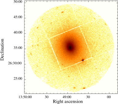
Figure 2: Combined EPIC/MOS1&2 image of A 1795 in the $[0.3-10]{\rm\ keV}$ energy band (logarithmic intensity).

2.1 Background

The XMM background shows considerable variations with time, with flares of various durations and intensities. As an example, we show in Fig. 1 the count rate in the $[10-12]$ keV energy band, where the emission is dominated by the background, due to the small effective area of XMM-Newton/EPIC/MOS in this band. It is essential to remove these periods of high background, which are induced by soft protons from solar flares collected by the telescopes. Not only is the S/N highly degraded, especially at high energy (where the data are crucial for kT measurements), but it is impossible to properly subtract the background, since its spectrum is varying with time. We thus removed all frames corresponding to a count rate greater than 15 ct/100s in the $[10-12]$ keV band. After this data cleaning, the useful observing time for MOS1 and MOS2 is 32.1 ksec and 32.3 ksec, respectively. The corresponding EPIC/MOS1&2 image in the $[0.3-10]{\rm\ keV}$ energy band is shown on Fig.2. The remaining background is dominated by the cosmic X–ray background at low energy and the Cosmic Ray (CR) induced background at energies above typically 1.5 keV.

To estimate the background we used the Lockman Hole (LH) observations made with the thin filter (Rev 70 and Rev 73 for MOS1 and Rev 71 for MOS2). Data were filtered for high background and regions corresponding to the 10 brightest sources were excluded.

It is known that the CR induced background changes slightly in the FOV. It is thus better to consider the same extraction regions in detector coordinates for the source and the background. Figure 3 shows the raw cluster spectrum in the $4.5^{\prime}-5^{\prime}$ region, the background spectrum derived from the LH observation and the corresponding background subtracted spectrum. Note the Al and Si fluorescence lines in the background spectrum and the very hard continuum above 2 keV typical of CR induced background. As a result, even for a bright cluster like A1795 and relatively close to the center, the background dominates the emission at high energies (here above 7 keV). This is an important limitation for temperature estimation.

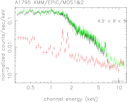
Figure 3: Summed EPIC/MOS1 and MOS2 spectra in the $4.5^{\prime}-5^{\prime}$ region. Green points: raw spectrum. Red points: the background spectrum derived from the LH observation. Black points: the corresponding background subtracted cluster spectrum.

The CR induced background changes slightly with time: the average background level obtained after flare cleaning varies typically by less than $10\%$ from observation to observation. We considered two criteria for background normalization (with each camera treated independently): the count rate in the $[10-12]$ keV band in the FOV (where sky X–ray emission is negligible) and the count rate in the $[0.3-12]$ keV band in the region of the detector masked by the proton shield (no sky emission). The derived normalization factor between the LH and A1795 observations varies from 0.94 to 1.03 depending on the camera and criteria considered. In the following we use a nominal a normalization factor of unity. It will be varied by $\pm 5\%$ to assess systematic uncertainties due to background subtraction.

Note that this treatment allows a proper estimate of the CR induced background, but not of the soft X-ray diffuse background (which varies with position on the sky) and of the extra-galactic background (which depends on the absorbing hydrogen column density along the line of sight). However, the source usually dominates the background except at high energy (Fig 3) and we are mostly sensitive to CR induced background. Furthermore, $N_{H}$ values are similar in the directions toward A1795 and LH and we checked from ROSAT survey maps (Snowden et al. snowden1 (1995),snowden2 (1997)) that the X-ray emission around the LH and A1795 in the soft band ($[0.4-1.2]$ keV) differ by less than $30\%$ on average.

2.2 Correction for vignetting effects

2.2.1 Methodology

While the XMM-Newton/MOS spectral resolution does not show spatial variations, the effective area at a given energy does depend on position. This effect has to be taken into account in modeling spectra extracted from various regions. The exact method is to perform a convolution of a source model with the instrument response (i.e. point by point) and to compare the resulting modeled spectrum with the observed spectrum of the chosen region. This method is complex to implement, especially if the region under consideration is not assumed to be isothermal. In any case, it requires an a priori model for the source spatial distribution.

A simpler and widely used method is to use the emission weighted effective area in the region, derived from the observed global photon spatial distribution (the same weighting is done at each energy). The incident source spectrum is simply compared with the observed spectrum using this effective area (ARF). This method has severe drawbacks. First, it introduces extra noise, since the observed photon distribution used in the ARF average is noisy. Taking this error into account is not trivial. Even more important, the method introduces a bias in the determination of the spectral parameters. Since the effective area decreases with distance from the center, the detected distribution of photons (at a given energy or integrated over the energy band) is always more pronounced towards the center than the source distribution (the well known distortion of the observed image with respect to the incident image). If the average of the effective area is done using the observed distribution, too much weight is given to the central regions. The overall effective area is thus overestimated. Moreover since the variation with energy of the effective area depends on position (the effective area decreases more rapidly with distance for high energy photons than for low energy ones), a bias is introduced. The overestimate of the effective area is higher at high energy than at low energy. The resulting effect is that the fit for the temperature is biased to lower values.

We propose instead the following method, which is easy to implement, does not introduce bias and does not require any a priori assumptions about the spatial variation of the source (either in intensity or in spectroscopic properties). When extracting the spectrum of a region $Reg$, we weight each photon with energy $E_{I}$ falling at position $(x_{j},y_{j})$ by the ratio of the effective area at that position $A_{x_{j},y_{j}}(E_{I})$ to the central effective area $A_{0,0}(E_{I})$. We can thus define a ‘corrected’ spectrum C(I), where C is the corrected photon counts in channel I centered on $E_{I}$ with width $\Delta E_{I}$:

$$C(I) = \sum_{j}w_{j};\leavevmode\nobreak\ (x_{j},y_{j})\in Reg;$$

$$\leavevmode\nobreak\ \leavevmode\nobreak\ \leavevmode\nobreak\ \leavevmode\nobreak\ \leavevmode\nobreak\ \leavevmode\nobreak\ \leavevmode\nobreak\ \leavevmode\nobreak\ \leavevmode\nobreak\ \leavevmode\nobreak\ \leavevmode\nobreak\ \leavevmode\nobreak\ E_{I}-\Delta E_{I}/2<E_{j}<E_{I}+\Delta E_{I}/2$$

$$w_{j} = \frac{A_{0,0}(E_{I})}{A_{x_{j},y_{j}}(E_{I})}$$ (2)

This weighting factor has to be taken into account in the error estimate. The variance on $C(I)$ is

$$\sigma^{2}(C(I))=\sum_{j}w_{j}^{2}$$ (3)

Note that this method corresponds to CORRECT mode in EXSAS for ROSAT data reduction (Zimmermann et al. zimmermann (1998)). This ‘corrected’ spectrum is an estimate of the spectrum one would get if the detector were flat. It can thus be compared with the total spectrum of the source given by the model, convolved with the instrument response at the center of the detector. The method is exact for an instrument with perfect spatial and spectral ($\Delta E$) resolution, i.e., the energy and position of the detected photons correspond exactly to those of the emitted photons. However, the method cannot introduce significant bias as long as the vignetting effect is small at the scale of the PSF and remains the same for energies differing by about $\Delta E$. This is certainly the case for XMM-Newton. Its only drawback, as compared to the direct exact method, is a degradation of the statistical quality: the relative error is increased by a factor $\sqrt{\langle{w_{j}^{2}}\rangle}/\langle{w_{j}}\rangle$ where the brackets denote the average over the photons in a given energy bin I. This is not a problem if the effective area does not vary much in the region being considered ($\sqrt{\langle{w_{j}^{2}}\rangle}/\langle{w_{j}}\rangle\sim 1$).

For consistency, the background spectra were obtained using the same correction method as for the source. The CR-induced background component is not vignetted, but, since we extract the background and source spectra from the same region in detector coordinates, the correction factor is the same and thus cancels.

2.2.2 Vignetting data

For the vignetting function of the telescope, we used the data available on the XMM-Newton home page in August 2000, based on a simplified model of the mirrors. Data in the SASv4.1 CCF are wrong and correct values derived from the last model implemented in SciSim were only made available after the completion of this work. We add the vignetting effect due to the obscuration by the Reflection Grating Array (RGA), as derived from SciSim (P.Gondoin private communication). This effect can be supposed to be energy independent but introduces an azimuthal dependence in the vignetting function. The overall vignetting is in reasonable agreement with values derived from a comparison of on- and off-axis (10’ from centre) observations of the supernova remnant G21.5$-$0.9 (Neumann, 2000).

2.3 Spectral fitting

The source spectra (with errors) computed as described above, are binned so that the S/N ratio is greater than 3 $\sigma$ in each bin after background subtraction. The spectra are fitted with XSPEC using a MEKAL model (Mewe et al. mewe1 (1985),mewe2 (1986); Kaastra kaastra (1992); Liedahl et al. liedahl (1995)). Since the spectra are ‘corrected’ we can use the on axis response file. Note that the response matrix we used (version v3.15) assumes no energy dependence for the RGA transmission. Only data above 0.3 keV are considered due to remaining uncertainties in the MOS response below this energy.

3 Results

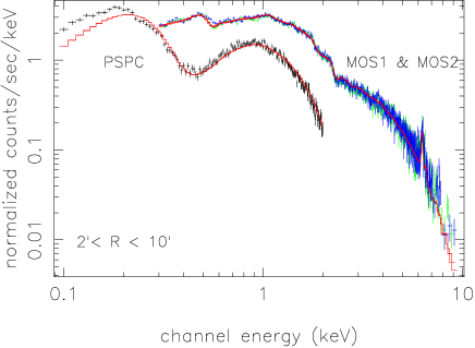
Figure 4: XMM and ROSAT spectra of the cluster from the region covering radii of $2^{\prime}-10^{\prime}$. Green (blue) points: EPIC/MOS1(2) data. Black points: PSPC data. The EPIC spectra are background subtracted and corrected for vignetting as described in Sec. 2. The red line is the best fit isothermal model with ${\rm k}T=5.95\leavevmode\nobreak\ {\rm\ keV}$, an abundance of 0.27 times the solar value and a relative normalization between the EPIC and PSPC data of 1.05.

3.1 Overall spectrum

The overall MOS1 and MOS2 spectra, within $10^{\prime}$ of the cluster center, excluding the central $R<2^{\prime}$ cooling flow region (see below) is shown in Fig. 4. The spectra are corrected for vignetting and background subtracted as described above. They are compared with the PSPC spectrum of the same region. As the PSPC FOV is much larger, the background spectrum can be reliably estimated from the outer region ($25^{\prime}-42^{\prime}$), free of cluster emission. The XMM-Newton and PSPC data are jointly fitted in the $[0.3-10]$ keV range. We let the relative normalization between the various instruments be free but assumed a common temperature and abundance. When the $N_{\rm H}$ value is frozen to the 21 cm value ($N_{\rm H}=1.05\times 10^{20}\leavevmode\nobreak\ {\rm cm^{-2}}$; Mittaz, Lieu & Lockman mittaz (1998)), the best fit gives ${\rm k}T=5.95\pm 0.1$ keV and an abundance of $0.27\pm 0.02$. The reduced $\chi^{2}$ is $1.27$. If the $N_{\rm H}$ value is allowed to be free, we derive $N_{\rm H}=0.95\pm 0.07\times 10^{20}\leavevmode\nobreak\ {\rm cm^{-2}}$, in agreement with the 21 cm value and the $\chi^{2}$ value, temperature and abundance are unchanged. In the following we thus fix the $N_{\rm H}$ value to the 21 cm value.

The reduced $\chi^{2}$ is reasonable, the deviations between model and data are less than typically $10\%$. One should also note the excellent consistency between the MOS1 and MOS2 spectra (relative normalization of 1.02) and between the PSPC and XMM (relative normalization of 1.05) The best fit overall temperature in this region is in good agreement with the global temperature value from ASCA ($6.0\pm 0.3{\rm\ keV}$, Markevitch et al. markevitch (1998)) and SAX ($6.0\pm 0.4{\rm\ keV}$, Irwin & Bregman irwin2 (2000)). Overall this suggests that the data processing and the on-axis response matrix are reasonable.

When the best fit model is extrapolated down to 0.1 keV, the known soft excess in the EUVE data below 0.2 keV (Mittaz, Lieu & Lockman mittaz (1998)) is clearly apparent in the PSPC spectrum. This excess cannot be yet studied with XMM, due to the previously mentioned calibration uncertainties (Section 2.3) in the response matrix in the $[0.15-0.3]$ keV range.

Figure 5: Comparison of XMM (open circles) and PSPC (full line) surface brightness profiles. The profiles are background subtracted and corrected for vignetting (see text for details). The PSPC data are renormalized to the total number of XMM counts in the $2^{\prime}$ to $10^{\prime}$ region. Insert: zoom of the region where the discrepancy is maximum. Note the excellent agreement in shape.

3.2 Surface brightness profile

An independent check of the background subtraction and vignetting correction was performed by comparing XMM and PSPC surface brightness profiles. The PSPC profile in the $[0.9-2.]$ keV energy range was extracted and corrected for vignetting using the standard EXSAS procedure for deriving exposure maps. As was done in the spectral analysis, the background was estimated from outer regions in the FOV with point sources removed. The PSPC profile is compared in Fig. 5 with the vignetting-corrected summed MOS1 and MOS2 profile in the $[1-3]$ keV band. The energy bands were chosen so that the relative emissivity between XMM and the PSPC were insensitive to possible temperature gradients, while at the same time retaining a good S/N ratio. The XMM background profile was estimated from the Lockman Hole data. The profiles are binned so that there is at least a $5\leavevmode\nobreak\ \sigma$ detection in each bin. For direct comparison the PSPC data in the figure were renormalized to the total XMM counts over radii from $2^{\prime}$ to $10^{\prime}$. The agreement in shape is excellent up to $15^{\prime}$ with the maximum difference (at the $25\%$ level only) occurring at radii between $8^{\prime}$ and $11^{\prime}$. This comparison further validates our data analysis method.

Figure 6: Comparison of the temperature derived from EPIC/MOS1 and MOS2 data for the various rings of the radial temperature profile. The errors are at the $90\%$ confidence level.

3.3 Radial temperature profile

Spectra in concentric rings (i.e., annuli) centered on the cluster X–ray emission peak were extracted from MOS1 and MOS2 data. We tried to attain roughly similar precision in the temperature estimates from region to region. Thus the widths of the various rings were chosen so that at least a $5\sigma$ detection in the $[5-10]$ kev range was reached. This was possible for all but the final annulus. In addition a minimum width of $30^{\prime\prime}$ was set corresponding to the $90\%$ encircled energy radius of the PSF. Each vignetting-corrected and background-subtracted spectrum was fitted with an isothermal MEKAL model allowing the normalization, temperature and abundance to be the only free parameters.

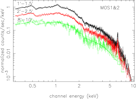
Figure 7: Combined EPIC/MOS1&2 spectra of the inner $1^{\prime}-1.5^{\prime}$ region (black points), the $2^{\prime}-2.5^{\prime}$ region just outside the cooling flow region (red points) and the outer $8^{\prime}-10^{\prime}$ ring (green points). The full lines are the best fit isothermal model for each region.

The temperatures determined from the MOS1 and MOS2 data are mutually consistent (see Fig. 6). We thus summed the MOS1 and MOS2 data and re-determined the temperature in each ring from the combined data. The fits are good with reduced $\chi^{2}$ values in the range $0.98-1.24$. The worst $\chi^{2}$ value corresponds to the central rings, where we are affected by the cooling flow. Typical spectra are shown in Fig. 7: the inner $1^{\prime}-1.5^{\prime}$ region, the $2^{\prime}-2.5^{\prime}$ region just outside the cooling flow region and the last ring ($8^{\prime}-10^{\prime}$ region). The errors in our temperature estimates consist of the quadratic sum of the statistical error (at the $90\%$ confidence level) and systematic errors estimated by varying the background level by $\pm 5\%$. We also fitted the spectra in the restricted $0.3-7$ keV range, which is less sensitive to background and we did not obtain any significant differences in the derived temperatures. We also tentatively estimate the temperature in an outer region covering radii of $10^{\prime}-12^{\prime}$. The temperature from this region is uncertain and the value should be used with caution. The fit is not good ($\chi^{2}=1.8$), due to an excess at energies above 5 kev and a poor fit at low energies. Both effects are likely due to uncertainties in the background (both the X-ray background at low energies and CR-induced background at high energies) which dominates the emission. The error includes systematic errors estimated by varying the background level by $\pm 5\%$ and restricting the fit to the $[0.3-5]$ keV energy range.

The resulting temperature profile is shown in Fig. 8 as a function of radius both in physical units (upper axis) and scaled by the virial radius (bottom axis). The scaled radius is defined as r/$r_{200}$ where $r_{\rm 200}=2.76\,{\rm Mpc}$ is the virial radius for a $6{\rm\ keV}$ cluster at $z=0.063$ (Evrard et al. evrard (1996)).

Figure 8: Radial temperature profile as a function of angular radius (upper axis) and scaled radius (lower axis), derived from XMM/EPIC data. The horizontal line corresponds to the mean value derived from fitting the overall spectrum of the region from $2^{\prime}$ to $10^{\prime}$ radius. The dotted line is the universal profile derived by Markevitch et al. (markevitch (1998)) from ASCA data, normalized to the virial radius and mean temperature of A1795.

4 Conclusion

We have determined the temperature profile of A1795 up to a typical radius 0.4 times the virial radius. Both vignetting effects and background subtraction are reasonably well understood. The temperature profile can be compared with the profile derived by SAX (Irwin & Bregman irwin2 (2000)) and ASCA (Markevitch et al. markevitch (1998)). The dramatic improvement in accuracy and spatial resolution of the profiles must be noticed. However, our results show that the limiting factor for determining temperature profiles with XMM is the high level of the CR-induced background. Improvement of background models would be of great help.

The drop of temperature in the center as measured by ROSAT (Briel and Henry 1996), but not seen with SAX, is unambiguously confirmed. The drop in temperature is also readily apparent in the spectrum of the central region shown in Fig.7, which shows the increasing importance of the Fe L line complex. Moving in toward the cluster center the temperature starts to drop at about $2^{\prime}$; further in the temperature profile is, for the first time, well resolved. A significant excess in the surface brightness profile (as compared to the overall $\beta$ model) is also observed in the same region (Briel & Henry briel2 (1996)). This temperature drop indicates that the gas is cooling. A detailed study of this inner region, based on both EPIC and RGS data, can be found in Tamura et al. (tamura (2001)).

Beyond $2^{\prime}$ the temperature results are consistent with an isothermal profile at the mean temperature (full line in Fig.8) in agreement with SAX results. The ASCA temperature beyond $6^{\prime}$ (Markevitch et al. markevitch (1998)) is also in excellent agreement with our data, but is significantly higher in the $1.5-6^{\prime}$ radial range (k$T=8.2^{+1.6}_{-1.5}{\rm\ keV}$). The temperature in the central $r<1.5^{\prime}$ region is corrected for the presence of the cooling flow and cannot be directly compared with our data. We also show in Fig.8 the decreasing ‘universal’ profile obtained by Markevitch et al. (markevitch (1998)) from their compilation of ASCA temperature profiles (dotted line). It can be safely compared to our data outside the cooling flow region. Our results do not support this type of profile for A1795. However, we emphasize that no definitive conclusion should be drawn yet, based on the observation of one cluster only and while we are still in the early phases of the XMM mission. In particular we have assumed that the (small) energy dependence in the shape of the PSF can be neglected. This still needs to be confirmed with in-flight calibration data and detailed simulations.

- (1) Briel U. G., Henry J. P., Böhringer H., 1992, A&A, 259, L31
- (2) Briel U.G., Henry J.P., 1996, ApJ, 472, 131
- (3) Horner D.J., Mushotzky R.F., Scharf C.A., 1999, ApJ, 520, 78
- (4) Ettori S., Bardelli S., De Grandi S., Molendi S., Zamorani G., Zucca E., 2000, MNRAS, 318, 239
- (5) Evrard A.E., Metzler C.A., Navarro J.F., 1996, ApJ, 469, 494
- (6) Irwin J.A., Bregman J.N., Evrard A.E., 1999, ApJ, 519, 518
- (7) Irwin J.A., Bregman J.N., 2000, ApJ, 538, 543
- (8) Jansen, F., Lumb, D., Altieri, B. et al. 2001, A&A, 365 (this issue)
- (9) Kaastra J.S., 1992, An X-ray spectral Code for Optically Thin Plasmas, Internal SRON-Leiden Report, updated version 2.0
- (10) Tamura T., Kaastra J.S., Petreson J.R., et al. 2001, A&A, 365 (this issue)
- (11) Liedahl, D.A., Osterheld, A.L., and Goldstein, W.H. 1995, ApJL, 438, 115
- (12) Markevitch M., Forman W.R., Sarazin C.L., Vikhlinin A., 1998, ApJ, 503, 77
- (13) Mewe, R., Gronenschild, E.H.B.M., and van den Oord, G.H.J. 1985, A&AS, 62, 197
- (14) Mewe, R., Lemen, J.R., and van den Oord, G.H.J. 1986, A&AS, 65, 511
- (15) Molendi S., De Grandi S., Fusco-Femiano R., ApJ, 2000, 533, L43
- (16) Mittaz J., Lieu R., Lockman F., 1998, ApJ 498, L17
- (17) Navarro J.F., Frenk C.S., White S.D.M., 1997, ApJ, 490, 493
- (18) Neumann D.M., Arnaud M., 1999, A&A, 348, 711
- (19) Neumann D.M., 2000, Report on the in-flight vignetting calibration of the MOS cameras aboard the XMM NEWTON satellite, CEA/Saclay, France http://xmm.vilspa.esa.es/calibration/
- (20) Oukbir J., Blanchard A., 1997, A&A, 317, 1
- (21) Ponman T.J., Cannon D.B., Navarro J.F., 1999, Nature, 397, 135;
- (22) Snowden S.L. , Freyberg M. J., Plucinsky P. P. et al. 1995, ApJ, 454, 643
- (23) Snowden S.L., Egger R., Freyberg M. J. et al. , 1997, ApJ, 485, 125
- (24) Turner, M.J.L., Abbey, A., Arnaud, M. et al. 2001, A&A, 365 (this issue)
- (25) White S.D.M., Navarro J.F., Evrard A.E., Frenk C.S., 1993, Nat. 366, 429
- (26) White D.A., 2000, MNRAS, 312, 663
- (27) Zimmermann U., Boese G., Becker W., Belloni T., Döbereiner S., Izzo C., Kahabka P., Schwentker O., 1998, EXSAS User’s Guide MPE Report ROSAT Scientific Data Center