CMB Anisotropies in Pre-Big Bang Cosmology

Abstract

We present an alternative scenario for cosmic structure formation where initial fluctuations are due to Kalb-Ramond axions produced during a pre-big bang phase of inflation. We investigate whether this scenario, where the fluctuations are induced by seeds and therefore are of isocurvature nature, can be brought in agreement with present observations by a suitable choice of cosmological parameters. We also discuss several observational signatures which can distinguish axion seeds from standard inflationary models.

Introduction

The pre-big bang idea (see PBB and references therein) represents one of the first and most interesting attempts to develop a new cosmological scenario which solves the horizon and flatness problems, based on string theory. In this radically new picture, the underlying duality symmetry present in the low energy sector of string theory naturally leads to an inflationary phase prior to the big bang during which curvature and dilaton are growing.

Superstring theory is a tensor-scalar theory of gravity in 10 dimensions. The minimal low energy effective action of the NS-NS sector of string theory can be written under certain conditions as

$$S=\int d^{4}x\sqrt{|g|}e^{-\phi}\left[\mbox{R}+(\nabla\phi)^{2}-3(\nabla\log b)^{2}-\frac{1}{2}e^{2\phi}(\nabla\sigma)^{2}\right],$$ (1)

where we have assumed dimensional reduction by compactification of 6 dimensions on some isotropic Ricci flat manifolds. This action includes a time dependent dilaton field $\phi(t)$. R is the Ricci scalar of the 4-dimensional metric $g_{\mu\nu}=\rm diag[-1,a^{2}(t),a^{2}(t),a^{2}(t)]$ and $\log b(t)$ is a time dependent moduli field, where $b(t)$ represents the scale factor of the 6 extra dimensions. The last term of this action contains a pseudo-scalar field, the axion $\sigma$ (not to be confused with the Peccei-Quinn axion), which is universal in string theory.

When the axion field is trivial, $\dot{\sigma}=0$, or its contribution to the global dynamics of the universe is negligible, the cosmological equations derived from (1), where all the fields are supposed to be homogeneous, are invariant under the duality transformations, $a(t)\rightarrow 1/a(-t)$, $\phi(t)\rightarrow\phi(-t)-6\ln(a(-t))$, which is called scale factor duality and represents an important motivation behind the pre-big bang scenario PBB . In fact, this property relates a positive time/post-big bang universe with constant dilaton (our universe) to a negative time/pre-big bang universe, where inflation is driven by the kinetic energy of the growing dilaton.

For negative time, the field equations for $a,\phi$ and $\log b$ are then solved PBB by the following power laws, known as dilaton-vacuum solutions:

$$a(t)=(-t)^{\alpha},\ \ \ \ b(t)=(-t)^{\beta},\ \ \ \ e^{\phi(t)}=(-t)^{3\alpha-1},$$ (2)

where $\alpha$ and $\beta$ satisfy the Kasner constraint, $3\alpha^{2}+6\beta^{2}=1$. From these solutions one can see that, during the pre-big bang phase, i.e. for negative times, a negative $\alpha$ and a positive $\beta$ are required to make the external 3-dimensional space expand and the internal 6-dimensional space contract.

Cosmic structure from axion seeds

The pre-big bang scenario was thought for some time to be unable to provide a scale-invariant spectrum of perturbations. First-order tensor and scalar perturbations in the metric, together with perturbations in the moduli fields and the dilaton, were found to be characterized by extremely “blue” spectra 5b . This large tilt together with a natural normalization imposed by the string cutoff at the shortest amplified scales, make their contribution to large-scale structure completely negligible.

However, the spectral tilt of the axion field, if produced by amplification of vacuum quantum fluctuation during the pre-big bang phase, can assume a whole range of values depending on the behavior of the internal and external dimensions; in particular, it can naturally provide a scale-invariant spectrum of perturbations Copeland .

One can compute the primordial axion spectral index by varying the action (1) with respect to the field $\sigma$ and introducing the canonical variable, $\psi\equiv a_{A}\sigma\equiv ae^{\phi/2}\sigma$, which yields the evolution equation for the axion field, written in Fourier modes as

$$\ddot{\psi_{{\bf k}}}+(k^{2}-\ddot{a}_{A}/a_{A})\psi_{{\bf k}}=0.$$ (3)

The dot represents the derivative with respects to conformal time $\eta$, defined by $d\eta=a(t)dt$.

By matching the solution to this equation during the pre-big bang phase, properly normalized to vacuum fluctuation at early times, with the solution found after the singularity in the radiation dominated era, one finds the spectrum of the axion field,

$$\Omega_{\sigma}(k)\equiv\frac{1}{\rho_{c}}\frac{d\rho_{\sigma}(k)}{d\log k}\sim g_{1}^{2}\left(\frac{k}{k_{1}}\right)^{n_{\sigma}-1},$$ (4)

where $k_{1}$ represents the maximally amplified scale, $\eta_{1}=1/k_{1}$, and $g_{1}=k_{1}/a(\eta_{1})/M_{\rm Planck}$ is the normalized string scale. The axion spectral index $n_{\sigma}$ is related to the power which characterizes the evolution of the external dimensions by $n_{\sigma}=2(1+\alpha)/(1-\alpha)$. Notice that a perfect Harrison-Zel’dovich spectrum $n_{\sigma}=1$ requires an isotropic evolution of the external and internal dimensions, $\alpha=-\beta=-1/3$, or $a(t)\propto 1/b(t)$. This holds only in a 10-dimensional space-time 1 .

In the following we suppose that the contribution of the axion field to the background is negligible and that the solutions to the action (1) are given by (2). Assuming that the primordial axion spectrum remains uneffected, at least at large scales, by the high-energy transition to the post-big bang universe, the axions can be the source of the perturbations if they play the role of “seeds” which, by their gravitational field, induce fluctuations in the cosmic fluid 1 . We then suppose that the axions are first order perturbations, interacting with the cosmic fluid only gravitationally; the back-reaction of the metric perturbations on their evolution is second order and can be neglected.

For a universe with a given cosmic fluid, the cosmological perturbation equations are of the form

$$\mbox{$\cal D$}X=\SS^{\sigma}~{},$$ (5)

where $X$ is a long vector containing all the fluid perturbation variables, $\SS^{\sigma}$ is a source vector which consists of certain combinations of the axion energy-momentum tensor, and $\cal D$ is a linear ordinary differential operator. More concretely, we first consider a (post-big bang) universe consisting of cold dark matter, baryons, photons, three types of massless neutrino, and a non zero cosmological constant, with a total density parameter, $\Omega=1$.

The axion field $\sigma$ is a Gaussian stochastic variable and hence its energy-momentum tensor is quadratic in $\sigma$ and therefore not Gaussian; this leads to non Gaussian perturbations. Moreover, although the axion field evolves according to a linear equation, its energy-momentum will not; this gives rise to the phenomena of decoherence.

The perturbations in the dark matter and radiation components are set to zero in the initial conditions and are subsequently induced by the gravitational field of the axion. Hence, axion seed perturbations belong to the class of isocurvature perturbations.

Notice that in the standard (inflationary) adiabatic scenario the source term $\SS^{\sigma}$ in Eq. (5) is absent and the initial conditions for the perturbation variables $X$ are non vanishing linear functions of the perturbation in the inflaton field. This leads to completely linear and coherent evolution of fluctuations. The isocurvature nature of the perturbations in our model will particularly show up in the CMB anisotropy power spectrum giving rise to an “isocurvature hump” and a different position of the first Doppler peak for equal total density parameter.

CMB anisotropies and comparison with data

As shown in 1 , CMB anisotropies seeded by axions can lead to a flat spectrum at large scale as required by the “old” data. However, in the last two years, a peak in the CMB power spectrum at $\ell\sim 200$ as been detected by several different experiments, most recently by BOOMERanG98 and MAXIMA-1 debbe . In order for our model to be compelling, it is necessary to compare it to these observations.

We therefore determine the CMB anisotropies by numerically solving the axion field equation in the unperturbed background geometry, Eq. (3), during the radiation and matter dominated eras, by computing its energy-momentum tensor and inserting the resulting source functions in a Boltzmann solver. The result depends on the primordial axion spectral index which is the initial condition, the heritage of the pre-big bang phase, and which depends, on the other hand, on the evolution of the external and internal dimensions afrg .

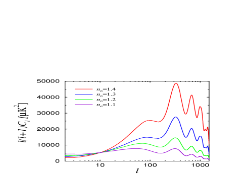
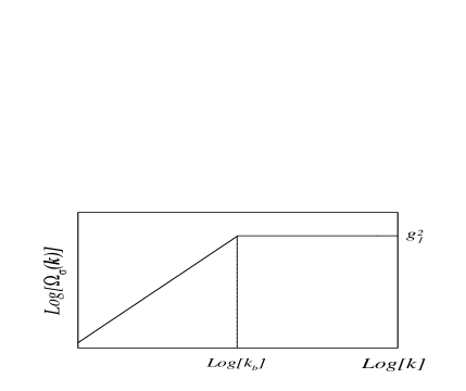
Figure 1: In the left panel, the CMB anisotropy power spectrum dependency on the primordial axion spectral index $n_{\sigma}$ is shown. We have considered a flat universe with $\Omega_{m}=0.3$ and $\Omega_{\Lambda}=0.7$ and an axionic spectral index (from top to bottom) $n_{\sigma}=1.4,~{}1.3,~{}1.2,~{}1.1$. In the right panel we show the shape of the axion spectrum.

In Fig. 1 we plot the dependence of the CMB anisotropy power spectrum on the primordial axion spectral index $n_{\sigma}$. A slightly tilted spectral index ($1.3\mathrel{\hbox to0.0pt{\lower 3.0pt\hbox{$\mathchar 536\relax$}\hss}\raise 2.0pt\hbox{$\mathchar 316\relax$}}n_{\sigma}\mathrel{\hbox to0.0pt{\lower 3.0pt\hbox{$\mathchar 536\relax$}\hss}\raise 2.0pt\hbox{$\mathchar 316\relax$}}1.4$) is required to have a sufficiently high peak. Together with the normalization condition of the axion spectrum imposed by Eq. (4), namely $\Omega_{\sigma}(k_{1})\simeq g_{1}^{2}$, this requires, in the simplest case, the presence of a kink in the spectrum. At very large scales the axion spectrum must be slightly blue, to fit the CMB data, and only at an intermediate break scale, $k_{b}$, it must become flat (see Fig. 1). This requires, in terms of the evolution of the scale factors in the pre-big bang, $\alpha\mathrel{\hbox to0.0pt{\lower 3.0pt\hbox{$\mathchar 536\relax$}\hss}\raise 2.0pt\hbox{$\mathchar 318\relax$}}-\beta$, i.e. a slower expansion of the external dimensions and, correspondingly, a somewhat faster contraction of internal dimensions at very early (negative) time.

We do not want to specify the event which may have triggered such a transition from $n_{\sigma(k<k_{b})}=1+\epsilon$ to $n_{\sigma(k>k_{b})}=1$ but it is interesting to note that isotropic expansion and contraction in a $26$-dimensional space-time gives just about the “tilt” needed to fit the observed CMB anisotropies (see below).

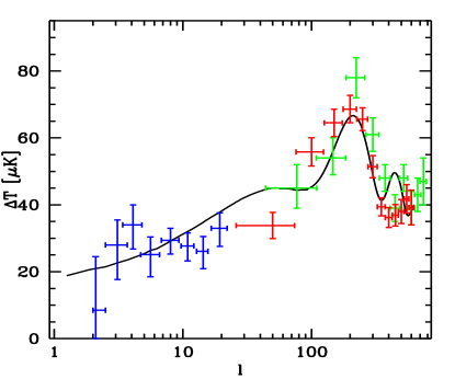
Figure 2: In the left panel, the $68\%$, $95\%$, and $99\%$ confidence levels for the cosmological parameters $\Omega_{\Lambda}$ and $\Omega_{m}$, from the peak position detected by BOOMERanG and MAXIMA-1 for the axion model (dashed). The solid contours are obtained including the SN1a data. In the right panel we compare our best fit CMB anisotropy spectrum with the COBE, MAXIMA and BOOMERanG98 data.

As shown in Fig. 1, the CMB anisotropy power spectra display two characteristic isocurvature signatures which are absent in adiabatic models. These are an isocurvature hump at $\ell\sim 40$ and the position of the first acoustic peak at $\ell\sim 300$ for a flat universe. While the presence of the hump is unavoidable, the position of the peak can be changed by a suitable choice of cosmological parameters.

In order to have a first peak at $\ell\sim 200$, we rescale our CMB anisotropy power spectrum in position, $\ell_{\rm rescaled}=\ell_{\rm flat}/R$, by the angular diameter distance parameter for a closed universe, $R=(1/2)\sqrt{\Omega_{m}/|\Omega_{K}|}\sin y$. Here $\Omega_{K}=1-\Omega_{m}-\Omega_{\Lambda}$ is the curvature parameter and $y$ is the following integral:

$$y=\sqrt{|\Omega_{K}|}\int_{0}^{z_{dec}}{dz\over[\Omega_{m}(1+z)^{3}+\Omega_{K}(1+z)^{2}+\Omega_{\Lambda}]^{1/2}}.$$ (6)

The condition $R=$ const. identifies curves in the $\Omega_{m}-\Omega_{\Lambda}$ plane, with nearly degenerate $C_{\ell}$ spectra. In Fig. 2 we plot the confidence levels in the $\Omega_{\Lambda}-\Omega_{m}$ plane which are then combined with SN1a results SN1 . It is clear that the model can be brought in reasonable agreement with observations only if the universe is moderately closed, with $\Omega_{\Lambda}\sim 0.85$ and $\Omega_{m}\sim 0.4$, which is also compatible with cluster abundance and X-ray data.

In Fig. 2 we also compare the CMB anisotropy power spectrum of our model for this choice of cosmological parameters with the COBE, MAXIMA-1, and BOOMERanG98 data. The position of the first acoustic peak has been correctly adjusted; nonetheless, the width of the peak, compressed by the increase of $R$, as well as the isocurvature hump, are still not in very good agreement with the data. The resulting normalized $\chi^{2}$ is about $\sim 1.8$ for the best-fit, which “excludes” the model at 70% confidence . Clearly more and better data around the isocurvature hump region, i.e. $\ell\sim 50$, is needed to decide definitely whether the model is ruled out.

Even if our model will turn out to disagree with better data, we believe that we learn the important lesson that cosmological parameters obtained from CMB anisotropies are strongly model dependent, a point which is swept under the carpet by the vast majority of the circulating “parameter-fitting” literature. We believe that it is very important in the future to concentrate on model independent quantities, like inter-peak distances, to determine cosmological parameters.

References

- (1) G. Veneziano, Phys. Lett. B 265 287 (1991); M. Gasperini and G. Veneziano, Astropart. Phys. 1, 317 (1993); Mod. Phys. Lett. A 8, 3701 (1993); Phys. Rev. D 50, 2519 (1994).
- (2) M. Gasperini and M. Giovannini, Phys. Lett. B 282, 36 (1991); Phys. Rev. D 47, 1519 (1993); M. Gasperini and G. Veneziano, Ref. 1 ; R. Brustein, M. Gasperini, M. Giovannini, V. F. Mukhanov and G. Veneziano, Phys. Rev. D 51, 6744 (1995).
- (3) E. J. Copeland, R. Easther and D. Wands, Phys. Rev. D 56, 874 (1997); E. J. Copeland, J. E. Lidsey and D. Wands, Nucl. Phys. B 506, 407 (1997).
- (4) R. Durrer, M. Gasperini, M. Sakellariadou and G. Veneziano, Phys. Rev. D 59, 043511 (1999).
- (5) P. de Bernardis et al., Nature 404, 955 (2000); S. Hanany et al., astro-ph/005124, Ap. J. Lett. submitted (2000).
- (6) A. Melchiorri, F. Vernizzi, R. Durrer and G. Veneziano, Phys. Rev. Lett. 83, 4464 (1999); F. Vernizzi, A. Melchiorri and R. Durrer, astro-ph/0008232, submitted to Phys. Rev. D (2000).
- (7) S. Perlmutter et al., Nature, 391, 51 (1999).