Quasar luminosity and twin effects induced by filamentary and planar structures

Abstract

We consider filamentary and planar large scale structures as possible refraction channels for electromagnetic radiation coming from cosmological structures. By this hypothesis, it is possible to explain the quasar luminosity distribution and, in particular, the presence of ”twin” and ”brother” objects. Method and details of simulation are given.

1 Introduction

Gravitational lensing (Straumann et al. 1998) is today considered a basic tool to investigate the large scale structure of the universe and to perform tests of cosmological models. Furthermore, it plays a relevant role in the dark matter search from small to large scales. On the other hand, the lensing effects can be explained by considering the action of a weak gravitational field deflecting the light rays which come from a fixed source. In other words, it is possible to define a refraction index, connected to the Newtonian gravitational field.

However, it is worthwhile to note that, in optics, there are other kinds of effects and instruments, like optical fibres and waveguides, which use the same deflection principles: The analogy with the gravitational field can be extended also to these processes taking into account a sort of ”nonlinearity” in gravitational lensing.

Considering the concept of ”channel” of sister sciences, we have refraction channels, acoustic channels and several other examples where propagating waves are trapped by some structures.

In cosmology, matter distributions, able to produce gravitational potential inducing such ”channelling effects”, could explain several anomalies which are hard to connect to standard gravitational lensing models, like, for example, the existence of objects with the same spectrum and redshift, but placed in the sky at large angular distances (e.g. twins). The huge luminosity of quasars (Fan et al. 2000; Zheng et al. 2000) could be explained by using planar cosmological structures too. In fact, taking into account expanding bubbles, produced during first order phase transition, a matter density gradient is generated when they come in touch each other. Such expanding bubbles create tridimensional spatial structures like hexahedrons (e.g. honeycombs) to minimize the interstitial space. However the growth is different with respect to crystal models since in these last cases the growth is stopped in such a direction as well as a cell of the lattice touches with an other expanding crystal in the same direction. In cosmology, we have to take into account the expansion of the universe.

Our hypothesis is that the surfaces of such hexahedrons, which are contact surfaces, could be approximated by planar structures acting as channels for electromagnetic radiation.

Furthermore, as we will discuss below, also filamentary structures could act like channels too.

In principle, all primordial topological defects as cosmic strings, textures and domain walls (Vilenkin 1984; Vilenkin 1985) could be evolved so that today they can trap electromagnetic or gravitational radiation (Capozziello & Iovane 1998; Turner et al. 1986).

This gravitational waveguiding effect has the same physical reason of the gravitational lensing effect, which account for the light deflection given by a gravitational field acting like a refraction medium . However, there are some substantial differences: the gravitational lenses are usually compact objects. On the contrary, the density can be low in these gravitational channels; moreover the radiation is deflected by the lens, but it does not pass through the object, while the light have to travel ”inside” the matter distribution in the case of gravitational channels.

The existence of a waveguiding effect could explain the huge luminosity of very far objects like quasars. Another effect could be the generation of twins and brothers. In other words, an observer could detect two images of the same object: The real image and the one catched by gravitational channel.

From a theoretical point of view, the matter distribution should locally produce an effective gravitational potential of the form $\Phi\left(r\right)\sim r^{2}$.

It is worthwhile to note that the specific form of $r$ (and then of the effective gravitational potential) depends on the particular symmetry of the situation. As we shall discuss below, we have $r=x$ for ”planar” mass distributions while $r=\sqrt{x^{2}+y^{2}}$ in the case of ”filamentary” distributions. In both cases, we are assuming an almost constant density $\rho$ which is substantially different with respect to the background.

The planar or filamentary distributions, essentially connected to a gradient of matter density, could be generated at the contact surfaces among several expanding bubbles.

The paper is organized as follows. In the Sec.2, the theoretical model for gravitational channels is developed. Sec.3 is devoted to the discussion of early cosmological phase transition, topological defects and possible connections to the today observed large scale structures. In Sec. 4, we present a simulation by which we try to explain the luminosity distribution of quasars assuming  that a part of them has been ”twined” because the radiation emitted from them have undergone a channelling process by intervening filamentary or planar large scale structures. The results are discussed in Sec.5. Conclusions are drawn in Sec.6.

2 Light propagation by gravitational refraction channels

The behaviour of the electromagnetic field, without source and in the presence of a gravitational field (Schneider, Ehlers, Falco 1992) can be described by the Maxwell equations

$$\frac{\partial F_{\alpha\beta}}{\partial x^{\gamma}}+\frac{\partial F_{\beta\gamma}}{\partial x^{\alpha}}+\frac{\partial F_{\gamma\alpha}}{\partial x^{\beta}}=0;\quad\frac{1}{\sqrt{-g}}\frac{\partial}{\partial x^{\beta}}\left(\sqrt{-g}F^{\alpha\beta}\right)=0,$$ (1)

where $F^{\alpha\beta}$ is the electromagnetic field tensor and $\sqrt{-g}$ is the determinant of the four–dimensional metric tensor. For a static gravitational field, these equations can be reduced to the usual Maxwell equations describing the electromagnetic field in media where the dielectric and magnetic tensor permeabilities are connected to the metric tensor $g_{\mu\nu}$ by the equation

$$\varepsilon_{ik}=\mu_{ik}=-g_{00}^{-1/2}[\mbox{det}g_{ik}]^{-1/2}g_{ik}\quad i,k=1,2,3.$$ (2)

If  the medium is isotropic, the metric tensor is diagonal and the refraction index is $n\left(r\right)=\left(\varepsilon\mu\right)^{\frac{1}{2}}$ (Capozziello & Iovane 1999).

In the weak field approximation, the metric tensor components are (Blioh & Minakov 1989; Landau & Lifsits 1975)

$$g_{00}\simeq 1+2\frac{\Phi(\mathbf{r})}{c^{2}}\;;\qquad g_{ik}\simeq-\delta_{ik}\left(1-2\frac{\Phi(\mathbf{r})}{c^{2}}\right)\;,$$ (3)

where, $\Phi(\mathbf{r})$ is the Newtonian  potential and we are assuming the weak field, $\Phi/c^{2}\ll 1$, and the slow motion approximation $|v|\ll c$.

Channeling solutions can be obtained, by reducing Maxwell equations in a medium to the scalar Helmoltz equation for the fields $\mathbf{E}$ and $\mathbf{H}$ . For the electrical field, after Fourier transformation, we can write (Capozziello & Iovane 1998)

$$\triangle\mbox{\bf E}_{\omega}(\mbox{\bf r})+\frac{\omega^{2}}{c^{2}}n^{2}(\omega,\mbox{\bf r})\mbox{\bf E}_{\omega}(\mbox{\bf r})=0\,$$ (4)

where $\omega$ is the frequency of the given Fourier component.

A similar equation holds for the magnetic field. The general solution has the form

$$\mbox{\bf E}_{\omega}(\mbox{\bf r})=\mbox{\bf E}_{\omega}^{(0)}(\mbox{\bf r})+\int\mathcal{G}({\bf\tilde{r}},{\bf r}^{\prime},\omega)\nabla\left[\frac{{\bf E}_{\omega}^{(0)}({\bf\tilde{r}})\nabla\varepsilon(\omega,{\bf\tilde{r}})}{\varepsilon(\omega,{\bf\tilde{r}})}\right]d{\bf\tilde{r}},$$ (5)

where $\mathcal{G}$ is the Green function for the equation

$$\left[\triangle+\frac{\omega^{2}}{c^{2}}n^{2}(\omega,\mbox{\bf r})\right]\mathcal{G}(\mbox{\bf r},\mbox{\bf r}^{\prime},\omega)=\delta(\mbox{\bf r}-\mbox{\bf r}^{\prime})\,.$$ (6)

This is a Schrödinger-like equation for the energy constant $E=0$. In fact, if we write down the Hamiltonian operator $\hat{\mathcal{H}}=-\frac{1}{2}\triangle+U(\mbox{\bf r})\,,$with $\hbar=m=1$ and ${\displaystyle U({\bf r})=-2\frac{\omega^{2}}{c^{2}}n^{2}(\omega,{\bf r})\,},$ a fully analogy between the two problems is obtained. $U(\mbox{\bf r})$ assumes the role of the Newtonian potential $\Phi(\mathbf{r})$.

Let us consider the scalar Helmoltz equation for an arbitrary monochromatic component of the electric field

$$\frac{\partial^{2}E}{\partial z^{2}}+\frac{\partial^{2}E}{\partial x^{2}}+\frac{\partial^{2}E}{\partial y^{2}}+k^{2}n^{2}(\mathbf{r})E=0\,,$$ (7)

where $k$ is the wavenumber. The coordinate $z$ can be considered as the longitudinal one and it can measure the space distance along the structure produced by a mass distribution with an optical axis.

Let us consider now a solution of the form

$$E=n_{0}^{-1/2}\Psi\exp\left(ik\int^{z}n_{0}(z^{\prime})dz^{\prime}\right)\;;\quad n_{0}\equiv n(0,0,z)\,,$$ (8)

where $\Psi(x,y,z)$ is a slowly varying spatial amplitude along the $z$ axis, and $\exp(iknz)$ is a rapidly oscillating phase factor. Its clear that the beam propagation is along the $z$ axis. We rewrite the Helmoltz equation neglecting the second order derivative in longitudinal coordinate $z$ and obtain a Schrödinger–like equation for $\Psi$:

$$i\lambda\frac{\partial\Psi}{\partial\xi}=$$

$$=-\frac{\lambda^{2}}{2}\left(\frac{\partial^{2}\Psi}{\partial x^{2}}+\frac{\partial^{2}\Psi}{\partial y^{2}}\right)+\frac{1}{2}\left[n_{0}^{2}(z)-n^{2}(x,y,z)\right]\Psi,$$ (9)

where $\lambda$ is the electromagnetic radiation wavelength and we adopt the new variable ${\displaystyle\xi=\int^{z}\frac{dz^{\prime}}{n_{0}(z^{\prime})}\,}$ is a new normalized variable with respect to the refraction index. It is interesting to stress that the role of Planck constant is assumed by $\lambda$.

At this point, it is worthwhile to note that if one has the distribution of matter in the form of a cylinder or a sphere with a constant (dust) density, the gravitational potential inside has a parabolic profile providing channelling effects for electromagnetic radiation analogous to the sel-foc optical waveguides realized for optical fibres. In this case, Schrödinger-like equation is a two-dimensional quantum harmonic oscillator which solutions provs the form of Gauss-Hermite polynomials (see, for example (Man’ko 1986)).

The channeling effect depends explicitly on the shape of the potential: The radiation from a remote source does not attenuate if $U\sim r^{2}$; this situation is realized supposing a ”planar” mass distribution ($r=x$) or a filamentary distribution ($r=\sqrt{x^{2}+y^{2}}$) with constant density . In other words, if the radiation, travelling from some source, undergoes a channelling effect, it does not attenuate like $1/R^{2}$ as usual, but it is, in some sense conserved; this fact means that the source brightness will turn out to be much stronger than the brightness of analogous objects located at the same distance (i.e. at the same redshift Z) and the apparent energy released by the source will be anomalously large.

To fix the ideas, let us estimate how the electric field propagates into an ideal filament whose internal potential is

$$U(r)=\frac{1}{2}\omega^{2}r^{2}\,,\;\;\;\;\;\;\omega^{2}=\frac{4\pi G\rho}{c^{2}}.$$ (10)

A spherical wave from a source has the form

$$E=(1/R)\exp(ikR)\,.$$ (11)

In the paraxial approximation, Eq. (11) becomes

$$E(z,r)=\frac{1}{z}\exp\left(ikz+\frac{ikr^{2}}{2z}-\frac{r^{2}}{2z^{2}}\right)\,,$$ (12)

where we are using the expansion

$$R=\left(z^{2}+r^{2}\right)^{1/2}\approx z\left(1+\frac{r^{2}}{2z^{2}}\right),\;\;r\ll z\,.$$ (13)

It is realistic to assume $n_{0}\simeq 1$ so that $\xi=z$.

Let us consider now that the starting point of the gravitational channel of length $L$ is at a distance $l$ from a source shifted by a distance $a$ from the structure longitudinal axis in the x direction. The amplitude of the field $E$, entering the channel, is

$$\Psi_{in}=\frac{1}{l}\exp\left[\frac{ikl-1}{2l^{2}}\left((x-a)^{2}+y^{2}\right)\right]\,,$$ (14)

so that we have $R=\left(l^{2}+y^{2}+(x-a)^{2}\right)^{1/2}.$ We can calculate the amplitude of the field at the exit of the filament by the equation

$$\Psi_{out} (x,y,l+L)=$$ (15)

$$=\int dx_{1}dy_{1}\mathcal{G}(x,y,l+L,x_{1},y_{1},l)\Psi_{in}(x_{1},y_{1},l),$$

where $\mathcal{G}$ is again the Green function for $\Psi$. In particular, taking into account the potential (10), $\mathcal{G}$ is the propagator of the harmonic oscillator; then $\Psi_{out}$ is a Gaussian integral that can be exactly evaluated. There are two interesting limit for $\Psi_{out}$.

If $\omega l\ll 1$, we have

$$\Psi_{out}=\frac{1}{i\lambda}\exp\left\{-\frac{l+i\lambda}{2\lambda^{2}l}\left[(x+a)^{2}+y^{2}\right]\right\}\,,$$ (16)

which means that the radiation emerging from a point with coordinate $(a,0,0)$ is focused near a point with coordinates $(-a,0,l+L)$ (that is the radius has to be of the order of the wavelength). This means that, when the beam from an extended source is focused inside a gravitational channel at a distance $L$, an inverted image of the source is formed, having the very same geometrical dimensions of the source. The channel ”draws” the source closer to the observer since, if the true distance of the observer from the source is $R$, its image brightness will correspond to that of a similar source at the closer distance

$$R_{eff}=R-l-L\,.$$ (17)

In the opposite limit, $\omega l\gg 1$, we have $\tan\omega L\rightarrow\infty$, so that $L\simeq\pi/\omega$, that is the shortest focal length of the gravitational channel is

$$L_{foc}=\sqrt{\frac{\pi c^{2}}{4G\rho}}\,.$$ (18)

It is relevant to note that the expression  $L_{foc}$ leads to  values of about 100 Mpc for a typical galactic density $\rho_{0}\sim 10^{-24}\,g/cm^{3}$. In other words, this can be assumed as a typical length for large scale structures.

3 Are there candidates for cosmological refraction channels?

Early structures, resulting from inflationary phase transitions, could be good candidates to implement the above filamentary or planar structures acting as cosmological refraction channels. Essentially, if the primordial universe undergoes a first or second order phase transition, such a transition takes place on a short time scale ( $\tau<H^{-1}$ ), and it will lead to correlation regions inside of which the value of a certain scalar field $\varphi$ (the inflaton which leads dynamics) is approximately constant, but outside $\varphi$ ranges randomly over the vacuum manifold. In the simplest case, for a Ginzburg-Landau-like potential of the form

$$V\left(\varphi\right)=\frac{\lambda}{4}\left(\varphi^{2}-\varphi_{0}^{2}\right)^{2},$$ (19)

the correlation regions are separated by domain walls, regions in space where $\varphi$ leaves the vacuum manifold $\mathcal{M}$ and where, therefore, potential energy is localized. This energy density can act as a seed for structure.

There are various types of local and global topological defects (Kibble 1976) (regions of trapped energy density) depending on the number of real components of $\varphi$ (being, in general, $\varphi^{2}=\sum\nolimits_{i=1}^{n}\varphi_{i}^{2}$). In the case of domain walls $n=1$.

The rigorous mathematical definition refers to the homotopy of $\mathcal{M}$ . The words ”local” and ”global” refer to whether the symmetry, which is broken, is a gauge or global symmetry. In the case of local symmetries, the topological defects have a well defined core outside of which $\varphi$ contains no energy density in spite of non vanishing gradients $\nabla\varphi$ ; the gauge field can absorb the gradient, i.e. $D_{\mu}\varphi=0$  when $\partial_{\mu}\varphi\neq 0$. Global topological defects, however, have long range density fields and forces.

Practically, the topological defects can be classified by their topological characteristic which, in term of the scalar field $\varphi$ , depends on the number of real components.

Pointlike defects ($n=3$) give monopoles, linear defects ($n=2$) give cosmic strings, surfaces-like defects ($n=1$) are domain walls, hypersurface-like defects, but not properly topological defects, with $n=4$, are textures.

In principle, all these structures can be seeds for large scale structures depending on the cosmological model we adopt. Taking into account realistic scenarios, the best candidates seem to be cosmic strings.

Furthermore, any first-order phase transition proceeds via bubble nucleation so that invoking filamentary and planar structures for channeling effects is reasonable (local surface portions of large bubbles can be approximated to planar structures).

For example, cosmic strings easily realize the condition to obtain a Newtonian potential useful, as discussed above, to produce a gravitational refraction channel. In fact, in the weak energy limit approximation, these topological defects are described internally by the Poisson equation $\nabla^{2}\Phi=\rho_{0}$ and externally by $\nabla^{2}\Phi=0$ , where $\rho_{0}$ is a constant. The condition on the density gradient is naturally recovered. Another useful feature is that they act as gravitational lenses after the quasar formation (Vilenkin 1985; Gott III 1985) Immediately we get, internally, $\Phi\sim r^{2}\$and, by the dynamical evolution of the universe, strings can evolve into structures with lengths of the order $\ \sim 100$ Mpc. However, also after evolution, strings remain ”wires” and then, in order to get the cylindrical structures which we need for gravitational channels (e.g. a filament of galaxies), we have to invoke further processes where strings are seeds to cluster matter at large scales.

Furthermore, the motion of cosmic strings with respect to the background produces wakes and filaments which are able to evolve into large scale structures like clusters or filaments of galaxies (Vachaspati & Vilenkin 1991).

All these arguments, as it is well known, are hypotheses for large scale structure formation.

Our issue is now to construct reasonable toy models which, by channeling effects, could explain, in a simple way, the huge luminosity of quasars and twin effects in gravitational lensing.

4 The model

The major aim of our simulation is to perform a test about the possibility that twin or brother quasars could be explained by trapped and guided light, which was emitted by quasar sources and guided thanks to structures acting like channels. Moreover, the single quasar itself could be a typical object (a bulge of a standard galaxy) which appears so magnified thanks to the presence of channelling effects.

In our simulation, as discussed above, we can take into account a gravitational first order phase transition from which false vacuum bubbles nucleate inside a true vacuum cosmological background. Our fundamental assumption is that they cosmologically evolve giving rise to a cellular structure capable of yielding the observed large scale structures (Kolb & Turner 1990). After, we take into account also filamentary large scale structures.

It is also important to note that, due to the cosmological expansion, the bubbles continue to grow even after they collide; this is the difference with models used in crystal growth such as the Voronoi and the Johnson-Mehl models, where crystals stop to grow in the direction of the neighbour one.

By simple geometric arguments, we can put around a circle other six circles in a given area, with the same radius. If these circles are expanding, to minimize the space among them, they degenerate into hexagons. The Fig. 1 shows the situation.

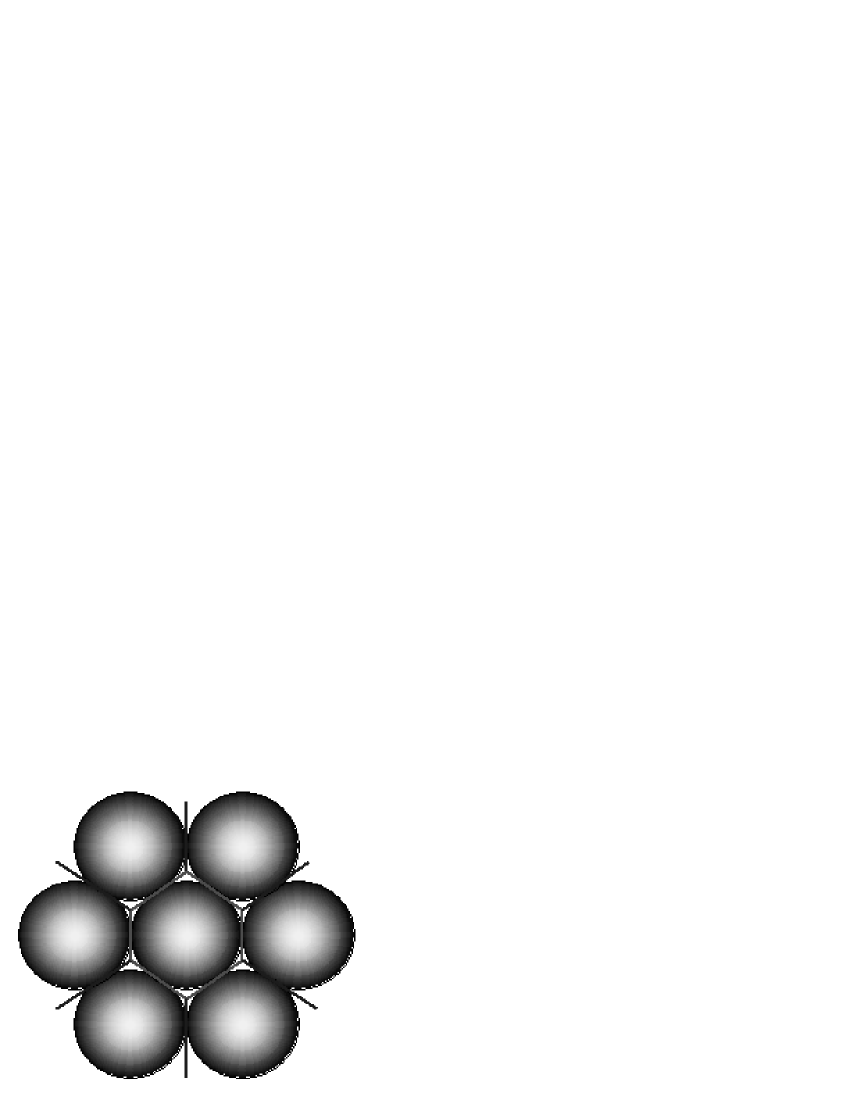
Figure 1: Model for the formation of contacting planar structures.

In other words, density gradients of matter will be generated among the hexagons in the boundary regions. In three dimension, the spheres will degenerate into dodecahedrons by forming a typical honeycomb structure with 2-dimensional elementary pentagonal cells (see Fig. 2), whose surfaces will give rise to planar structures with matter density different from zero.

Finally, given an expanding universe several dodecahedrons, remnants of a primordial gravitational phase transition, could yield a sort of honeycomb structure. The isotropy and homogeneity would be preserved at larger scales (size $\sim 1000$ Mpc).

In this case, the formation of clustered galactic structures will be naturally due to the contact among several spheres, which would give rise to density gradients.

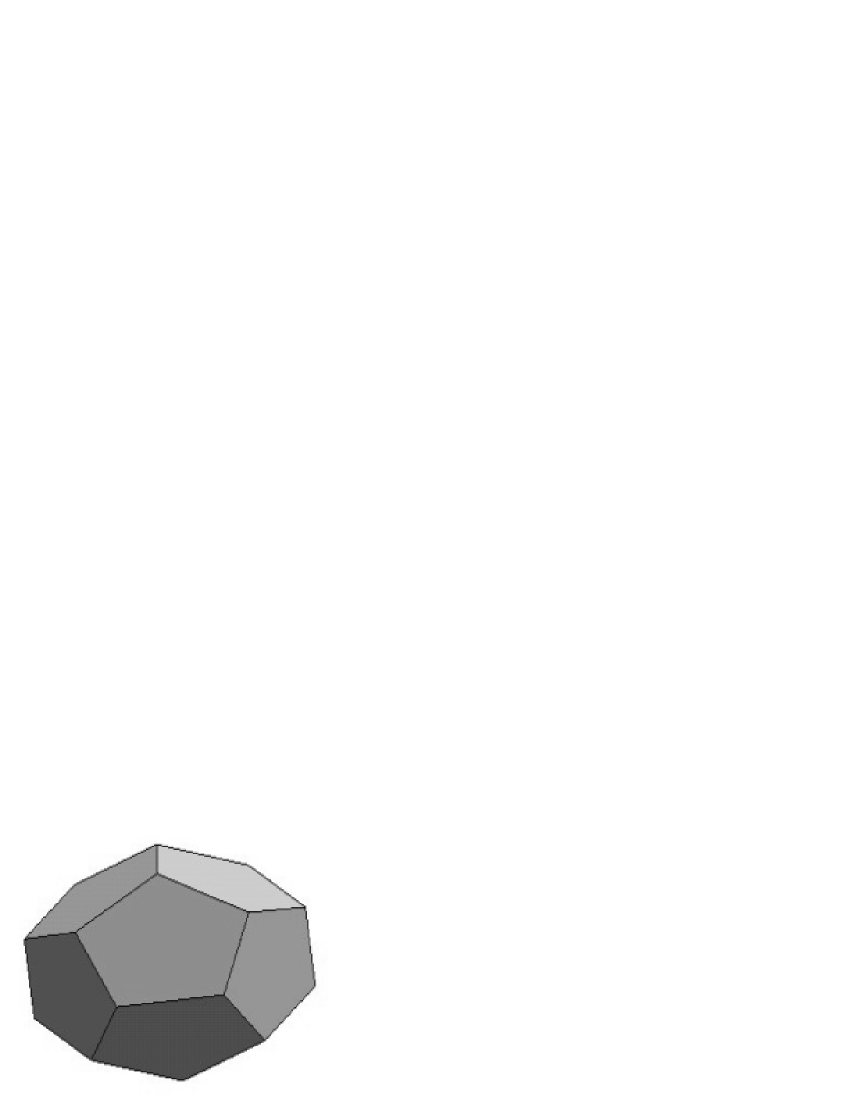
Figure 2: Elementary cell like dodecaedron.

Such planar structures on contact surfaces could act as refraction channels, e.g. they could trap and guide the light due to the quasi-constant surface density; in this way, we should see a universe like that observed. To be more precise, we do not see an exact honeycomb, but a selfsimilar structure (Sylos Labini, Mountuori & Pietronero 1998) like those described in fractal models: in a more realistic model, we have to consider several spheres with different radii $R_{i}$ (we have not a perfect dodecahedron, but a more complicate polyhedron, see for example, Fig. 3). Dynamics will be governed by the symmetry breaking during the phase transition: vacuum density could be different in different bubbles. However, we can obtain relevant results just taking into account balls with the same radius, that is, by considering bubble nucleation at same density and expanding rate at constant speed $v$. Similar considerations can be done also for filamentary structures which act as refraction channels.

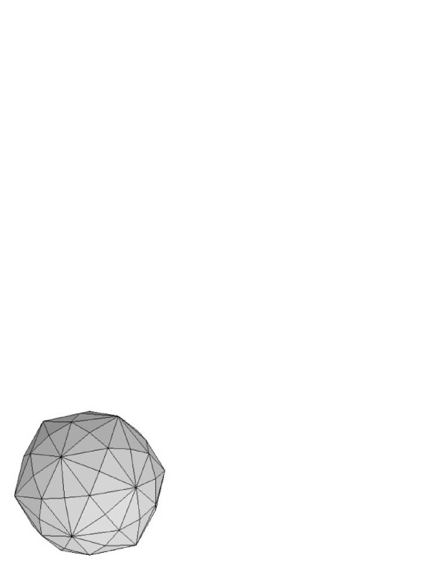
Figure 3: Elementary cell like trapezoidal icositetrahedron.

4.1 Hypotheses and previsions of the simulation

Let us consider a universe model with an observed radius $R_{0}=3000$ Mpc. Furthermore, let us assume $10^{4}$ quasars uniformly and isotropically distributed in this spherical space. The positions of the objects are fixed in a random way by using a random number generator. Moreover, the quasars are point-like objects. Furthermore, it is supposed that every single quasar emits light in an isotropic way.

Between the refraction channels, we have to distinguish filamentary structures and planar structures.

We produce randomly distributed filamentary structures with a dimension of about 100 Mpc along the major axis and a shape like a cylinder with 5 points, where the longitudinal axis of the cylinder changes its direction. A typical simulated channel is shown in the Fig. 4.

In particular, the channels of the model are built by five cylinders with a length of $1\div 20$ Mpc and radius $r\sim 1\div 100$ Kpc. The positions of the channel starting points, that is the centres of the first base circle in the first cylinder and the longitudinal axis of the cylinder are randomly generated.

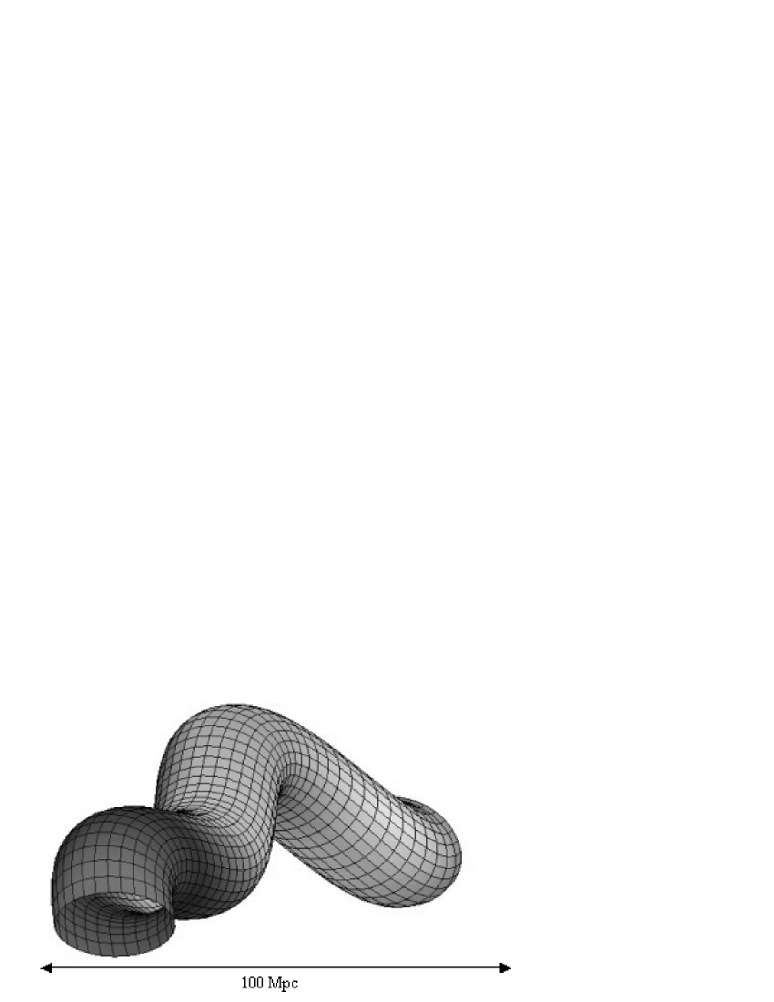
Figure 4: A typical simulated channel.

There is a constraint on this generation: we assume that the cylinders cannot collapse in a compact object. In other words, by defining $\theta_{i}$ and $\phi_{i}$ the angles in the links between two consecutive cylinders along their longitudinal axis (see Fig. 5), we impose:

$$0<\vartheta_{i}<\pi/2\qquad and\qquad 0<\varphi_{i}<2\pi,$$

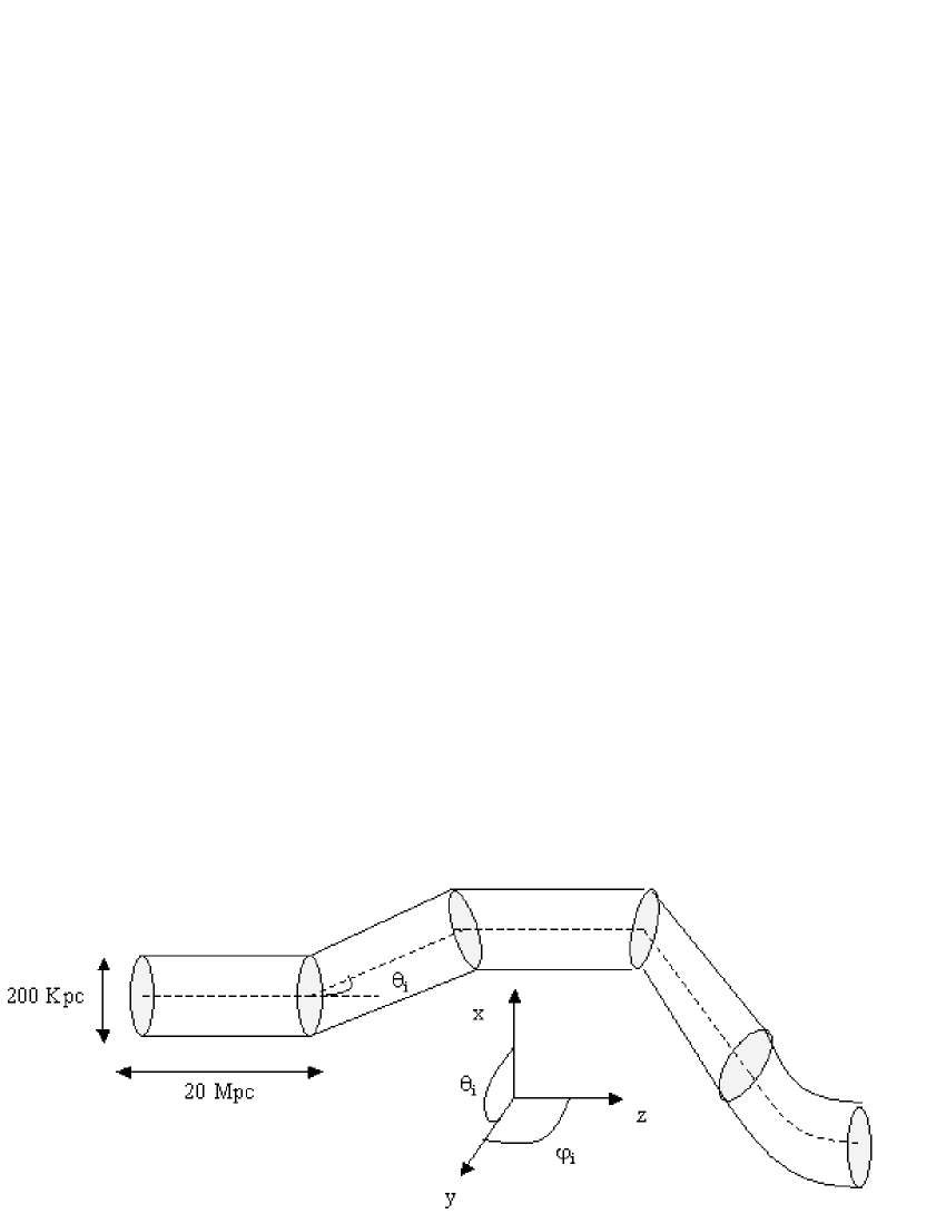
Figure 5: Scheme of a channel.

with $\vartheta_{i}$ and $\varphi_{i}$ randomly selected.

Alternatively, we can have casually distributed planar structures acting like refraction channels, with linear dimensions of about $100$ Mpc, on pentagonal surfaces.

In particular, in a universe with a radius $R_{0}=3000$ Mpc, we can inscribe several pseudo-balls $b_{i}$ with a radius $R_{i}$ such that the linear dimensions have an extension of about $l_{i}=100$ Mpc. This can be made in different ways:

1) Let us consider a circular sector with an angular spread of $\pi/24=7.5{{}^{\circ}}$; by assuming that the linear extension of the structure is of 100 Mpc, we obtain:

$$100\ \text{Mpc}=l_{i}=\frac{\pi}{24}R_{i}\quad\rightarrow\quad R_{i}=764\ \text{Mpc.}$$ (20)

In this case, we can inscribe $n_{balls}=60$ balls with a radius $R_{i}$ in the universe with a radius $R_{0}$. Moreover, we have to calculate the error by assuming

$$2\pi R_{i}=4800\ \text{Mpc},\ l=100\ \text{Mpc}\quad\rightarrow\quad\epsilon=\frac{l}{2\pi R_{i}}=2\%.$$

2) By assuming a circular sector with an angular spread of $\pi/18=10{{}^{\circ}}$, we obtain

$$R_{i}=573\ \text{Mpc},\quad n_{balls}=143,\quad\epsilon=3\%.$$

3) By assuming a circular sector with an angular spread of $\pi/12=15{{}^{\circ}}$, we obtain

$$R_{i}=382\ \text{Mpc},\quad n_{balls}=484,\quad\epsilon=4\%.$$

4) By assuming a circular sector with an angular spread of $\pi/10=18{{}^{\circ}}$, we obtain

$$R_{i}=318\ \text{Mpc},\quad n_{balls}=840,\quad\epsilon=5\%.$$

5) Finally assuming a circular sector with an angular spread of $\pi/9=20{{}^{\circ}}$, we obtain

$$R_{i}=286\ \text{Mpc},\quad n_{balls}=1154,\quad\epsilon=6\%.$$

In the simulation, it is useful to implement an attenuation mechanism to make the model more realistic. If the sources are at distances of the order of $1000$ Mpc, since the luminosity decreases as $R^{-2},$ we assume that only fluxes large enough to survive to this physical cut can be detected as the channelling effects intervene. Otherwise they are completely absorbed by intergalactic media.

Next step is to verify how much light is trapped by the intervening channels and how many sources are lensed and then appear as twin images to the observer.

4.2 The implementation

The simulation is made by using the New Object Visual Programming Technique (National Instruments: Reference Manual 1998; National Instruments: Functions Manual 1998; National Instruments: G-Math Manual 1998).

The simulation is built up by a main program, that calls and manages a collection of subprocesses described as follows.

1) The first process is built up by 5 secondary sequences:

1.1) The first one - sequence 1.1 - gives the quasar coordinates which are randomly generate;

1.2) The second one - sequence 1.2 - gives the photons coming out from quasars: in this step the arrival points of coming out photons are evaluated;

1.3) The third one - sequence 1.3 - generates the light rays at each quasar position;

1.4) The fourth one - sequence 1.4 - rejects all photons out of $2R_{0}=6000$ Mpc (the boundary of our toy universe);

1.5) The fifth one - sequence 1.5 - prepares a multidimensional array and a file to perform and to save the intersections between the rays and the waveguides;

2) The second process regards the objects, whose light is picked up, trapped and guided by the structures (it gives the twined quasars);

3) The third process has two sequences:

3.1) generates the refraction channel in random positions into the spherical volume representing the universe;

3.2) evaluates the parameters to intersect the rays from the quasars (this subprocess is completely equivalent to 1.5);

4) The fourth process evaluates the attenuation function for the light coming from quasars;

5) The fifth process prepares the trapping;

6) The sixth process performs the trapping and guiding of light in the channels;

7) The seventh process tests that the same light rays is not counted more than one time, if it intersects more sub-cylinders of the same channel.

In Fig. 6, there are shown several examples of simulated refraction channels.

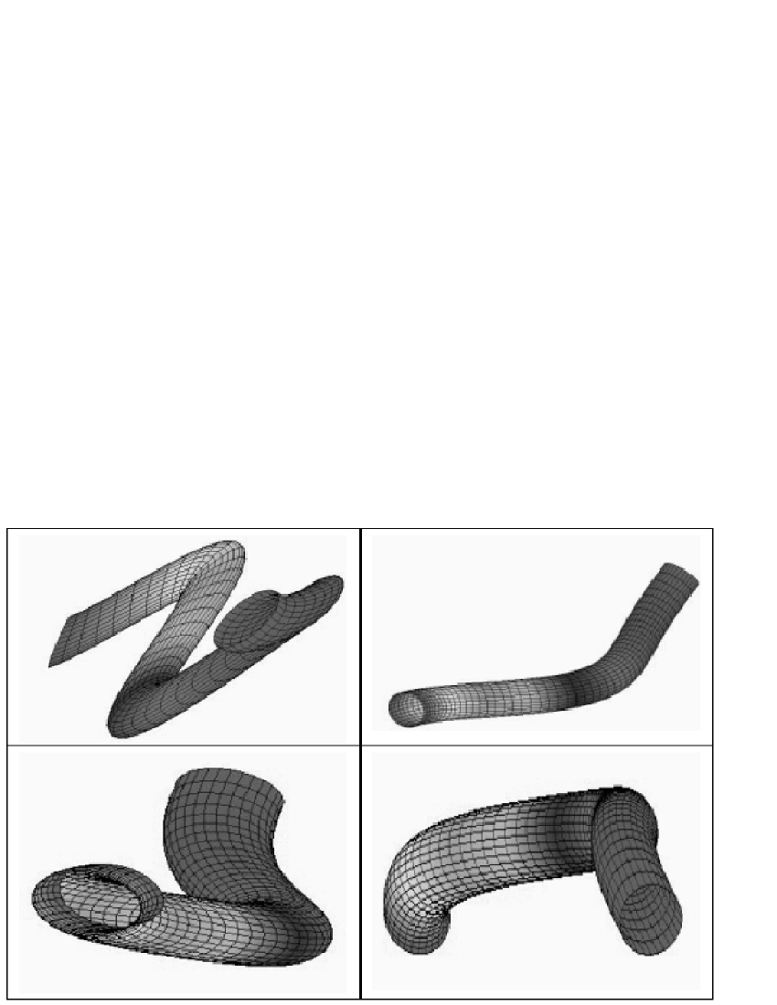
Figure 6: Some examples of simulated refraction channels.

5 The results

The results of the simulation are summarized, by considering: 1) a fixed number of channels chosen in relation to $R_{i}$ for the planar case and 200 for the filamentary one; 2) $10^{4}$ quasars randomly fixed as input.

a) The quasar positions $R$ (in Mpc) and the redshifts $Z,$ after the attenuation, have a Gaussian distribution fit with the mean value and the standard deviation in full agreement with theoretical and observative results (Capozziello & Iovane 1999; Fort & Mellier 1994; Broadhurst, Taylor, Peakock 1995);

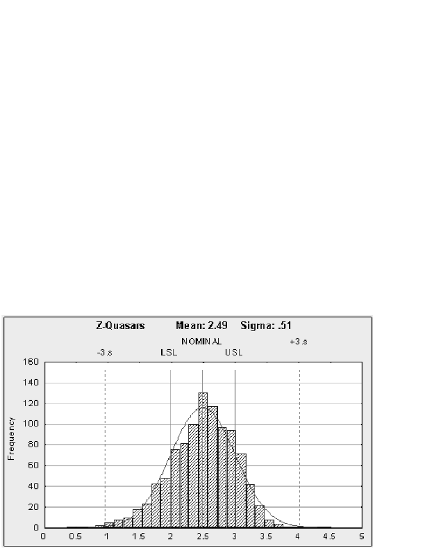
Figure 7: Quasar redshift $Z$ after attenuation process.

b) Also for the twined quasars, $R$ and $Z$ are comparable with the theoretical models; in particular, the twined quasars are a subset of the input quasars and they are also isotropically distributed in the planes $x-y$ and $x-z$.

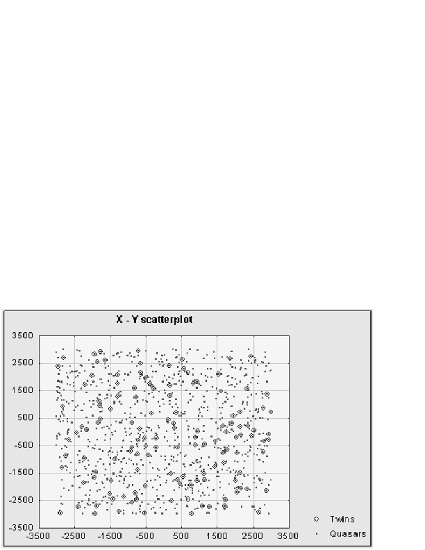
Figure 8: Scatter plot $x-y$ plane of quasars after attenuation and twined quasars.

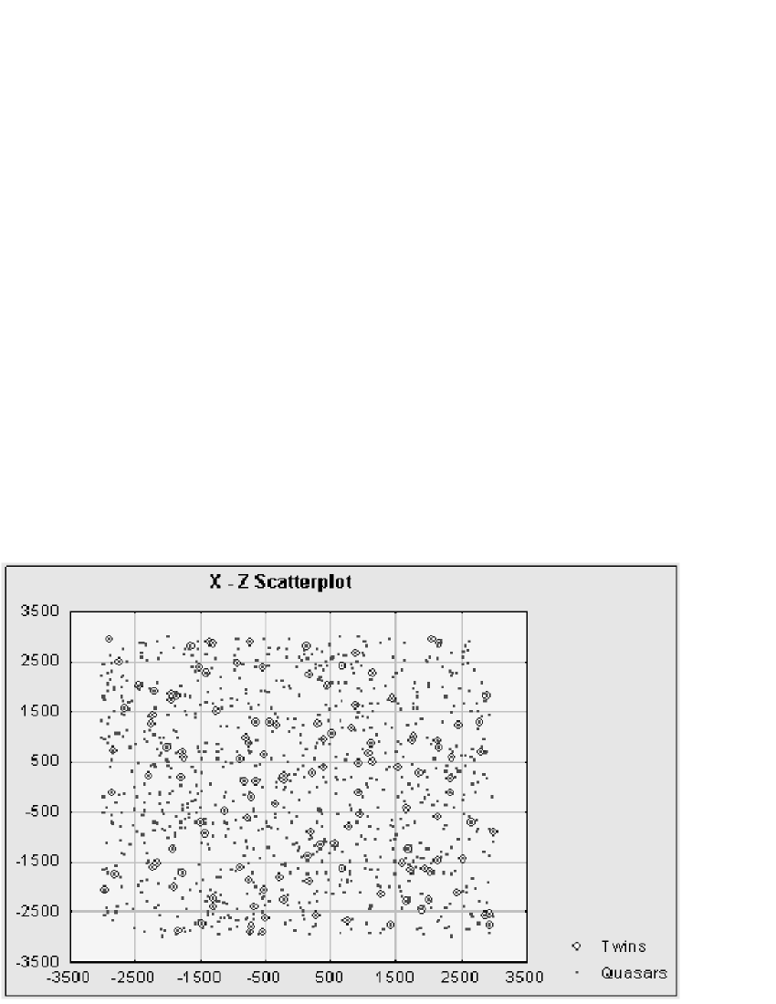
Figure 9: Scatter plot $x-z$ plane of quasars after attenuation and twined quasars.

c) The Table 1 summarizes the obtained results for the planar channels from a numerical point of view.

Input number of quasars	number of channels	number of quasars	Twined quasars	Twined Q./Q. after atten.
$10^{4}$	60	1015	109	7%
$10^{4}$	143	977	141	14%
$10^{4}$	484	995	260	26%
$10^{4}$	840	1023	337	33%
$10^{4}$	1154	981	461	35%

Table 1: Tab. 1. Simulation summary.

About 10% of initial quasars pass trough the attenuation process. A fraction, from 7% to 35% of quasars after the attenuation, undergoes a channelling effect. This fraction is linked to the number of channels. The number of twined quasars increases as the number of channels increases, by fixing the number of quasars after the attenuation. A preliminary fit can be made between the number of refraction channels and the twined quasars. Fig. 10 shows a linear correlation.

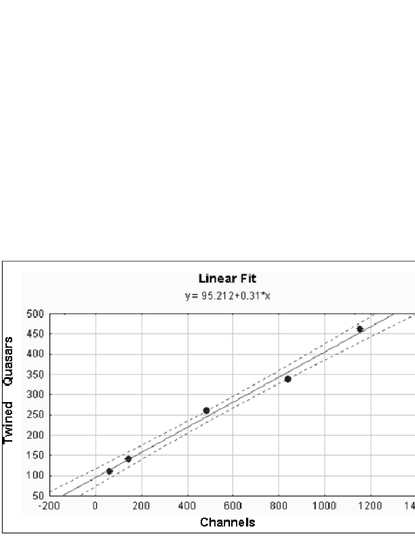
Figure 10: Linear fit between the number of channels and twined quasars.

The results are in full agreement with the filamentary channels. In fact, in this case, we have 982 quasars after the attenuation and, among them, 137 are twined. In other words, about 10% of the initial quasars pass trough the attenuation process and a fraction of about 14% of these ones undergoes a channeling effect.

In a first approximation, a superposition of the two distributions ( not twined quasars after attenuation and twined quasars) leads our analysis in the same direction of the raw theoretical model, that is, we get a Poisson-like distribution for all quasars. On the other hand, a finest analysis shows two peaks in the quasars distribution: the highest is due to non-twined quasars, whose light is not trapped and guided in the channels and the shortest is due to twined quasars . This fraction is in the range 7%-35%.

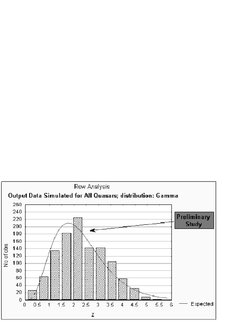
Figure 11: Expected Poisson shape in $Z$ quasars distribution like in raw theoretical models.

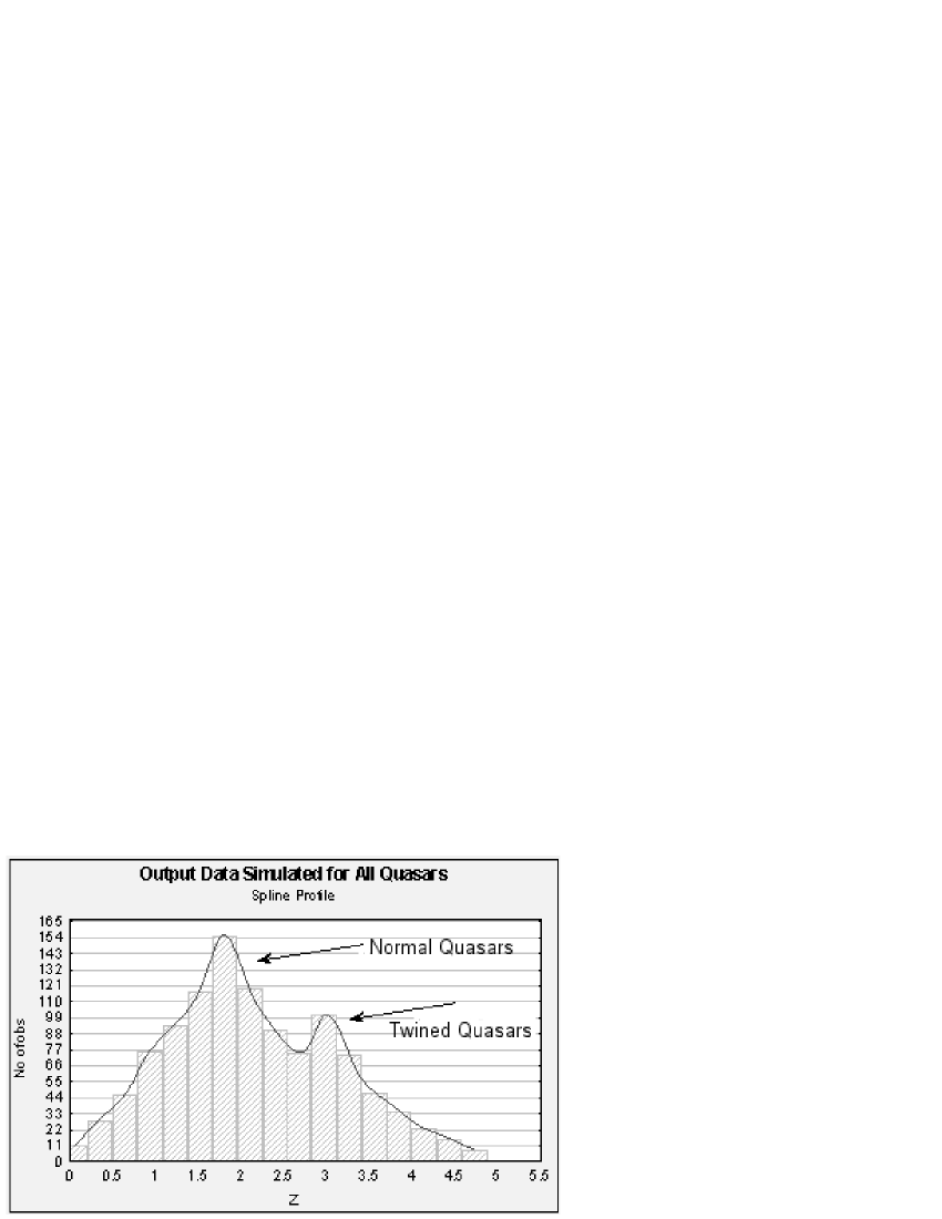
Figure 12: Double peak in quasar distribution like in observations (CRONARIO 1998).

6 Discussion and conclusion

In this paper, we propose a mechanism by which it is possible to explain two of major puzzles of quasar theory: the huge luminosity and the twin (or brother) objects. Both of them, till now, have invoked exotic explanations as the presence of a supermassive black hole inside the core radius or lensing effects, where the position and the size of intervening deflector (usually a galaxy) has to be in same sense ”fine tuned”. By our cosmological refraction channeling effects both the issues are addressed in a natural way.

The huge luminosity at far red-shift is nothing else but the effect of the channel which ”draws” the luminosity of the source closer to the observer. In this sense, quasars could be just primordial (in same sense ”ordinary”) galaxies whose luminosity in not dispersed as $1/R^{2}$ This fact means that the source brightness will turn out to be much stronger than the brightness of analogous objects located at the same distance (i.e. at the same redshift Z) and the apparent energy released by the source seems anomalously large. Besides, the large angular distance separation of twins and brothers is due to the geometry of (filamentary or planar) channels without posing ”ad hoc” lens galaxies between the source and the observer. This hypothesis, as shown, naturally explain the double peak luminosity function of quasars.

However, what we have discussed here is nothing else but a toy model. In fact, the discrete nature of matter distribution within the channels affect the light propagation (we have to take into account scattering points, dissipation, absorbtion, and dispersion in a more realistic model).

Depending on the distribution of discrete matter, we could have several places where the light could lake out.

Furthermore, the distribution of our filamentary and planar structures has to be compared to the microwave background in order to preserve the overall homogeneity and isotropy of observed very large scale structure.

All these issues deserve further studies and the comparison to the observational data.

- (1) Blioh P.V. & Mankov A.A., 1989, Gravitational Lenses, Kiev, Naukova Dumka in Russian
- (2) Broadhurst T.J., Taylor A.N., and Peakock J.A., 1995, ApJ 438 49
- (3) Capozziello S. & Iovane G., 1998, Proc. Dark98 - Heidelberg, Ed. World Scientific
- (4) Capozziello S. & Iovane G, 1999, G&C Vol.5, No.1, 17
- (5) CRONARIO Coll., 1998, Internal Communication
- (6) Fan X., White R.L., Davis M. et al., astro-ph/0005414
- (7) Fort B. & Mellier Y., 1994, A&A 5, 239
- (8) National Instruments, 1998, Labview 5.0: Refernce Manual
- (9) National Instruments, 1998, Labview 5.0: Functions Manual
- (10) National Instruments, 1998, Labview 5.0: G-Math Manual
- (11) Gott III J.R., 1985, ApJ 288 422
- (12) Kibble T.W.B., 1976, J. Phys. A9, 1387
- (13) Kolb E.W. & Turner M., 1990, Early Universe, Ed. Addison-Wesley, N.Y.
- (14) Landau L.D. & Lifsits E.M., 1975, The classical theory of fields, Ed. Pergamon Press, N.Y.
- (15) Man’ko V.I., 1986, in Lee Methods in Optics, lecture Notes in Physics, Ed. Mondragon and Wolf, 250 193
- (16) Schneider P., Ehlers J., Falco E.E.,1992, Gravitational lenses. Springer-Verlag, Berlin
- (17) Straumann N., Jetzer P., Kaplan J. 1998, Topics on gravitational lensing. Ed. Bibliopolis, Napoli.
- (18) Sylos Labini F., Montuori M., Pietronero L., 1998, Phys.Rep 293, 61
- (19) Turner E.L., Schneider D.P., Burke B.F., et al. 1986, Nature 321, 142
- (20) Vachaspati T. & Vilenkin A., 1991, Phys.Rev.Lett. 67, 1057
- (21) Vilenkin A., 1984, ApJ 282, L51
- (22) Vilenkin A., 1985, Phys. Rep 121, 263
- (23) Zheng W., Tsvetanov Z.I., Schneider D.P., et al. astro-ph/0005247