Automatic Shell Detection in CGPS Data

Abstract

A numerical code aiming at the automatic detection of spherical expanding HI shells in radio data-cubes is presented. The following five shell parameters are allowed to vary within a specified range: angular radius, expansion velocity and three center coordinates (galactic coordinates $l$ and $b$, and systemic radial velocity $V$). We discuss several factors which can reduce the sensitivity of the shell detection: the presence of noise (both instrumental and “structural”), the fragmentation and asphericity of the shell and the inhomogeneity of the background and/or foreground emission. The code is tested on four objects: two HII regions and two early B stars. We use HI data from the Canadian Galactic Plane Survey. In all four cases the evidence for an expanding HI shell is found.

Département de Physique and Observatoire du Mont Mégantic, Université de Montréal, C.P. 6128, Succursale Centre Ville, Montréal, H3C 3J7, QC, Canada

1. Introduction

Shells are omnipresent in the interstellar medium (ISM) of spiral and dwarf irregular galaxies. In some systems most of the ISM can be described as an ensemble of interacting shells and supershells (Staveley-Smith et al. 1997; Mashchenko, Thilker, & Braun 1999, hereafter MTB).

Theoretically, many astrophysical phenomena may lead to the formation of expanding HI shells: stellar winds (Weaver et al. 1977), supernova explosions (Cox 1972), the combined action of multiple supernovae and stellar winds in OB associations (Bruhweiler et al. 1980), radiation pressure from the field stars (Elmegreen & Chiang 1982) and the infall of high-velocity clouds onto the galactic plane (Tenorio-Tagle 1981). In more general terms, any physical mechanism which is able to drive an expanding supersonic shock wave into the surrounding ISM long enough for radiative cooling in the shell of swept-up gas to become significant, will lead to the formation of a relatively thin ($\mathrel{\hbox{\hbox to0.0pt{\hbox{\lower 4.0pt\hbox{$\sim$}}\hss}\hbox{$<$}}}$10% of the shell radius) and cold ($\sim$ 100–1000 K) expanding HI shell. (See Bisnovatyi-Kogan & Silich 1995 for a review of shock wave propagation in the ISM.)

Unfortunately, there are many factors which can complicate the above picture and make the HI shells more difficult to detect. The blowing out of an interstellar bubble caused by the presence of a sharp density gradient in the surrounding medium makes the shell susceptible to Rayleigh-Taylor instabilities, which results in its fragmentation. The propagation of the shock through the clumpy turbulent ISM can be another destructive factor. The shells formed around O and early B stars are expected to be at least partially ionized by the ionizing photons from the star (Weaver et al. 1977). The stratification of the ISM structure and the differential rotation of the galactic disk result in the highly aspherical appearance of evolved supershells (Mashchenko & Silich 1994; Silich et al. 1996). The detection of expanding HI shells in edge-on disk systems and in our own Galaxy is further hampered by the presence of confusing emission along the line of sight.

As a result, few HI shells have been detected around stars with strong stellar wind. There are $\sim$30 HI shell detections for WR stars (Arnal & Mirabel 1991, Dubner et al. 1992, Pineault et al. 1996, Arnal et al. 1999, Cappa et al. 1999, Gervais & St-Louis 1999, and references therein), and just a few shell candidates for O stars (van der Bij & Arnal 1986; Benaglia & Cappa 1999 and references therein) and B stars (Dubner et al. 1992).

Pearson correlation coefficient based algorithms can be successfully used for the automatic recognition of complex kinematic structures in the radio data-cubes (Thilker, Braun, & Walterbos 1998; MTB). A cross-correlation approach is tolerant to the partial fragmentation and ionization of the shell, to the mild distortion of its shape and to the presence of slowly varying background emission (MTB).

In this article we describe an object recognition code for the automatic detection of the expanding HI shells. The code uses the Pearson correlation coefficient as a measure of similarity between the data and a simple model of the shell.

2. Model

We assume that all the swept-up gas is located in a relatively thin spherical shell. If $R$ is the radius of the shell and $\rho_{0}$ is the gas density in the surrounding medium, then the total shell mass is equal to $M=4/3\pi R^{3}\rho_{0}$. Alternatively, $M\simeq 4\pi R^{2}d\rho_{sh}$ for $\delta\equiv d/R\ll 1$, where $\rho_{sh}$ is the density of the shell gas and $d$ is the thickness of the shell. Then $\delta\simeq\rho_{0}/(3\rho_{sh})$. The gas density jump condition for an adiabatic shock gives us an estimate for the density ratio: $\rho_{0}/\rho_{sh}\simeq[(\gamma-1)M^{2}+2]/[(\gamma+1)M^{2}]$, where $\gamma$ is the adiabatic index and $M$ is the Mach number for the shock (Landau & Lifshitz 1959, p. 331). Finally, for a monoatomic gas ($\gamma=5/3$) we obtain $\delta\simeq 1/12$ for a strong shock ($M\to\infty$) and $\delta\simeq 1/7$ for a relatively weak $M=2$ shock.

The relative shell thickness values $\delta$ thus obtained should be considered as an upper limit for the shells significantly affected by the radiative cooling. Therefore we adopt a constant value of $\delta=1/10$ in our code as a reasonable guess for both mildly supersonic radiative shocks and adiabatic shocks.

3. Automatic recognition algorithm

We consider the simple situation for which the radial velocity of an object (HII region, O or B star, etc.) is known. In this case the direct computation of the correlation coefficient for all possible values of the parameters is feasible. We vary explicitly the following five shell parameters: radius $R$, expansion velocity $V_{e}$ and image pixel coordinates of the shell center $X_{0}$, $Y_{0}$ and $Z_{0}$ corresponding to the galactic coordinates $l_{0}$ and $b_{0}$, and systemic radial velocity of the shell $V_{0}$. To restrict the range of $X_{0}$, $Y_{0}$ and $Z_{0}$, we demand that our object be located within the shell boundaries: $[(X_{0}-X_{*})^{2}+(Y_{0}-Y_{*})^{2}]/R^{2}+(Z_{0}-Z_{*})^{2}/V_{e}^{2}\leq 1$, where $X_{*}$, $Y_{*}$ and $Z_{*}$ are the pixel coordinates of the object, and $R$ and $V_{e}$ are in image pixel units.

The linear invariance of the Pearson correlation coefficient $\rho$ introduces implicitly two additional free parameters: a scale (corresponding to the integral brightness of the shell) and an additive constant (corresponding to the level of the background and/or foreground emission $B$). To deal with more complex background distributions we preprocess the HI data-cube by removing a linear dependency of $B$ on the spatial coordinates $X$ and $Y$ within the search area — independently for each velocity channel.

The sensitivity of the shell detection is limited by the presence of noise in the data. Tests show that for all but the smallest shells, the “structural” noise (caused by the filamentary structure of the ISM) dominates over instrumental noise and is a function of the number of non-zero pixels in the projected model cube $N$. We apply the code to a few “quiescent” fields in the Canadian Galactic Plane Survey (CGPS, e.g. English et al. 1998) HI data which contain no known shell generating objects (O, B, WR stars, SNRs, HII regions). The results of the test are used to draw a 99% confidence curve $\rho_{99}(\log N)$. The normalized correlation coefficient $\rho/\rho_{99}$ has a constant signal-to-noise ratio for any $\log N$ value. High probability shell detections have $\rho/\rho_{99}>1$.

The shell detection procedure consists of three basic steps: (1) The HI data-cube is preprocessed to remove the linear dependency of $B$. (2) For each combination of $R$ and $V$ the projection of the shell model into the observational frame of reference $X$–$Y$–$Z$ is performed. The model is then cross-correlated with the data for all possible 3D translations and the highest value obtained of the correlation coefficient $\rho$ is stored along with the corresponding values of $R$, $V$, $N$ and translation vector $\{\Delta X,\Delta Y,\Delta Z\}$. (3) The quantity $\rho/\rho_{99}$ is plotted against $\log N$. The biggest $\rho/\rho_{99}$ value corresponds to the most probable shell detection.

Tests confirm the ability of the code to find an expanding spherical shell in a realistic environment. When we add model shells with different integral brightness to real HI data-cubes and apply the code, we find that the shell can be reliably detected even if it is too weak to be seen by visual inspection of the cube.

4. Application of the code to CGPS data

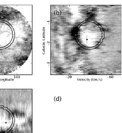
Figure 1.: Shell candidate for Sh2–203. The HII region is marked as a thin line circle (panel (a)), and as a cross (panels (b) and (c)). The thick line ring corresponds to the best fitting model (Table 1).

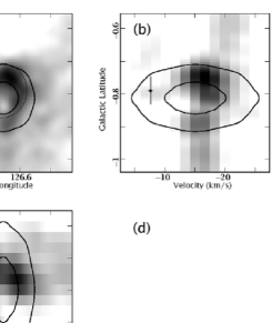
Figure 2.: Same as Fig. 1, but for the case of Sh2–187.

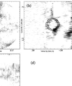
Figure 3.: Shell candidate for HD18352. The star is marked as a cross. The thick line ring corresponds to the best fitting model (Table 1).

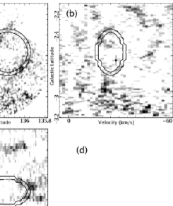
Figure 4.: Same as Fig. 3, but for the case of BD+56 675.

We have tested the shell detection code on four objects: two HII regions (Sh2–187 and Sh2–203) and two B1V stars (HD18352 and BD+56 675). The HII regions cover a wide range of sizes ($10^{\prime}$ for Sh2–187, and $45^{\prime}$ for Sh2–203 — Sharpless 1959). Sh2–187 is known to possess an HI shell (Joncas, Durand, & Roger 1992). Radial velocity values for all four objects are available (Fich et al. 1990; SIMBAD). We have used the CGPS HI data, which have high spatial ($\sim 1^{\prime}$) and velocity (1.32 km s^-1) resolution. The search was limited to shells with an expansion velocity $V_{e}$ in the range 3.3 km s${}^{-1}\leq V_{e}\leq 15$ km s^-1 and an angular radius $R$ in the range $1.^{\prime}2\leq R\leq 16^{\prime}$ (HD18352 and BD+56 675), $2^{\prime}\leq R\leq 26^{\prime}$ (Sh2–187) and $3.^{\prime}6\leq R\leq 47^{\prime}$ (Sh2–203).

In all four cases shell candidates with $\rho/\rho_{99}>1.3$ were found. Figures 1–4 show the detection plots (panels (d)) and three orthogonal slices through the preprocessed data-cubes (panels (a)–(c)). In most cases there is evidence for a multi-shell structure (Figures 1d, 2d, 4d). The data on the highest probability shell detections are summarized in Table 1.

Table 1.: Parameters of the shell candidates

Object	log(N)	$\rho/\rho_{99}$	$l_{0}$,	$b_{0}$,	$V_{0}$,	$R$,	$V_{e}$,
			dgr.	dgr.	km s-1	arcmin	km s-1
Sh2–203	4.40	1.45	143.82	$-1.63$	$-39$	42	14
Sh2–187	3.24	1.48	126.65	$-0.81$	$-15$	5.4	9
HD18352	3.90	1.48	137.93	$+2.20$	$-8$	17	9
BD+56 675	4.29	1.32	136.17	$-2.57$	$-25$	13	9

Acknowledgments.

We would like to thank Francis Boulva for the help with the data processing. This work is supported by a grant from the Natural Sciences and Engineering Research Council of Canada.

References

Arnal, E. M., Cappa, C. E., Rizzo, J. R., & Cichowolski, S. 1999, AJ, 118, 1798

Arnal, E. M., & Mirabel, I. F. 1991, A&A, 250, 171

Benaglia, P., & Cappa, C. E. 1999, A&A, 346, 979

Bisnovatyi-Kogan, G. S., & Silich, S. A. 1995, Reviews of Modern Physics, 67, 661

Bruhweiler, F. C., Gull, T. R., Kafatos, M., & Sofia, S. 1980, ApJ, 238, L27

Cappa, C. E., Goss, W. M., Niemela, V. S., & Ostrov, P. G. 1999, AJ, 118, 948

Cox, D. P. 1972, ApJ, 178, 169

Dubner, G., Giacani, E., Cappa de Nicolau, C., & Reynoso, E. 1992, A&AS, 96, 505

Elmegreen, B. G., & Chiang, W.-H. 1982, ApJ, 253, 666

English, J., et al. 1998, Publ. Astron. Soc. Australia, 15, 56

Fich, M., Dahl, G. P., & Treffers, R. R. 1990, AJ, 99, 622

Gervais, S., & St-Louis, N. 1999, AJ, 118, 2394

Joncas, G., Durand, D., & Roger, R. S. 1992, ApJ, 387, 591

Landau, L. D., & Lifshitz, E. M. 1959, Fluid Mechanics (Oxford: Pergamon)

Mashchenko, S. Y., & Silich, S. A. 1994, Astronomy Reports, 38, 207

Mashchenko, S. Y., Thilker, D. A., & Braun, R. 1999, A&A, 343, 352 (MTB)

Pineault, S., Gaumont-Guay, S., & Madore, B. 1996, AJ, 112, 201

Sharpless, S. 1959, ApJS, 4, 257

Silich, S. A., Mashchenko, S. Y., Tenorio-Tagle, G., & Franco, J. 1996, MNRAS, 280, 711

Staveley-Smith, L., Sault, R. J., Hatzidimitriou, D., Kesteven, M. J., & McConnell, D. 1997, MNRAS, 289, 225

Tenorio-Tagle, G. 1981, A&A, 94, 338

Thilker, D. A., Braun, R., & Walterbos, R. A. M. 1998, A&A, 332, 429

van der Bij, M. D. P., & Arnal, E. M. 1986, Astrophysical Letters, 25, 119

Weaver, R., McCray, R., Castor, J., Shapiro, P., & Moore, R. 1977, ApJ, 218, 377