Abstract. In contrast to the situation with the geodynamo, no breakthrough has been made in the solar dynamo problem for decades. Since the appearance of mean-field electrodynamics in the 1960’s, the only really significant advance was in the field of flux tube theory and flux emergence calculations. These new results, together with helioseismic evidence, have led to the realization that the toroidal magnetic flux giving rise to activity phenomena must be stored and presumably generated below the convection zone proper, in what I will call the DOT (Dynamo-Overshoot-Tachoclyne) layer. The only segment of the problem we can claim to basically understand is the transport of flux from this layer to the surface. On the other hand, as reliable models for the DOT layer do not exist we are clueless concerning the precise mechanisms responsible for toroidal/poloidal flux conversion and for characteristic migration patterns (extended butterfly diagram) and periodicities. Even the most basic result of mean-field theory, the identification of the butterfly diagram with an $\alpha$–$\omega$ dynamo wave, has been questioned. This review therefore will necessarily ask more questions than give answers. Some of these key questions are

• Structure of the DOT layer

• $\alpha$-quenching and distributed dynamo

• High-latitude migration patterns and their interpretation

• The ultimate fate of emerged flux

1. INTRODUCTION

The turn of the millennium invites us to look back and draw balances in all fields of human activity. Yet in solar dynamo theory we also have an added incentive to make such an assessment. In the theory of the geodynamo a significant breakthrough has been achieved in the past few years (? ?, ? ?, ? ?), leading to a surge of renewed activity in the field. One cannot but wonder if a similar breakthrough is within reach in the case of the solar dynamo. Unfortunately, as it will turn out from this review, the prospects are rather bleak, at least on a short term.

As for such a comparative assessment one needs a wider historical outlook this review will not be restricted to the developments that have taken place since the reviews of ? (?) and ? (?). (Such developments were mostly limited to advances in the study of interface dynamos, cf. Sect. 3 below.) A wider historical overview, starting with the dawn of mean-field theory in the 1950s and 60s will thus be given in Section 2 below. Given the finite amount of space available, I will compensate for this wider temporal scope of the review by restricting attention strictly to the problem of the origin of the solar cycle, i.e. of the 22 year periodic variation of solar activity, and associated migration patterns (butterfly diagram). Solar activity variations on both shorter and longer timescales are ignored, as are the solar-type magnetic cycles in other stars, non-axisymmetric phenomena such as active longitudes, and the problem of the long-time phase coherence of the cycle. This restriction is imposed out of necessity only, and in no way does it imply that these effects do not yield important clues even to the origin of the 22 year cycle itself. Clearly, a critical test of any theory of the solar cycle is whether it can be readily extended to predict these other phenomena as well.

After the historical overview, Section 3 will attempt to cut some order in the dazzling multitude of solar dynamo models by introducing a classification scheme. Three main model families can be clearly discerned: overshoot dynamos, interface dynamos and flux transport models, circulation-driven “conveyor belt” models being the most important subgroup of the latter class. Finally, Section 4 calls attention to some key areas where more intensive theoretical or observational efforts could lead to significant advance.

But first of all we should state clearly what are the basic observational facts to be interpreted by a solar cycle model. Once we apply our aforementioned restriction excluding long-term variations, stellar activity etc., the remaining list is quite short.

• The 11/22 year cycle period. Beside reproducing the value of the period, the crude agreement of this value with the timescale of pole-equator diffusion in the convective zone also asks for an explanation. While such an order-of-magnitude equality can certainly be coincidental (cf. the coincidence of the solar rotation period with the convective turnover time in the deep convective zone), a natural explanation for it would clearly make any cycle model more attractive.

  

  
  

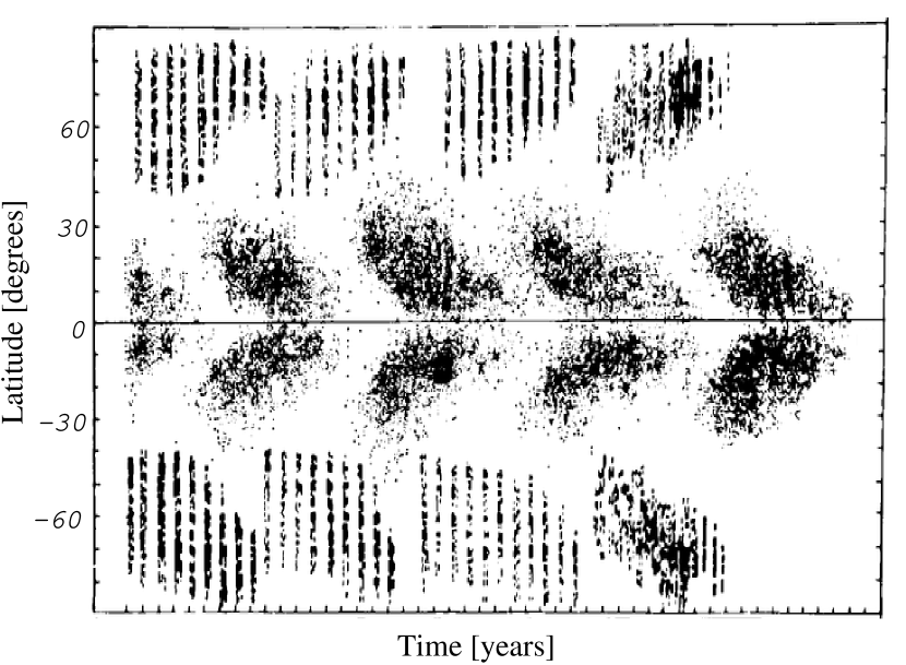
  Figure 1: Extended butterfly diagram of solar activity: time-latitude distribution of sunspot groups (low-latitude branches) and polar faculae (high-latitude branches). After Makarov & Sivaraman (1989)

• The characteristic migration pattern (extended butterfly diagram). Our knowledge of latitudinal migration patterns of magnetic flux is summarized in the extended butterfly diagram of Figure 1. The tracers shown here track partly toroidal and partly poloidal fields. While azimuthal field lines by definition cannot cross the surface, the observed properties of large-scale solar active regions strongly suggest that they are tracers of a subsurface toroidal field, locally bulging out into the atmosphere. In this sense, photospheric magnetometry can give us information about the migration patterns of the toroidal field component as well. At low ($\mathrel{\mathchoice{\vbox{\offinterlineskip\halign{\hfil$\displaystyle#$\hfil\cr<\cr\sim\cr}}}{\vbox{\offinterlineskip\halign{\hfil$\textstyle#$\hfil\cr<\cr\sim\cr}}}{\vbox{\offinterlineskip\halign{\hfil$\scriptstyle#$\hfil\cr<\cr\sim\cr}}}{\vbox{\offinterlineskip\halign{\hfil$\scriptscriptstyle#$\hfil\cr<\cr\sim\cr}}}}35^{\circ}$) latitudes both the poloidal and the toroidal field components migrate equatorward. At high latitudes, poloidal fields show a marked poleward migration, as indicated also by the migration pattern of a number of tracers such as quiescent prominences or the coronal green line. The migration pattern of high-latitude toroidal fields is less clear —a point we will return to in Section 4.2 below.

• The confinement of strong activity (large active regions) to low heliographic latitudes $|\Phi|\mathrel{\mathchoice{\vbox{\offinterlineskip\halign{\hfil$\displaystyle#$\hfil\cr<\cr\sim\cr}}}{\vbox{\offinterlineskip\halign{\hfil$\textstyle#$\hfil\cr<\cr\sim\cr}}}{\vbox{\offinterlineskip\halign{\hfil$\scriptstyle#$\hfil\cr<\cr\sim\cr}}}{\vbox{\offinterlineskip\halign{\hfil$\scriptscriptstyle#$\hfil\cr<\cr\sim\cr}}}}35^{\circ}$.

• The phase dilemma(s). In its original sense (? ?) the phase dilemma consists of the fact that at low latitudes the radial field (derived by azimuthal averaging of the magnetograms) is in an approximately $\pi$ phase lag compared to the toroidal field at the same latitude. Another phase lag to be explained is the $\pi/2$ lag between the two branches of the butterfly diagram, i.e. that the polar field reversal occurs slightly after the sunspot maximum. Finally, the phase of torsional oscillations (cycle-related periodic oscillations of the rotational velocity in migrating belts) relative to the toroidal field is a third quantity constraining theories of the cycle.

2. HISTORY

2.1. Convection zone dynamos

It all started with Parker’s (?) classic paper that set down the foundations for solar $\alpha\Omega$ dynamo theory. In its trace, mean field electrodynamics was developed during the 1960’s (? ?, ? ?). To give a reminder of the basics, described in so many other reviews (e.g. ? ?, ? ?) the induction equation in a turbulent conductive medium reads

$$\partial_{t}\mbox{\bf B}=\nabla\times(\mbox{\bf U}\times\mbox{\bf B}+\vec{\cal E})-\nabla\times\eta\nabla\times\mbox{\bf B}.$$ (1)

where B is the mean magnetic field, U is the large-scale flow velocity, $\partial_{t}$ denotes time derivative, $\eta$ is the magnetic diffusivity, and $\vec{\cal E}$ is the turbulent electromotive force arising as a result of the interaction between the turbulent velocity field v and the turbulent magnetic field. This latter is in turn the result of the action of v on the mean field B, so $\vec{\cal E}$ is a functional of v and B. Assuming scale separation $l\ll H_{B}$ where $H_{B}$ is the length scale of the mean field and $l$ is the scale of turbulence, $\vec{\cal E}$ can be expanded in the derivatives of B. For homogeneous and isotropic turbulence this yields

$$\vec{\cal E}=\alpha\mbox{\bf B}-\beta\,\nabla\times\mbox{\bf B}$$ (2)

where $\alpha$ and $\beta$ are now functionals of v only. Substituting (2) into (1) we see that the role of $\beta$ is formally identical to that of $\eta$. For this reason $\beta$ is called turbulent magnetic diffusivity, and elementary considerations or even dimensional analysis yield $\beta\sim lv$. As for turbulence the Reynolds number $\beta/\eta\gg 1$, in practice $\eta$ can be omitted in equation (1). In contrast, the pseudoscalar $\alpha$ gives rise to a qualitatively new effect, the $\alpha$-effect.

In the axisymmetric case considered here, using spherical coordinates $\theta$, $\phi$, $r$, B can be split as

$$\mbox{\bf B}=B\mbox{\bf e}_{\phi}+\nabla\times(A\mbox{\bf e}_{\phi})$$

where $\mbox{\bf e}_{\phi}$ is the azimuthal unit vector, $B$ is the toroidal field component, and $A$ is the (toroidal) vector potential of the poloidal field. We further assume that U is a pure rotation

$$\mbox{\bf U}=r\sin\theta\,\Omega\,\mbox{\bf e}_{\phi}$$

and introduce the shear vector

$$\hat{\vec{\Omega}}=r\sin\theta\,\nabla\Omega$$

In the limit $r\sin\theta/H_{B}\rightarrow\infty$ the form of the vector operators simplifies to their form for the local Cartesian frame $\mbox{\bf e}_{x^{\prime}}=\mbox{\bf e}_{\theta}$, $\mbox{\bf e}_{y^{\prime}}=\mbox{\bf e}_{\phi}$, $\mbox{\bf e}_{z^{\prime}}=\mbox{\bf e}_{r}$. Now we introduce a new frame $xyz$ by rotating $x^{\prime}y^{\prime}z^{\prime}$ around $\mbox{\bf e}_{\phi}$ with an angle $-\pi/2\leq\Delta\theta<\pi/2$ so that $\hat{\Omega}_{x}=0$. With these assumptions and notations the poloidal and toroidal parts of equation (1) read

$$\partial_{t}A=\alpha B+\beta\,\nabla^{2}A$$ (3)

$$\partial_{t}B={\hat{\Omega}}_{z}\,\partial_{x}A-\alpha\nabla^{2}A+\beta\,\nabla^{2}B,$$ (4)

known as the classic dynamo equations.

It is clear from (3–4) that the role of the pseudoscalar $\alpha$ is to turn the poloidal and toroidal field components into each other which implies some kind of helical motion. The classic candidate for this, suggested by ? (?) is the passive advection of fields by helical convective motions. Later, alternative mechanisms for an $\alpha$-effect were also proposed, based on a dynamic interaction of field and motions (see Section 4.3 below). A general property of these mechanisms is that $\alpha$ turns out to be positive in the bulk of the solar convective zone in the northern hemisphere, while it tends to be negative in the stably stratified layer below. (Being a pseudoscalar, $\alpha$ changes sign between hemispheres.)

The shear $\hat{\Omega}$, associated with differential rotation, in turn, winds up the poloidal field into a toroidal component. Without the $\alpha$ and $\Omega$ terms we would be left with a diffusively decaying field, so at least one of these terms is necessary for dynamo action in both equations. Depending on which, if any, of the dynamo terms in (4) is discarded, we distinguish $\alpha^{2}$, $\alpha\Omega$ and $\alpha^{2}\Omega$ dynamos. $\alpha^{2}$ dynamos can be shown to give rise to non-oscillatory behaviour and toroidal and poloidal field amplitudes of the same order of magnitude which does not agree with the properties of the solar dynamo. Thus, in what follows we will concentrate on $\alpha\Omega$ dynamos, neglecting the second term on the r.h.s. of (4). (Note, however, that under more general conditions than those considered here, oscillatory $\alpha^{2}$ dynamos can also be constructed, as pointed out recently by ? ?.)

Assuming that beside $\alpha$ and $\beta$, ${\hat{\Omega}}_{z}$ can also be regarded constant, the system (3–4) is homogenous and linear, admitting wavelike solutions of the form

$$B=B_{0}\exp\,[i(\omega t-\mbox{\bf k}\mbox{\bf x})]$$ (5)

$$A=A_{0}\exp\,[i(\omega t-\mbox{\bf k}\mbox{\bf x}+\delta)]$$ (6)

where $\omega=\omega_{R}+i\omega_{I}$ is a complex frequency while all other variables are real. $\omega_{R}$, $A_{0}$ and $B_{0}$ can be taken to be non-negative without loss of generality. Introducing the (signed) Reynolds numbers

$$R_{\alpha}=\alpha/\beta k\qquad R_{\Omega}={\hat{\Omega}}_{z}/\beta k^{2}$$ (7)

as well as the dynamo number and the nondimensional frequency

$$D=R_{\alpha}R_{\Omega}\qquad\tilde{\omega}=\omega/\beta k^{2}$$ (8)

and substituting the Ansatz (5–6) into (3–4) we find

$$(1+i\tilde{\omega})A_{0}=k^{-1}R_{\alpha}B_{0}\,e^{-i\delta}$$ (9)

$$(1+i\tilde{\omega})B_{0}=-ik_{x}R_{\Omega}A_{0}\,e^{i\delta}$$ (10)

The product of these latter equations is

$$(1+i\tilde{\omega})^{2}=-iDk_{x}/k$$ (11)

As only $k_{x}$ appears in (10), no unstable modes (self-excited field or “dynamo waves”) exist with $k_{x}=0$. Remembering the way we oriented our $x$-axis this implies that dynamo waves propagate along isorotational surfaces. But in which direction? The imaginary part of (11) reads

$$2\tilde{\omega}_{R}(1-\tilde{\omega}_{I})=-Dk_{x}/k$$ (12)

As for unstable modes (self-excited field or “dynamo waves”) $\omega_{I}\leq 0$, (12) yields the important result

$$k_{x}D<0,$$ (13)

known as the Parker–Yoshimura sign rule. Thus, e.g. in the northern hemisphere equatorward propagation ($k_{x}>0$) implies $D<0$. With a positive $\alpha$, as is the case in the bulk of the convective zone, this implies $\partial_{r}\Omega<0$, an outward decreasing rotational rate. This was indeed the general expectation for the solar internal rotational law in the 1960’s and 1970’s.

The solution of (11) is

$$\tilde{\omega}=i\pm(1-i)(-Dk_{x}/2k)^{1/2}$$ (14)

For unstable modes obviously the plus sign applies. So the growth rate is

$$-\tilde{\omega}_{I}=(-Dk_{x}/2k)^{1/2}-1$$ (15)

Unstable modes thus exist when $|D|\geq 2$ in nondimensional units. As according to equation (8) $|D|$ decreases with $k$, it is the lowest $k$ modes, with a scale comparable to the solar radius $R_{\odot}$ that have the highest growth rate and will dominate the solution. (Note that this implies that our formalism, derived for the limit $kr\sin\theta\rightarrow\infty$, is strictly speaking invalid for these modes —nevertheless it may still be used for general guidance.)

Note that when $\tilde{\omega}_{I}=0$, $\tilde{\omega}_{R}=1$ follows from (14): the period of the critical mode is thus just the diffusive timescale corresponding to $R_{\odot}$. Estimating $\alpha$ and $\hat{\Omega}_{z}$ on the basis of helical convection and the observed differential rotation, $D$ proves to be order of unity for a convection zone dynamo, showing that the dynamo is indeed approximately critical, and thus naturally explaining the agreement of the cycle period with the diffusive timescale.

Finally, let us note that it is straightforward to work out from the above formulae that for an equatorward propagating wave, the phase of the radial field component relative to the toroidal field is $-3\pi/4$ if $\alpha>0$ in the northern hemisphere and $\pi/4$ otherwise (? ?).

Taken altogether, the above considerations showed that for the expected positive $\alpha$-effect in the solar convective zone, assuming an inwards increasing rotational rate, one can correctly reproduce the cycle period, the equatorward branches of the butterfly diagram as a dynamo wave, and the low-latitude phase relationship. (The high-latitude poleward branch could obviously be reproduced by assuming $\partial_{r}\Omega>0$ there, though this line was not pursued, relying on the Babcock-Leighton approach instead.) All this gave the impression that, missing details apart, the basic mechanism of the solar dynamo is well understood.

2.2. Crisis

The first warning signs that something is amiss began to appear towards 1970, with the realization that most of the magnetic flux in the solar photosphere, and presumably below, is present in a strongly intermittent form, concentrated into strong flux tubes (? ?, ? ?, ? ?, ? ?). Flux tube theory developed in the 1970’s and it became clear that for thicker flux bundles, owing to their lower surface/volume ratio, volume forces such as buoyancy, curvature and Coriolis forces dominate over the drag of the surrounding plasma flows acting on the surface. These tubes can then move largely independently of the surrounding flows, invalidating simple one-fluid descriptions like mean field theory. Thus, solar magnetic fields can be divided into two components: passive fields, consisting of thin flux fibrils, that move passively with the flow owing to the drag and are the subject of mean field theory; and active fields, consisting of thick flux bundles moving under the action of volume forces. And the characteristics of large active regions strongly suggested that they are essentially (fragmented) loops formed on toroidal flux bundles of $10^{22}\,$Mx which clearly fall in the active category, outside the jurisdiction of mean field models.

What is more, ? (?) called attention to the fact that such flux bundles cannot be stored in the convective zone for a time scale comparable to the cycle period, being subject to buoyant instabilities that can rapidly remove the whole tube from the zone. The only place to store these tubes is near the bottom of the convective zone, especially in the stably stratified but still turbulent lower overshoot layer below it. Toroidal flux tubes lying here may still develop finite-wavelength buoyant instabilities that may give rise to loops erupting through the convective zone into the atmosphere, producing active regions. This scenario has gained firm foundations with the first nonlinear calculation of the emergence of such loops through the convective zone (? ?), and such flux emergence models have by now evolved into an independent chapter of the global dynamo problem. In the present review we will not deal with this topic in detail (see the review by ? ?), even though flux emergence models are the only real “success story” of dynamo theory since the 1960’s. While many details are still unclear, by now these models can reproduce sunspot proper motions and active region flux distributions to a quite convincing detail. A very robust main conclusion from the models, of great importance for the global dynamo, is that in order to reproduce the observed characteristics of active regions the toroidal flux tubes must have a field stregth of about $10^{5}\,$G —an order of magnitude higher than the turbulent equipartition field in the deep convective zone. Explaining the origin of such strong fields is a major challenge for dynamo theory.

Guided by these realizations, in the 1980’s the first attempts were made to construct dynamos operating in the lower overshoot layer. The unknown profiles of $\alpha$ and the differential rotation, however, greatly impeded progress, allowing a far too wide parameter space to play with. Therefore, attempts were made to numerically simulate the whole convective zone, with a consistent picture of differential rotation, helical convection, and dynamo (? ?). Nevertheless, the results (poleward propagating dynamo waves) were at odds with the observations, and when finally even the predicted differential rotation profile (constant on cylinders) was proven wrong by helioseismic measurements (constant on cones), the simulational approach was abandoned (cf. the remarks in Section 5).

On the other hand, the helioseismic determination of internal differential rotation gave new impetus to mean field dynamo theory. Those inversions clearly showed that most of the shear (the $\Omega$-effect) is concentrated in a thin layer near the bottom of the convective zone, known as the tachocline. This was seen as further evidence that a thin layer situated about $200\,000\,$km below the solar surface is of key importance for the working of the solar dynamo. Depending on the physical viewpoint we study it from, this layer is alternatively called dynamo layer, overshoot layer or tachocline. In the present review for simplicity I will refer to it as the DOT (Dynamo — Overshoot — Tachocline) layer.

Table 1: A classification scheme for solar dynamo models

3. MAIN FAMILIES OF MODELS

Solar mean field dynamo theory in the past decades gave rise to a bewildering variety of models. Nevertheless, all recent models (i.e. those using the helioseismic rotation law) can be classified into just four main types according to a plausible classification scheme (Table 1 and Figure 2). One classification parameter here divides the models according to whether they still interpret the butterfly diagram as a dynamo wave just like the orthodox convection zone dynamos did, or if they substitute that with some flux transport mechanism (meridional circulation or pumping). The other parameter in turn divides the models according to whether the $\alpha$- and $\Omega$-effects are cospatial or “distributed”, i.e. they take place in different (adjacent or very distant) parts of the model volume. The resulting four model types are as follows.

Figure 2: Schematic illustration of the main features of main solar dynamo families. The sites of $\alpha$ and $\Omega$ effects and toroidal/poloidal field transport mechanisms and directions are shown in a meridional quadrate. The internal layers marked schematically are, from the inside outwards, the radiative, DOT and convective layers. OL: Overshoot layer dynamos; IF: Interface dynamos; CP: Cospatial pumping models; BL: Babcock-Leighton type models;

3.1. Cospatial wave models: OL dynamos

Widely known as “overshoot layer” or OL dynamos, these are perhaps the most conservative models that simply replant the concepts of the convective zone dynamos of the 1960’s and 70’ into the DOT layer. As the helioseismic inversions show $\partial_{r}\Omega>0$ at low latitudes, these models need to assume $\alpha<0$ to get the right migration directions. This assumption is rather plausible in the DOT layer for several different physical mechanisms for $\alpha$. The state-of-the-art in this approach is represented by the model of ? (?).

Successes:

• The butterfly diagram comes out right. The Parker-Yoshimura rule leads to polar and equatorial branches separated at the corotational latitude, as observed.

Difficulties:

• The low-latitude phase dilemma: as now $\alpha<0$, the radial field is found to be nearly in phase with the toroidal field, instead of being in antiphase as observed.

• The cycle period tends to be too short for thin layer models. This is basically because the same amount of differential rotation is now concentrated in a much thinner layer, leading to much stronger shear and much higher dynamo numbers. This may be compensated by reducing $\alpha$, e.g. by arguing that, as nonlinear effects act via a quenching of the $\alpha$ and $\Omega$ mechanisms, it is natural to expect that after saturation the dynamo will be effectively critical. Yet the degree to which the nonlinearity can increase the cycle period depends a lot on the assumptions made, and in general it does not seem sufficient (? ?). At any rate, certain “tricks”, such as using an $\alpha^{2}\Omega$ dynamo (? ?) or introducing an intermittence factor (? ?), can save the models, but then the crude coincidence of the period with the lateral diffusive timescale is coincidental.

• For an equatorial confinement of strong fields the $\alpha$-effect needs to be arbitrarily confined to low latitudes. Nevertheless, such $\alpha$-distributions are indeed found in some calculations (cf. ? ?).

3.2. Distributed wave models: IF dynamos

? (?) suggested a dynamo where the diffusivity discontinuously varies by many orders of magnitude across a surface. The $\alpha$-effect operates on the high-diffusivity side of the interface, while the $\Omega$-effect (shear) is limited to the low-diffusivity side. He showed that under these conditions a dynamo wave can be excited, obeying the Parker-Yoshimura sign rule. The attractive feature of this model is that the toroidal field generated on the low diffusivity side can be made arbitrarily strong by reducing the value of magnetic diffusivity there. Thus, the origin of $10^{5}\,$G fields could be explained.

Parker’s analytic, plane parallel model has been extended to more realistic situations and incorporated in full solar dynamo models in a number of papers (? ?, ? ?). Unfortunately, the results are somewhat contradictory owing to numerical problems related to modelling the discontinuity. In this context we may perhaps note that the main physical difference of these IF models compared to the OL models is the spatial separation of $\alpha$ and $\Omega$. The introduction of a discontinuity between them is an added feature that can simplify the analytic treatment but at the same time complicate the numerical calculations. A model where the diffusivity is continuously distributed, albeit with a sharp gradient, with $\alpha$ and $\Omega$ concentrated on the two sides of this gradient, may well be worth considering. Beside being more realistic, such a model might also avoid the numerical problems mentioned.

Successes:

• Strong toroidal fields can be readily explained.

Difficulties:

• At the present stage, numerical difficulties prevail. An evaluation of the physical performance of the models will only be possible after these are resolved.

3.3. Cospatial transport models: CP dynamos

In an inhomogeneous medium, the proper expression of $\vec{\cal E}$ is more general than equation (2), the scalars $\alpha$ and $\beta$ being substituted by tensorial expressions. A tensorial $\hat{\alpha}$-term in (2) can then alternatively be written as

$$\hat{\alpha}\mbox{\bf B}=\alpha\mbox{\bf B}+\hat{\alpha}_{S}\mbox{\bf B}-\vec{\gamma}\times\mbox{\bf B}$$

where $\alpha=\mbox{Tr\,}\hat{\alpha}$, the last term is the vectorial product equivalent of the action of the antisymmetric part of $\hat{\alpha}$ on B, and $\hat{\alpha}_{S}$ is the symmetric and traceless part of $\hat{\alpha}$. Substituting (2) into (1) we see that the role of $-\vec{\gamma}$ is analoguous to that of U, i.e. it formally describes an advection of the magnetic field. This effect is called the (normal) pumping of the field along the inhomogeneity. The $\hat{\alpha}_{S}$-term can be shown to give rise to a similar effect with the difference that the sign of the transport depends on the orientation of the field component perpendicular to the pumping direction (anomalous pumping; see ? ? for a detailed discussion).

It must be stressed that the descriptions using a tensorial alpha and those using pumping effects are formally equivalent. The advantage of the pumping formalism is that it helps one to get a physical “feeling” of the processes at work.

Depending on the particular inhomogeneity associated with the pumping, one can speak of density pumping, turbulent pumping etc. It was suggested by ? (?) that, instead of appealing to a dynamo wave, the field migration patterns can also be interpreted by density pumping, directed towards the rotational axis for poloidal fields and away from it for toroidal fields. This pumping is supposed to operate throughout the convective zone, instead of being confined to the DOT layer. A more detailed model along these lines has recently been constructed by ? (?). While the model reproduces well the phase relation for the torsional oscillations, it does not even address questions such as the origin of the deep-seated toroidal field. Thus, while the basic concept is interesting, at the present stage this “cospatial pumping” approach cannot be regarded as a serious aspirant for the explanation of the global dynamo.

3.4. Distributed transport models: BL dynamos

These are generally known as “Babcock–Leighton-type” models (hence the BL code). While they indeed grew out of the semiempirical approach of ? (?) and ? (?) to the solar cycle, they did get a lot more radical in the 1990’s. Indeed, in the era of convective zone dynamos, in the 1960’s and 70’s, the Babcock-Leighton approach was not seen as necessarily conflicting with the dynamo wave theory of the cycle. With a dynamo operating throughout the convective zone, the $\alpha$-effect caused by the inclination of active region axes relative to E–W (which is the cornerstone of this approach) could be considered as helical convection caught in the act; and in his mathematical formulation of the model ? (?) explicitly assumed that the toroidal field migration is the result of a dynamo wave. It was only the poleward migration of the poloidal field that was interpreted in terms of a lateral transport.

In subsequent versions of the model, meridional circulation plays the main role in transporting the poloidal fields to the poles near the surface. And from here it was just one step to close the circle and assume that the deep return flow of meridional circulation is responsible for the equatorward drift of the toroidal field. This step, made by ? (?) was radical indeed: it represented the first break with the canonical interpretation of the butterfly diagram as a dynamo wave, generally accepted for three decades.

The model essentially works like a conveyor belt: the poleward meridional circulation near the surface transports the poloidal fields towards the poles at high latitudes, giving rise to the poleward branch of the butterfly diagram. At the poles, the fields are advected down to the bottom of the convective zone where the shear converts them into toroidal fields that get amplified while advected towards the equator. Once these are strong enough, they are supposed to form buoyantly emerging loops at low latitudes that give rise to active regions, the Coriolis force lending an inclination to the loop planes, i.e. introducing an $\alpha$-effect, and thus regenerating the poloidal field.

More recent versions of the model (? ?, ? ?) have developed it into an internally consistent modelling approach with the ambition of yielding a complete description of the solar cycle. As such, this family of models is at present the most serious competitor of the OL class.

Successes:

• The low-latitude confinement of strong activity comes out rather naturally. (The toroidal field is amplified by shear as it is advected equatorward.)

• A tolerable reproduction of the extended butterfly diagram (although the latitude where the two branches part tends to be too high). Note, however, that the original (one-dimensional) Babcock–Leighton models gave a much closer fit to the observed migration patterns, which was their main asset. In the extension to two dimensions, BL dynamos had to sacrifice this achievement.

Difficulties:

• The agreement of the corotational latitude with the latitude where the butterfly branches diverge must be considered coincidental (if reproduced at all).

• The $\alpha$-effect is confined to the surface. This is probably unrealistic even for flux tube alpha, cf. the discussion in Section 4.3 below.

• The model, as all models relying on a flux tube alpha, is not self-exciting, as this $\alpha$-effect works for strong fields only. It needs another dynamo mechanism to “kick it in”.

• A serious problem is that the approach only works with an unrealistically low value for the turbulent diffusivity in the convective zone, $\beta\sim 10\,$km${}^{2}/$s. (This is needed to keep the two parts of the “conveyor belt” separated. In fact the main difference between the BL and IF models is that the separated seats of $\alpha$ and $\Omega$ communicate by diffusion in the IF models.) There is no justification for such a low value. On physical grounds, $\beta\sim 0.5lv\simeq 500\,$km${}^{2}/$s is expected —indeed, even the one-dimensional Babcock–Leighton models predicted $600\,$km${}^{2}/$s. According to the controversial proposal of ? (?), on the other hand, the diffusivity should have been quenched by many orders of magnitude to values far lower than those used in the BL models. (Note that by now this question has been settled: diffusivity suffers no strong quenching in realistic, intermittent fields in three dimensions, ? ?, ? ?.)

  

  Figure 3: Steamy window: with realistic turbulent transport parameters, an arbitrary time-dependent poloidal field pattern imposed at the bottom of the convective zone is reflected, somewhat blurred, at the surface. After Petrovay & Szakály (1999)

  One may wonder if the effect of the strong diffusive link can be reduced by some kind of selective field pumping that would keep the two field components apart. ? (?) investigated this possibility in a model of poloidal field transport, incorporating all known transport effects (circulation, diffusion, turbulent pumping, density pumping). It turns out that diffusion is dominant, forging such a strong link between the DOT region and the surface that any migration pattern imposed at the bottom will be reflected at the top (Fig. 3). This seems to represent a serious difficulty for BL models.

4. KEY ISSUES

4.1. Structure of the DOT region

It is obvious from the above model descriptions that a thorough understanding of the structure and dynamics of the DOT layer is crucial for advance in solar dynamo theory. Unfortunately, at present we do not have a reliable model for this layer. As a complicated interplay of convection, rotation and magnetic fields is expected there, as a first step one would expect to develop models for just one aspect of the problem: a model for overshoot with no rotation and magnetic fields; a non-magnetic model for the tachocline with no overshoot; etc. Nevertheless, we lack even such simplistic models, and surprisingly little effort is made to construct them.

In the case of overshoot, the way to construct such a model is in principle well known: it consists in solving a conveniently truncated hierarchy of the Reynolds stress equations. ? (?) present preliminary results from a numerical study of this problem.

Helioseismic inversions show that the thickness of the tachocline is about $0.1\,R_{\odot}$. This is puzzling, as even in the absence of turbulent diffusion, the Eddington–Sweet circulation should have mixed these layers enough in $4.6\cdot 10^{9}$ years to extend the tachocline to much greater depths (? ?). It is most often assumed that the solution to this “thin tachocline problem” resides in anisotropic turbulence: an extremely strong horizontal anisotropy would indeed effectively smooth out horizontal gradients without contributing much to the vertical transport. But in view of strong nonlinear mode coupling in turbulence, such an extreme anisotropy seems dubious. ? (?) explore the alternative possibility that the necessary horizontal momentum transfer is due to an inverse $\Lambda$-effect: however, the necessary amplitude of $\Lambda$ proves even more unrealistically large. Magnetic decoupling of the envelope from the radiative interior is a third explanation put forward by ? (?).

4.2. High-latitude field patterns

In order to be able to decide between various dynamo models, one needs an issue on which they yield conflicting predictions that are relatively easy to test. One such case is the migration of the toroidal field at high latitudes. In dynamo wave (OL and IF) models at high latitudes all field components migrate polewards, following the Parker–Yoshimura rule. In contrast, the toroidal field in BL models typically shows an equatorward migration, advected by the return flow of meridional circulation near the bottom of the convective zone. Thus, if a clear signature of migrating high-latitude toroidal fields were found, this could solve the problem in either way, depending on the direction of migration. It is often claimed (e.g. ? ?) that high latitude ephemeral active regions show an equatorward migration. But a closer examination of such claims shows that they are based only on the fact that high latitude ephemeral regions as a whole tend to lie in the backwards extension of the low-latitude butterfly “wings” (just as polar faculae do), and not on a detailed study of migration patterns among high-latitude regions only. On the other hand, ? (?) claim that at least 50 % of polar faculae (well known for their poleward drift) correspond to dipoles with a preferential east–west orientation, thus forming part of the toroidal field. It has even been claimed that the highest-latitude part of the sunspot butterfly diagram also shows a poleward drift (? ?). A clarification of this issue would clearly be important.

A related problem is the origin of ephemeral active regions in general. If they are used as magnetic tracers we would obviously like to know what kind of field do they trace?

4.3. Origin and profile of $\alpha$

It is sometimes claimed that the origin of the $\alpha$-effect assumed is a basic difference between various dynamo models, so that excluding a certain $\alpha$-mechanism amounts to excluding a dynamo variety. In reality, our knowledge of all possible types of $\alpha$-effects is so scarce that wildly differing $\alpha$-profiles can be derived for the same mechanism, depending on particular modelling assumptions. And vice versa: a given profile, used as input in a dynamo model, may be the consequence of various $\alpha$-mechanisms.

More in-depth study of the possible $\alpha$-mechanisms that can reduce this uncertainty could nevertheless really be used to constrain dynamo models in the future. For now, I will argue that, independently of its mechanism, $\alpha$ should be expected to be concentrated towards the bottom of the convective zone, or at least to pervade it uniformly (and not to be concentrated to the surface, as assumed in BL models). Let us see this for the four $\alpha$-mechanisms that have been proposed.

• Cyclonic convection. In this classic variety of the $\alpha$-effect, proposed by ? (?), $\alpha$ results from the effect of rotation on convection, so it increases with the Coriolis number, peaking near the bottom of the solar convective zone. Its sign is positive in the unstable layer and negative in the overshoot layer below.

• Magnetostrophic waves. This mechanism was proposed by ? (?) specifically to suggest an alternative $\alpha$-mechanism for the overshoot layer that will not be suppressed by the strong toroidal fields there. It consists in growing helical waves and its sign is negative, as required by the dynamo wave models. More detailed calculations of its profile were performed by ? (?), though the results may rely too heavily on the background stratification of the (incorrect) overshoot model used.

• Flux loop alpha. The magnetix flux loops emerging through the convective zone and creating the active regions are essentially large-amplitude nonlinear versions of the above mentioned unstable magnetostrophic waves, giving rise to a similar (but positive) $\alpha$-effect. It is clear that after their decay, owing to their tilt, active regions contribute to the passive poloidal field. But is this contribution limited to the surface, or do the “feet” of the loop similarly decay, down to the bottom of the convective zone? This problem relates to the next subsection, but one expects that the eroding action of external turbulence (? ?) will lead to the decay of the whole loop, thereby extending the $\alpha$-effect down to its footpoints. In fact, our turbulent erosion calculations show that 90% of the magnetic flux in an emerging flux loop is lost before it reaches the surface! This lost flux, already submitted to the action of Coriolis force, should contribute to the poloidal field and to the $\alpha$-effect far more than the actual active regions. And then we did not even mention the possibility of “failed active regions”: flux loops that, their field strengths being too weak, never make it to the surface (? ?, ? ?). All this strongly speaks for a flux loop $\alpha$ concentrated to the bottom of the convective zone.

• Unstable Rossby waves. Recently, ? (?) considered a shallow-water model of the tachocline, analysing the behaviour of small perturbations of its geostrophic equilibrium state. They find that such large-scale perturbations are unstable if the subadiabaticity is low enough and they are characterized by a correlation between the vertical components of velocity and vorticity, i.e. by a non-vanishing mean helicity. In other words, these perturbations essentially behave like global-scale unstable Rossby waves, and owing to their mean helicity they can be expected to yield an $\alpha$-effect.

4.4. The ultimate fate of emerged flux

This problem is interesting in its own right, as well as because of its importance for the $\alpha$-effect problem. Once the active region has decayed, what happens to the “trunks” of the magnetic trees? Will they just stay there, “bleeding”? Will they reconnect and be drawn back below the convective zone? Or will they also decay? As indicated above, the turbulent erosion models (? ?) seem to support the latter possibility. At any rate, thorough observational studies of the active region decay (cf. the review by ? ?) may shed more light on this problem.

5. CONCLUSION: …AND THE SIMULATIONS?

As we have seen, there is still no really convincing answer to the question “What makes the Sun tick?”. Several conflicting approaches exist, none of which can fully explain the observed features of the solar cycle and all of which rely on some more or less arbitrary assumptions. In contrast to the optimistic outlook of about three decades ago, nothing seems safe now, not even the dynamo wave origin of the sunspot butterfly diagram. And the prospects do not seem to promise a spectacular change in this situation in the near future.

A number of previous reviews (e.g. ? ?) expressed the view that the ultimate solution to the solar dynamo problem should be expected from numerical hydrodynamical simulations. So the reader may ask: why was the simulational approach hardly even mentioned in this review? Why is it that only mean field models were treated? The answer does not lie in the (undeniable) bias of the author but in the fact that in the past decade there simply have not been any numerical simulations constructed with the ambition of producing a global model for the solar cycle. As we indicated above, such attempts were made back in the 1980’s; but, after their failure in reproducing the butterfly diagram and the internal rotation profile became clear, this line of research was completely abandoned. Those very few hydrodynamical simulations in the 1990’s that had some direct bearing on the solar dynamo problem aimed at the modelling of smaller volumes inside the convective zone with the main purpose of studying the fine structure and transport of the magnetic field (? ?, ? ?, ? ?).

The belief in the “miraculous healing power” of simulations may indeed have been too zealous before. After all, even in an ideal future where an infinite computing potential would make it feasible to make a 3D direct numerical simulation of the whole Sun for $4.6\cdot 10^{9}$ years, the result would have no more direct benefit for us (apart from demonstrating that the laws of classical magnetohydrodynamics are indeed sufficient to describe solar phenomena) than offering a chance to determine any physical quantity at any internal point of our star with arbitrary precision. This feat, though far beyond the possibilities of contemporary observational solar physics, is still basically experimental work that, though important, in no way can substitute “real” theory.

And yet, the other extreme, represented by the present complete abandonment of the simulational approach, is just as lamentable as its opposite. This is especially so as the great advance in the geodynamo problem I referred to in the Introduction can mainly be attributed to the success of numerical simulations. The following pseudo-historical quote by Borges fits nicely the present situation in this respect.

Jorge Luis Borges: On Rigour in Science
…In that Empire, the Art of Cartography achieved such Perfection that the map of a single Province occupied a whole City, and the map of the Empire, a whole Province. With time, these Gigantic Maps proved unsatisfactory and the Colleges of Cartographers set up a Map of the Empire that had the size of the Empire and coincided with it point by point. Less addicted to the Study of Cartography, the Following Generations considered this extensive Map useless and, not without Disrespect, they abandoned it to the Mercy of the Sun and of the Seasons. In the Western deserts broken Ruins of the Map still persist, inhabited by Animals and Beggars; in all the Country no other Relicts of the Geographic Disciplines remain.
Suárez Miranda: Viajes de varones prudentes,
libro cuarto, cap.XLV, Lérida, 1658

References

- 1961 Babcock, H. W. 1961, ApJ 133, 572
- 1959 Becker, U. 1959, Z. für Astrophys. 48, 88
- 1985 Belvedere, G. 1985, Sol. Phys. 100, 363
- 1992 Callebaut, D. K., Makarov, V. I. 1992, Sol. Phys. 141, 381
- 1997 Charbonneau, P., MacGregor, K. B. 1997, ApJ 486, 502
- 1995 Choudhuri, A. R., Schüssler, M., Dikpati, M. 1995, A&A 303, L29
- 1981 Cowling, T. G. 1981, ARA&A 19, 115
- 1999 Dikpati, M., Charbonneau, P. 1999, ApJ 518, 508
- 2000 Dikpati, M., Gilman, P. A. 2000, preprint
- 2000 Dorch, B., Nordlund, Å. 2000, astro-ph/0006358
- 1994 Ferriz Mas, A., Schüssler, M. 1994, A&A 433, 852
- 2000 Forgács-Dajka, E., Petrovay, K. 2000, in P. L. Pallé A. Wilson (Eds.), Helio- and Asteroseismology at the Dawn of the Millennium, ESA Publ., in press
- 1989 Gilman, P. A., Morrow, C. A., De Luca, E. E. 1989, ApJ 338, 528
- 1985 Glatzmaier, G. A. 1985, ApJ 291, 300
- 1995 Glatzmaier, G. A., Roberts, P. H. 1995, Nature 377, 203
- 1994 Gruzinov, A. V., Diamond, P. H. 1994, Phys. Rev. Lett. 72, 1651
- 1994 Harvey, K. L. 1994, in R. J. Rutten C. J. Schrijver (Eds.), Solar Surface Magnetism, NATO ASI Series, Kluwer, Dordrecht, p. 347
- 1972 Howard, R., Stenflo, J. O. 1972, Sol. Phys. 22, 402
- 1999 Kitchatinov, L. L., Pipin, V. V., Makarov, V. I., Tlatov, A. G. 1999, Sol. Phys. 189, 227
- 1980 Krause, F., Raedler, K.-H. 1980, Mean Field Magnetohydrodynamics and Dynamo Theory, Akademie-Verlag, Berlin
- 1991 Krivodubskij, V. N., Kichatinov, L. L. 1991, in I. Tuominen, D. Moss, G. Rüdiger (Eds.), The Sun and Cool Stars: Activity, Magnetism, Dynamos, Proc. IAU Coll. 130, Springer, Berlin, p. 190
- 1997 Kuang, W., Bloxham, J. 1997, Nature 389, 371
- 1964 Leighton, R. B. 1964, ApJ 140, 1547
- 1989 Makarov, V. I., Sivaraman, K. R. 1989, Sol. Phys. 123, 367
- 2000 Marik, D., Petrovay, K. 2000, in P. L. Pallé A. Wilson (Eds.), Helio- and Asteroseismology at the Dawn of the Millennium, ESA Publ., in press
- 1999 Markiel, J. A., Thomas, J. H. 1999, ApJ 523, 827
- 1986 Moreno-Insertis, F. 1986, A&A 166, 291
- 1994 Moreno-Insertis, F. 1994, in M. Schüssler W. Schmidt (Eds.), Solar Magnetic Fields, Proc. Freiburg Internat. Conf., Cambridge UP, p. 117
- 1995 Moreno-Insertis, F., Caligari, P., Schüssler, M. 1995, ApJ 452, 894
- 1992 Nordlund, Å., Brandenburg, A., Jennings, R. L., Rieutord, M., Ruokolainen, J., Stein, R. F., Tuominen, I. 1992, ApJ 392, 647
- 1999 Olson, P., Christensen, U., Glatzmaier, G. 1999, J. Geophys. Res. 104, 10383
- 1955 Parker, E. N. 1955, ApJ 122, 293
- 1975 Parker, E. N. 1975, ApJ 198, 205
- 1993 Parker, E. N. 1993, ApJ 408, 707
-
1994
Petrovay, K. 1994,
in R. J. Rutten C. J. Schrijver (Eds.), Solar Surface Magnetism,
NATO ASI Series C433, Kluwer, Dordrecht, p. 415;
also astro-ph/9703154 - 1997 Petrovay, K., Moreno-Insertis, F. 1997, ApJ 485, 398
- 1993 Petrovay, K., Szakály, G. 1993, A&A 274, 543
- 1999 Petrovay, K., Szakály, G. 1999, Sol. Phys. 185, 1
- 1998 Petrovay, K., Zsargó, J. 1998, MNRAS 296, 245
- 1994 Rüdiger, G. 1994, in M. Schüssler W. Schmidt (Eds.), Solar Magnetic Fields, Proc. Freiburg Internat. Conf., Cambridge UP, p. 77
- 1995 Rüdiger, G., Brandenburg, A. 1995, A&A 296, 557
- 1997 Rüdiger, G., Kitchatinov, L. L. 1997, Astr. Nachr. 318, 273
- 1987 Schmitt, D. 1987, A&A 174, 281
- 1993 Schmitt, D. 1993, in F. Krause, K.-H. Rädler, G. Rüdiger (Eds.), The Cosmic Dynamo, IAU symp. 157, Kluwer, Dordrecht, p. 1
- 2000 Schubert, G., Zhang, K. 2000, ApJ 532, L149
- 1966 Sheeley, N. R. 1966, ApJ 144, 723
- 1992 Spiegel, E. A., Zahn, J.-P. 1992, A&A 265, 106
- 1966 Steenbeck, M., Krause, F., Rädler, K.-H. 1966, Zs. Naturforschung A 21, 369
- 1973 Stenflo, J. O. 1973, Sol. Phys. 32, 41
- 1976 Stix, M. 1976, A&A 47, 243
- 1998 Tobias, S. M., Brummell, N. H., Clune, T. L., Toomre, J. 1998, ApJ 502, L177
- 1991 Vainshtein, S. I., Rosner, R. 1991, ApJ 376, 199
- 1999 van Driel-Gesztelyi, L. 1999, ASP Conf. Series 155, 202
- 1991 Wang, Y.-M., Sheeley, N. R., Nash, A. G. 1991, ApJ 383, 431
- 1964 Weiss, N. O. 1964, Phil. Trans. Roy. Soc. A 256, 99
- 1994 Weiss, N. O. 1994, in M. R. E. Proctor A. D. Gilbert (Eds.), Lectures on Solar and Planetary Dynamos, Cambridge UP, p. 59