Weak lensing mass reconstruction of MS1008.1$-$1224

Abstract

We present an in-depth weak lensing analysis of the cluster MS1008.1$-$1224 based on deep multicolor imaging obtained during the Science Verification of FORS1 at the VLT. The image quality (half arcsec seeing) and depth of the VLT images allow the shear signal to be mapped with high signal-to-noise and to be traced out to $1.2\,h_{50}^{-1}\mbox{ Mpc}$, near the edge of the $6\hbox{$.\!\!^{\prime}$}8\times 6\hbox{$.\!\!^{\prime}$}8$ field of view. Using BVRI color information, as well as 81 redshifts in the field from the CNOC survey, background galaxies can be effectively separated from cluster and foreground objects. PSF distorsions are found to be moderate across the FORS images and thus easily removed. Due to the small statistical errors in the mass reconstruction, this dataset provides a testing ground where several systematic effects (e.g. mass-sheet degeneracy, redshift distribution of the background sources, cluster galaxy contamination), which are involved in the weak lensing analysis, can be quantified. Several methods are used to remove the mass-sheet degeneracy which is found to dominate the systematic error budget. We measure a lower limit to the mass of $2.6\times 10^{14}\,h_{50}^{-1}\mbox{ M}_{\odot}$ within $1\,h_{50}^{-1}\mbox{ Mpc}$ and a “total” mass of $5.3\times 10^{14}\,h_{50}^{-1}\mbox{ M}_{\odot}$ by fitting a softened isothermal sphere. We find the mass distribution fairly uniform, with no significant substructures, in agreement with the virial analysis. The availability of the CNOC redshift data and X-ray observations on this cluster allow a comparison of different determinations of the mass radial profile. We find the lensing and X-ray measurements in excellent agreement, while the mass derived from the virial analysis is marginally ($1$–$2\sigma$) in agreement at radii where both methods are reliable. This analysis underscores the importance of systematics in the mass determination of clusters, particularly when such a high quality dataset is not available or in similar studies at higher redshifts.

1 Introduction

The study of the weak lensing distortion of background galaxies is a powerful tool for measuring the mass distribution of galaxy clusters. It has long been recognized (Tyson et al. 1984) that the tidal field of a cluster acts by slightly modifying the images of distant, background galaxies. By measuring these small distortions the projected mass distribution of the lensing cluster can be derived in a model independent fashion (Kaiser & Squires 1993), in contrast with other mass estimators (X-ray measurements of intra-cluster gas density and temperature, galaxy dynamics).

To date, there are approximately 20 clusters which have been well studied with lensing techniques (see, e.g., Mellier 1999 for a review). In several cases the resulting masses are claimed to be larger (by a factor of two) than those obtained using different methods. At present, it is not known if this discrepancy is due to biases and inaccuracies in the X-ray and dynamical estimates, or to the lensing data reduction method. As a matter of fact, it is not even clear whether there is a real discrepancy (see Wu et al. 1998; see also Allen 1998). For example, Boehringer et al. (1998) have shown that different mass estimators are in excellent agreement when very good quality X-ray and optical data are used.

In this paper, we study the mass distribution of the cluster MS1008.1$-$1224 (in the following, for simplicity, MS1008) using high quality imaging data obtained during the Science Verification of FORS1 at the VLT. The depth and seeing quality of these observations in four different bands (BVRI), make this dataset ideal for weak lensing mass reconstruction. The large surface density of background galaxies in these images, as well as the sharpness of the PSF and its small variations across the field, significantly improve the accuracy in measuring the distortion field from object ellipticities. As a result, high signal-to-noise shear maps can be obtained. This allows us to better investigate the effect of systematics involved in the mass inversion procedure, which in this case exceed statistical errors. Moreover, the availability of radial velocities for $65$ galaxies in MS1008 from the CNOC survey (Carlberg et al. 1996), as well as X-ray spectroscopic observations, provide independent estimates of the total mass.

The paper is organized as follows. In Sect. 2 we introduce the basic lensing relations and the notation used throughout the paper. The observations and the imaging dataset are briefly described in Sect. 3. Section 4 is devoted to the weak lensing analysis of the cluster, where we describe in detail the mass reconstruction method and the results obtained. A virial analysis based on the CNOC redshift survey of MS1008 is provided in Sect. 5. A comparison between the light and the mass distribution of MS1008, and in particular its mass to light ratio, are discussed in Sect. 6. Finally, we draw the conclusions of this study in Sect. 7.

An independent lensing study using the same dataset has recently been presented by Athreya et al. (2000); moreover, the depletion effect on this cluster has been recently investigated by Mayen & Soucail (2000, preprint). We briefly compare our results with these studies in the conclusions.

Throughout the paper we adopt $\Omega=0.3$, $\Omega_{\Lambda}=0.7$, $H_{0}=50\;h_{50}\mbox{ km s}^{-1}\mbox{ Mpc}^{-1}$.

2 Basic relations

In this section we briefly review the basic lensing relations. We mostly follow the notation of Seitz & Schneider (1997) (see also Schneider et al. 1992).

Define $z_{\mathrm{d}}$ to be the redshift of the lens (in this case $z_{\mathrm{d}}=0.30$) and $\Sigma(\@vec{\theta})$ the two-dimensional projected mass distribution of the lens, where $\@vec{\theta}$ is a two-dimensional vector representing a direction on the sky. For a source at redshift $z$, we define the critical density, $\Sigma_{\mathrm{c}}(z)$, which roughly describes the minimum density that a lens must have in order to produce multiple images from the source at redshift $z$. This quantity is given by

$$\Sigma_{\mathrm{c}}(z)=\cases{\infty&for $z\leq z_{\mathrm{d}}\;,$\cr\displaystyle\frac{c^{2}D(z)}{4\pi GD(z_{\mathrm{d}})D(z_{\mathrm{d}},z)}&otherwise$\;.$\cr}$$ (1)

Here $D(z)$ and $D(z_{\mathrm{d}},z)$ are the angular diameter-distance from the observer to an object at redshift $z$, and from the lens to the same object respectively.

The ratio between the lens projected mass density, $\Sigma(\@vec{\theta})$, and the critical density, $\Sigma_{\mathrm{c}}(z)$, is defined as the dimensionless mass density $\kappa(\@vec{\theta},z)=\Sigma(\@vec{\theta})/\Sigma_{\mathrm{c}}(z)$. This quantity characterizes the strength of the lens for sources at redshift $z$; in other words, all the lensing observables for galaxies at redshift $z$ depend only on $\kappa(\@vec{\theta},z)$.

In general, the source galaxies do not lie at a single redshift, $z$, but are distributed with a some distribution $p(z)$ (here we define $p(z)$ to be normalized so that $\int p(z)\,\mathrm{d}z=1$). This modifies the mean dimensionless mass density, $\bigl{\langle}\kappa(\@vec{\theta})\bigr{\rangle}_{z}$, as

$$\bigl{\langle}\kappa(\@vec{\theta})\bigr{\rangle}_{z} = \int_{0}^{\infty}\frac{\Sigma(\@vec{\theta})}{\Sigma_{\mathrm{c}}(z)}p(z)\,\mathrm{d}z$$ (2)

$$= \frac{4\pi GD(z_{\mathrm{d}})}{c^{2}}\Sigma(\@vec{\theta})\int_{z_{\mathrm{d}}}^{\infty}\frac{D(z_{\mathrm{d}},z)}{D(z)}p(z)\,\mathrm{d}z\;.$$

Note that the last equality holds because $\Sigma_{\mathrm{c}}(z)$ is defined to be infinity for foreground galaxies. We define similarly a mean shear $\bigl{\langle}\gamma(\@vec{\theta})\bigr{\rangle}_{z}$ (see, e.g., Seitz & Schneider 1997 for a definition of the shear $\gamma(\@vec{\theta},z)$), which also depends on the last integral of Eq. (2).

In the weak lensing limit, i.e. in the limit $\kappa(\@vec{\theta},z)\ll 1$ for all $\@vec{\theta}$ and $z$, all of the statistical lensing observables depend on $\bigl{\langle}\kappa(\@vec{\theta})\bigr{\rangle}_{z}$ and $\bigl{\langle}\gamma(\@vec{\theta})\bigr{\rangle}_{z}$.

In this analysis, the method employed to analyze galaxy images and infer the cluster is based on the weak lensing assumption. As shown by Kaiser (1999), such an assumption is justified for details on the mass distribution smaller than $1/\gamma\|\@vec{\theta}\|$. For the cluster considered in this paper this limit might not be valid in the central region, where the presence of a small arc suggests that the cluster is super-critical or at least nearly critical, and our results in this region should be interpreted with care.

For simplicity, we will refer in the following to $\kappa(\@vec{\theta})$ and $\gamma(\@vec{\theta})$ as averaged quantities, $\bigl{\langle}\kappa(\@vec{\theta})\bigr{\rangle}_{z}$ and $\bigl{\langle}\gamma(\@vec{\theta})\bigr{\rangle}_{z}$.

3 Observations

MS1008 is a rich galaxy cluster drawn from the Einstein Medium Sensitivity Survey sample (EMSS, Gioia & Luppino, 1994) at $z=0.302$, with X-ray luminosity $L_{X}[0.3-3.5\,\rm{keV}]=4.5\times 10^{44}\ h_{50}^{-2}\mbox{ erg s}^{-1}$. MS1008 was also part of the CNOC Survey (Carlberg et al. 1996), whose data we will use extensively below. This cluster was selected for the Science Verification (SV) of the first instruments on the VLT-Antu (UT1) to provide a deep multicolor imaging in B, V, R, I, J and K, the FORS–ISAAC Cluster Deep Field (see Renzini, 1999). A detailed investigation of the mass distribution using gravitational lensing techniques was one of the main scientific goals of this SV Programme. Observations were carried out in January 1999. FORS (FOcal Reducer/low dispersion Spectrograph, Appenzeller et al. 1998) was used in Standard Resolution (SR) imaging mode, which provides a $6\hbox{$.\!\!^{\prime}$}8\times 6\hbox{$.\!\!^{\prime}$}8$ field of view with $0\hbox{$.\!\!^{\prime\prime}$}2$ pixels. In order to avoid excessive bleeding and scattered light from two 11 magnitude stars in the northern part of the field, the FORS MOS mechanism was used in occulting mode, with two occulting bars on each side of the field designed to mask out the two bright stars at each position of the dithering pattern ($10\arcsec$ step). This reduced the field of view by about $12\%$, which, as discussed below, had a moderate impact on the weak lensing analysis.

We summarize in Table 1 the main parameters of the optical imaging data. Near-IR images obtained with ISAAC, which cover a much smaller field of view, were not used in the present analysis.

The B-band image was obtained combining all the available frames. The VRI-band images utilized in our analysis were obtained coadding only the best seeing images of the entire set released by ESO, resulting in final images with measured seeing of $0.5$–$0.6\arcsec$, and depth very similar to that obtained coadding the whole set. The flat-fielded images were registered and combined using procedures described in Nonino et al. (1999). For the coaddition, a modified version of the drizzling software originally developed for HST imaging (Fruchter & Hook 1999) was used. The photometric zero points are accurate at $10\%$ level, and the uncertainty on the zero-points do not have a significant impact on the lensing analysis.

Table 1: Properties of optical images. “SB limit” is the 1-$\sigma$ surface brightness limit; “seeing” is the mean FWHM obtained by fitting a Moffat profile to a set of bright stars.

Band	Exposure	SB limit	Seeing
	(sec.)	($\mbox{mag arcsec}^{-2}$)	(arcsec)
B	$4950$	$28.25$	$0.72$
V	$1350$	$27.76$	$0.60$
R	$1350$	$27.34$	$0.52$
I	$1800$	$26.48$	$0.50$

4 Weak lensing analysis

For the analysis of the weak lensing signal we used the IMCAT package by Kaiser (Kaiser et al. 1995, hereafter KSB) with some refinements, as described below.

A single master catalog was constructed by performing object detection on the coadded $\mbox{B}+\mbox{V}+\mbox{R}+\mbox{I}$ image. Weak lensing analysis was then carried out independently on the images in the four filters. In particular, for each passband, we measured object shapes and sizes, and performed star/galaxy separation, PSF correction, and mass reconstruction, as described below.

4.1 Object detection and shape measurements

Objects were identified using the IMCAT peak finding algorithm which utilizes a set of images convolved with top-hat filters of different sizes (we used filters ranging from $0.5$ to $50$ pixels). For each object the finding procedure gives, among other parameters, the coordinates of the center, a detection significance parameter, and an estimate of the object’s size in pixels, which we denote as $r_{\mathrm{g}}$.

The local sky level and its gradient were measured for each object by computing the mode of pixels values on a circular annulus with inner and outer radii of $16$ and $32$ pixels respectively. Total fluxes and half-light radii $r_{\mathrm{h}}$ were measured on sky subtracted images using an aperture of radius $3r_{\mathrm{g}}$, centered around each object.

Shape parameters were measured using a Gaussian weight function with scale length proportional to $r_{\mathrm{g}}$. The use of a weight function is needed in order to avoid divergences of the measured quadrupole moments due to the noise contribution from distant pixels. The complex ellipticity $\epsilon$ was thus calculated from the quadrupole moments $Q_{ij}$ using the definition (in the following we will use both the complex notation and vector notation for quantities like the ellipticity):

$$\epsilon=\epsilon_{1}+\mathrm{i}\epsilon_{2}=\frac{Q_{11}-Q_{22}+2\mathrm{i}Q_{12}}{Q_{11}+Q_{22}}\>.$$ (3)

This quantity describes the object shape regardless of its size. Objects with large ellipticities are highly elongated along the direction $\arg(\epsilon)/2$. The quadrupole moments yield also two other fundamental quantities: shear and the smear polarizabilities (see below).

Finally, object detections were visually inspected and residual spurious sources, such as noise, cosmic rays, blends, were removed, and bright stars were masked out. In addition, objects with low $S/N$ often have $\mathop{\operator@font tr}Q<0$ and/or $\det Q<0$ and were excluded. The resulting number of objects in the four bands are listed in Table 2 (“good” detections).

4.2 Stars/galaxy separation

Star/galaxy classification was performed independently in each of the four images.

Figure 1: The half-light radius vs. magnitude of the objects identified on the V band. Crosses represent objects classified as unsaturated stars, open squares as galaxies, and dots are discarded objects.

Relatively bright stars can easily be identified on the half light radius $r_{\mathrm{h}}$ vs. magnitude plot (Fig. 1) as a narrow vertical strip, which turns over for saturated stars. The star locus is clearly visible against the distribution of galaxies in the $r_{\mathrm{h}}$ vs. magnitude plot down to $V=23$ (and similarly $I=22$, $R=22.5$, $B=24$). Thus, more than 60 high signal-to-noise ($S/N$) stars across the field of view (see Table 2) were used to model the PSF pattern and to correct galaxy ellipticities. Objects with $r_{\mathrm{h}}<r_{\mathrm{stars}}$ are mainly very faint galaxies which we excluded in our analysis, as the errors in the determination of their quadrupole moments are very large. This reduces the catalog from $\approx 6000$ (“good” detections in Table 2) to $\approx 3000$ from which background galaxies are selected (see below).

Figure 2: The inferred PSF correction for the V image. The segments are proportional to the correction and are oriented as the PSF (the longest ones corresponding to $4\%$ ellipticities). Short segments outside the grid represent the uncorrected ellipticities of stars.

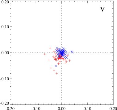
Figure 3: The distribution of star ellipticities on the complex plane for objects identified on the V image. The “plus” signs represent the uncorrected ellipticities, while the “multiply” signs represent the ellipticities corrected for the PSF. Similar plots are obtained for the other pass-bands. Note that all the points are localized near the origin of the plane, i.e. the correction is very small for FORS images.

Table 2: The number of detections obtained in the four bands. The final number of lensing galaxies used for each band is given by the last line (“Relevant galaxies”).

	Bands
Objects	B	V	R	I
Total detections	7969	7969	7969	7969
“Good” detections	6369	6315	6213	5395
Stars	66	60	76	89
Galaxies	3042	3429	3584	3178
Cluster members	253	267	269	265
Background galaxies	2750	3125	3281	2879
Relevant galaxies	1709	1844	2004	1715
CNOC galaxies	81 (58 cluster galaxies)

4.3 Identification of cluster members

Figure 4: Color-color diagram for the cluster. The open circles represent galaxies assumed to belong to the cluster; the filled circles represent galaxies with measured redshift in the range $0.29$–$0.32$; the dots are the other galaxies; crosses are residual galaxies with $R<21.5$ (see Fig. 5).

Figure 5: Color-magnitude diagram for the cluster. Symbols are as in Fig. 4.

The deep multicolor photometry provided by the FORS observations, in combination with a large number of spectroscopic redshifts on MS1008 available from the CNOC survey (Yee et al. 1998), allows the cluster galaxies to be effectively separated from the foreground and background galaxy population. Of the 81 galaxies with measured redshifts in the FORS field, there are 58 cluster galaxies with $0.29<z<0.32$, which lie along a distinctive “finger” of galaxies in the color-color plot (Fig. 4). This clump in the $V-I$ vs. $B-R$ includes most of the reddest early type galaxies in the cluster (with $V-I\approx 1.8$), as well as bluer cluster members, which are not simply distinguishable in a color-magnitude plot. Fewer late type cluster galaxies extend into a region dominated by foreground and background galaxies (filled dots with $V-I<1.4$). Thus, we are confident that the “finger tip” in Fig. 4 encompasses the majority of the cluster galaxies (254), 23% of which are spectroscopic members.

The color-mag diagram in Fig. 5 shows the same selected objects, mostly lying along the cluster red sequence. A further magnitude cut is shown, flagging all the remaining objects brighter than $R=21.5$ as likely cluster or foreground galaxies (crosses in Fig. 4 and 5). Approximately 3000 objects were thus selected as “background galaxies”.

4.4 Determination of the Shear

For gravitational lensing analyses, there have been several investigations to determine the optimal method for measuring galaxy shapes, correcting for non-gravitational shape distortions, and calibrating the gravitational shear estimates from the galaxy shape data (e.g., KSB; Luppino & Kaiser 1997; Kuijken 1999; Kaiser 2000). For ground based data, the standard approach adopted in most of the literature follows the KSB formalism to correct for PSF anisotropies and the Luppino/Kaiser (LK) algorithm for calibrating losses due to seeing and pixelization. We adopted this procedure, which, qualitatively, determines the shear map correcting for the isotropic and anisotropic part of the PSF, using a set of high $S/N$ stars in the field.

Having adopted the method for determining the shear, there are still several technical issues in the implementation of the algorithm that can introduce a bias into the results. As an attempt to minimize such effects (which we describe in more detail below), we performed a double-blind lensing analysis: two of the authors did independent, complete shear analyses, using custom designed software implementations, and somewhat different estimators to calibrate the effects of seeing and PSF anisotropies. The final results from both studies were in agreement, we thus present the results from only one implementation below. The second approach is described in the Appendix.

Defining $\epsilon^{\mathrm{s}}$ to be the unlensed, source ellipticity, we write the observed ellipticity as

$$\epsilon_{i}\simeq\epsilon^{\mathrm{s}}_{i}+P^{\gamma}_{ij}\gamma_{j}+P^{\mathrm{sm}}_{ij}p_{j}\;,$$ (4)

where we have used the Einstein convention on repeated indexes. This equation simply states that, to the first order in $\gamma$ (weak lensing limit), the observed ellipticity depends linearly on the shear $\gamma$. The quantity $P^{\gamma}$ is called pre-seeing shear polarizability, and is given by

$$P^{\gamma}_{ij}=P^{\mathrm{sh}}_{ij}-P^{\mathrm{sm}}_{ij}\left\langle\frac{P^{\mathrm{sh}}_{kk}}{P^{\mathrm{sm}}_{kk}}\right\rangle_{*}\;.$$ (5)

Here $P^{\mathrm{sh}}$ and $P^{\mathrm{sm}}$ are, respectively, the post-seeing shear polarizability and the smear polarizability; both quantity are calculated by IMCAT using the object quadrupole moments. The symbol $\langle\,\cdot\,\rangle_{*}$ indicates that the average is taken over the stars. We refer to Luppino & Kaiser (1997) for further details.

The above relation was applied as follows. We calculated for each detected star the quantity $P^{\mathrm{sh}}_{kk}/P^{\mathrm{sm}}_{kk}$, and fitted the derived values with a second order polynomial. The quantity $P^{\mathrm{sh}}_{kk}/P^{\mathrm{sm}}_{kk}$ gives information on the isotropic part of the PSF, and, as expected, we noticed little variation of this quantity across the field.

The anisotropic part of the PSF was obtained in a simple way by applying Eq. (4) to our set of stars. For stars, $\gamma=0$ (because there is no lensing effect), and $\epsilon^{\mathrm{s}}=0$ (images of stars would be perfectly round without PSF anisotropies). In conclusion, we have $p=(P^{\mathrm{sm}})^{-1}\epsilon$. As before, in order to obtain a smooth map of the anisotropies, we have fitted the $p$ with a second order polynomial, $p(\@vec{\theta})$, which is used in Eq. (4) to perform the correction. Figure 2 shows the fitted polynomial $p(\@vec{\theta})$ in the V band; the plots of the original and corrected ellipticities of stars are given in Fig. 3 (the plots for the other bands are very similar).

The determination of the shear map was handled with special care. First, galaxies characterized by a small size, a low value of the detection significance $\nu$, or a small $P^{\gamma}$ have been excluded from the catalog. For these galaxies errors on the determination of the shape parameters are quite large; moreover, they are significantly affected by the isotropic part of the PSF and thus they do not contribute to the lensing signal but only introduce noise. For the remaining galaxies we have adopted a weighted median defined in the following way. For each galaxy, we have evaluated an “individual shear estimator” given by

$$\gamma_{ij}^{(n)}=\bigl{\langle}\bigl{(}P^{\gamma(n)}\bigr{)}^{-1}_{iji^{\prime}j^{\prime}}\bigl{(}\chi_{i^{\prime}j^{\prime}}^{\mathrm{obs}(n)}-P^{\mathrm{sm}(n)}_{i^{\prime}j^{\prime}i^{\prime\prime}j^{\prime\prime}}p_{i^{\prime\prime}j^{\prime\prime}}\bigr{)}\bigr{\rangle}\;,$$ (6)

Then we assign, for each point $\@vec{\theta}$ of the field of observation $\Omega$, a weight $W^{(n)}(\@vec{\theta})=W(\@vec{\theta},\@vec{\theta}^{(n)})$ to each galaxy. Finally, we evaluate for each point $\@vec{\theta}$ of the field a weighted median of both $\gamma_{1}(\@vec{\theta})$ and $\gamma_{2}(\@vec{\theta})$. [The weighted median $\tilde{x}$ of a set of $N$ real values $x_{n}$ with weights $w_{n}$ is defined as the number such that the sum of weights on $n$ such that values $x_{n}<\tilde{x}$ is equal to the sum of weights on $n$ such that $x_{n}>\tilde{x}$. In other words, we must have

$$\sum_{n}w_{n}\mathop{\operator@font sgn}(x_{n}-\tilde{x})=0\;,$$ (7)

where $\mathop{\operator@font sgn}(x)=x/|x|$ is the function “sign” defined to be zero for $x=0$. Since in general the condition (7) cannot be exactly satisfied, a linear interpolation is used.] Alternatively, one could use a simple weighted average. Simulations, however, have shown that the median behaves much better. This is due essentially to a small number of galaxies with very poor shape determinations. In such a situation, clearly, the average is not a robust shear estimator, while the median is. As an alternative solution, one could use a suitable supplementary weight to take into account the (estimated) error on the determination of the shape parameters of each galaxy. This solution is not easy to implement because it is not always obvious if the shape of a galaxy has been measured correctly or not. Moreover, the use of supplementary weights require a fine tuning of the weighting method and this clearly leads to some arbitrariness on the reconstruction. We note that a straightforward application of the mean (standard practice in the literature) instead of the median introduces in the reconstructed shear map spurious “substructures” (i.e. secondary maxima). This is merely due to small, faint sources for which the measurement of the ellipticity is unreliable.

For the reconstructions shown below the weight $W(\@vec{\theta},\@vec{\theta}^{\prime})$ has been implemented using a Gaussian of argument $\|\@vec{\theta}-\@vec{\theta}^{\prime}\|$ and scale length $\sigma_{W}=30^{\prime\prime}$ ($\@vec{\theta}^{\prime}$ is the galaxy position). As explained by Lombardi & Bertin (1998a, 1998b), the measured shear map has noise properties that strictly depend on the weight function used. In particular, we obviously cannot expect to detect on the shear map details smaller than the characteristic scale of the spatial weight function. For the reconstructions shown here we used a Gaussian spatial weight function with a scale length $\sigma_{W}$.

4.5 Cluster mass

The dimensionless projected mass map, $\kappa(\@vec{\theta})$, was obtained using an optimized reconstruction algorithm (Seitz & Schneider 1996; Lombardi & Bertin 1998b; Lombardi 2000).

Along with $\kappa(\@vec{\theta})$, we also calculated $\sigma_{\kappa}(\@vec{\theta})$, an estimate of the error on the reconstructed mass distribution. As described in Lombardi & Bertin (1998b), this estimate takes into account the intrinsic statistical error of weak lensing reconstructions, basically proportional to $\bigl{\langle}|\epsilon^{\mathrm{s}}|^{2}\bigr{\rangle}$. We stress that $\sigma_{\kappa}(\@vec{\theta})$ is a local estimate of the error; correlation on the scale of the weighting function is expected on the reconstructed map.

In order to obtain the cluster mass in physical units we need to estimate the redshift distribution $p(z)$ of the background galaxies for each passband.

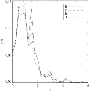
Figure 6: The redshift distribution $p(z)$ of the background galaxies in the B, V, R, and I filters derived by resampling the catalog of photometric redshift in the HDF-N.

A statistical estimate of $p(z)$ in each magnitude bin can be obtained by resampling the catalogue of photometric redshifts of Fernández-Soto et al. (1999) in the Hubble Deep Field North (HDF-N). The redshift distribution of the HDF-N derived from photometric methods is believed to be fairly reliable, given the large number of spectroscopic redshifts available in the field and the good photometric accuracy of the HDF-N images. The drawback in using the HDF-N as a reference field is of course that, for such a small field, $p(z)$ might not be representative. However, this is currently one of the few fields from which $p(z)$ can be estimated down to our magnitude limits in an empirical fashion, without resorting to galaxy evolution models for $N(z,m)$. In our analysis, we assumed that the redshift distribution of background field galaxies, as a function of magnitude, matches the one in the HDF-N. We neglected the magnification bias, i.e. the brightening of the background galaxies due to gravitational lensing, which should not be substantial in MS1008 given the lack of prominent strong lensing features.

If $N_{\mathrm{b}}(i)$ is the observed number of background galaxies in our image, in the $i$-th magnitude bin, and $N$ the total number of galaxies detected in the image, we can write

$$p(z)=\sum_{i}\frac{N_{\mathrm{b}}(i)}{N}p_{\mathrm{ref}}(z;i)\;.$$ (8)

Here $p_{\mathrm{ref}}(z;i)$ is the redshift distribution in the reference field, in the $i$-th magnitude bin, which can be written as

$$p_{\mathrm{ref}}(z;i)=\frac{1}{N_{\mathrm{ref}}(i)}\sum_{n}\delta\bigl{(}z-z^{(n)}\bigr{)}\;.$$ (9)

$N_{\mathrm{ref}}(i)$ is the total number of galaxies in the reference field in the $i$-th magnitude bin, and $z^{(n)}$ is the (photometric) redshift of the $n$-th galaxy in the reference field (the sum running on all galaxies $n$ found in a given magnitude bin).

Figure 6 shows the redshift distribution for the background galaxies, $p(z)$, derived with this method. A comparison of the observed number counts for our field with those in HDF-N is given in Fig. 7. The thick solid histogram represents the number counts of background galaxies, $N_{\mathrm{b}}(i)$. The overall number counts (thin solid histogram) clearly shows the excess at bright magnitudes due to cluster galaxies. The number counts of HDF-N galaxies with photometric redshifts (dashed curve) represent $N_{\mathrm{ref}}(i)$ in the above notation.

The knowledge of $p(z;i)\equiv p_{\mathrm{ref}}(z;i)$ for the background galaxies allows us to evaluate the projected mass distribution with an optimized method, which has the advantage of minimizing the errors on the mass distribution by properly weighting the contribution of each magnitude bin to the density $\Sigma(\@vec{\theta})$.

For each magnitude bin $i$, we can define an effective critical density as $\Sigma(z_{\mathrm{eff},i})=\bigl{\langle}\Sigma^{-1}_{\mathrm{c}}(z)\bigr{\rangle}^{-1}$, where the average is evaluated using the redshift probability distribution $p(z;i)$ (bins of $1$ magnitude were used). By using a weight proportional to $1/\Sigma_{\mathrm{c}}^{2}(z_{\mathrm{eff},i})$ in the average of Eq. (6), we take into account the fact that the lensing signal measured for galaxies in the bin $i$ decreases as the effective critical density increases.

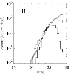
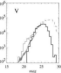
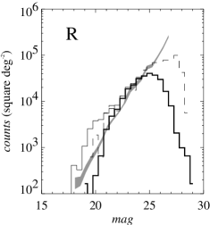
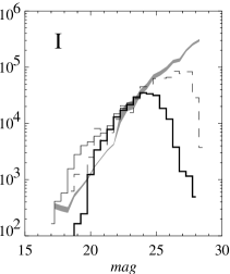
Figure 7: Observed number counts (solid line) for the galaxies in the four bands. The upper and lower solid lines correspond, respectively, to the number counts of all galaxies in the FORS field and those identified as background galaxies. We have superimposed (dashed line) the number counts of the photometric redshift catalog in the HDF-N reference field (Fernández-Soto et al. 1999). The shaded areas are number counts (with statistical errors) from the literature (Arnouts et al. 1997; Williams et al. 1996).

It is well known that the so-called mass-sheet invariance ultimately limits the accuracy in the determination of the total mass of the cluster, so that only a lower limit is strictly provided by the weak lensing analysis.

A popular method to remove the mass-sheet degeneracy is to assume that the cluster mass density vanishes at large distance from the cluster center. In doing this, we computed the radial profile of the mass map (see below) and set the minimum of this profile to zero. In this way, we almost certainly underestimate the mass density because the field of view is not large enough to include distant regions of the cluster. We also note that taking the minimum of the two-dimensional mass map is generally more risky. In fact, because of the noise, the measured mass map is not bound to be positive everywhere; on the other hand, the expected noise in the radial profile is significantly smaller (see shaded area in Fig. 11) and can be ignored for the purpose of removing the sheet degeneracy.

Another method which is often used is to assume some particular model for the projected cluster mass distribution, and to remove the sheet degeneracy by requiring that the observed mass matches the model. In the case of a singular isothermal sphere the correction to perform for the measured integral radial profile can be written explicitly. If the mass-sheet degeneracy in the observed radial profile $M_{\mathrm{obs}}(r)$ has been removed by assuming that the mass vanishes at a given radius, $r_{\mathrm{ap}}$, i.e. by setting $\bigl{\langle}\kappa(r_{\mathrm{ap}})\bigr{\rangle}=0$, then the corrected mass profile $M_{\mathrm{corr}}(r)$ is given by

$$M_{\mathrm{corr}}(r)=\frac{r+r_{\mathrm{ap}}}{r_{\mathrm{ap}}}M_{\mathrm{obs}}(r)\;.$$ (10)

Note, in particular, that when $r=r_{\mathrm{ap}}$ the mass is underestimated by a factor $2$. In our mass estimates we have used both techniques described above.

4.5.1 Projected mass distribution and radial profiles

The mass maps obtained in the four filters are shown in Fig. 8 in physical units. The average mass map (i.e., the arithmetic mean of the four independent mass maps) is also shown in Fig. 9, superimposed on the V band image of the cluster. The peak of the projected mass appears to be displaced $\sim\!30\arcsec$ north of the cD galaxy. A significant extension of the core to the north is also apparent. We should emphasize that, although the mass reconstruction is performed independently in the four images, the shear maps are not completely independent because we basically are using the same set of galaxies. In other words, we expect that the error on the averaged mass map is smaller than the error in the single bands (because we are reducing errors on the ellipticities measurements), but by a factor less than two (because we use the same galaxies).

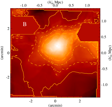
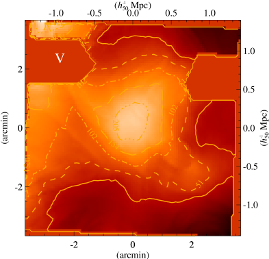
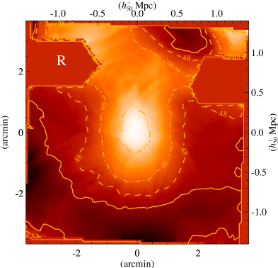
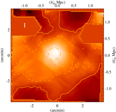
Figure 8: The mass distribution obtained from the four bands in units of $\mbox{M}_{\odot}\ h_{50}\mbox{ pc}^{-2}$. The solid line represent the contour of zero mass density. Top Left: B band; Top Right: V band; Bottom Left: R band; Bottom Right: I band.

Figure 9: The mass distribution, obtained by simply averaging the mass maps in figure 8, superimposed on the V image of MS1008. Dashed contours are labeled in units of $\mbox{M}_{\odot}\ h_{50}\mbox{ pc}^{-2}$. Solid contours correspond to zero mass density. The two blank regions on the top correspond to two bright stars masked out during the observations.

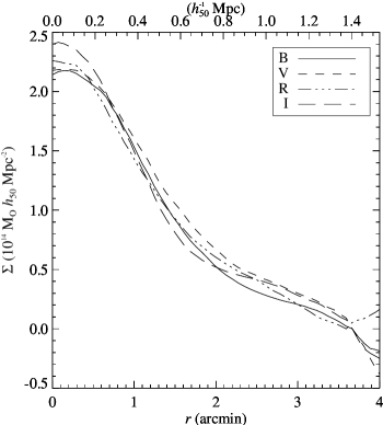
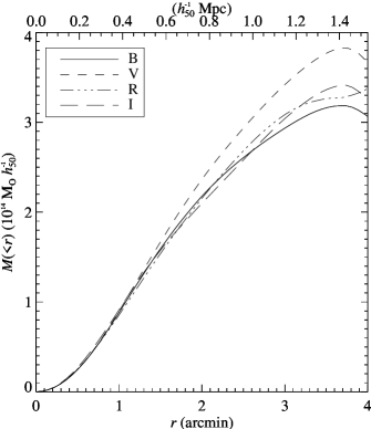
Figure 10: The radial profile (left) and the cumulative radial profile (right) of the mass distributions obtained in the four bands.

The radial profiles shown in Fig. 10 were obtained by averaging the mass distributions on annuli of increasing radii. The same center was used for all bands, corresponding to the maximum of the lensing signal.

The azimuthal average was weighted taking into account the local estimate of the error for the lens mass distribution, which depends on the local number of galaxies and on the smoothing function used. The use of a weighted average is crucial at larger radii, where two large regions are masked out. The variance $\sigma_{\kappa}^{2}(\@vec{\theta})$ was also used to estimate the errors on the radial profiles. These errors should be taken with caution, since different points of the mass profile are correlated. The differential radial profiles (Fig. 10, left) are in excellent agreement with each other, and their scatter is smaller than $5\%$. This can also be taken as a rough estimate of the error in the mass density. The cluster mass as function of radius can be read off the cumulative radial profile in Fig. 10 (right panel). In order to make these cumulative mass profiles we have broken the mass-sheet degeneracy by assuming, for each passband, that the (differential) radial profile vanishes at large radii (more precisely, at $r=3^{\prime}\,40^{\prime\prime}$, corresponding to our field of view). A comparison of different determinations of $M(<r)$ in the four passbands also gives a quantitative estimate of the systematics involved in the measurement of the total mass, in particular those associated with the way the mass-sheet degeneracy has been removed (which is responsible for the larger scatter observed in the cumulative profiles with respect to the differential radial profiles). For example, the mass out to $1h_{50}^{-1}$ Mpc is in the range $(2.7\div 3.0)10^{14}\mbox{ M}_{\odot}$, i.e. $\sim\!10\%$.

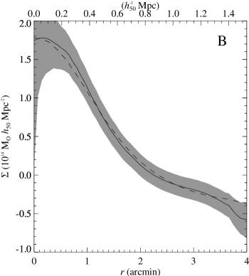
Figure 11: The radial mass profile obtained in the B filter with the errors band. The dashed curve is the result of a fit with a smoothed isothermal sphere. Very similar results are obtained for the other filters.

The radial mass profiles can also be fitted with a softened isothermal model (e.g Schneider et al. 1992). This model is characterized by the core radius $r_{\mathrm{c}}$ and the central density $\Sigma_{0}$; the projected mass distribution is then

$$\Sigma(\@vec{\theta})=\Sigma_{0}\frac{1+\|\@vec{\theta}/r_{\mathrm{c}}\|^{2}/2}{\bigl{(}1+\|\@vec{\theta}/r_{\mathrm{c}}\|^{2}\bigr{)}^{3/2}}\;.$$ (11)

Only the central $3\arcmin$ of each profile were fitted with a smoothed version of the model Eq. (11), with the same smoothing length as the one used for the shear map (see Lombardi & Bertin 1998b for a discussion the relationship between the smoothing scale used and the resulting mass map). The results of this fit are shown in Fig. 11 and summarized in Table 3. Note that the total mass within $1$ Mpc obtained from the fit is roughly the double of the mass assuming that the radial profile vanishes at large radii. This discrepancy is related to the mass-sheet degeneracy and clearly represents a serious limitation for a “total” mass estimate. We stress in particular that the correction to be applied to the “detected” mass in order to obtain the total mass strongly depends on the radial profile assumed for the cluster (the correction is exactly $2$ for a singular isothermal sphere, see Eq. (10)).

Table 3: Best fit parameters obtained in the B band.

Parameter	Value
$r_{\mathrm{c}}$ (arcsec)	$35$	arcsec
$\Sigma_{0}$	$265$	$\mbox{M}_{\odot}\ h_{50}\mbox{ pc}^{-2}$
1D velocity dispersion	$850$	$\mbox{km s}^{-1}$
Mass($r<1$ Mpc) (fit)	$5.3\times 10^{14}$	$h_{50}^{-1}\mbox{ M}_{\odot}$
Mass($r<1$ Mpc) (direct)	$2.6\times 10^{14}$	$h_{50}^{-1}\mbox{ M}_{\odot}$

4.5.2 Integrals of the shear

An alternative method to evaluate the radial profile is to use integrals of the shear (Fahlmann et al. 1994; Squires & Kaiser 1996). In particular, for a point located at polar coordinates $(r;\varphi)$ we define the tangential shear as $\gamma_{\mathrm{t}}=-(\gamma_{1}\cos 2\varphi+\gamma_{2}\sin 2\varphi)$. An estimator of the mass profile is given by

$$\zeta(\theta_{1}) = \langle\kappa\rangle(\theta_{1})-\langle\kappa\rangle(\theta_{1},\theta_{2})$$ (12)

$$= \frac{1}{\pi(1-\theta_{1}^{2}/\theta_{2}^{2})}\int_{\theta_{1}}^{\theta_{2}}\!\!\mathrm{d}r\int_{0}^{2\pi}\frac{\gamma_{\mathrm{t}}(r;\varphi)}{r}\,\mathrm{d}\varphi\;,$$

which measures the mean dimensionless mass density $\langle\kappa\rangle(\theta_{1})$ inside a disk of radius $\theta_{1}$ relative to $\langle\kappa\rangle(\theta_{1},\theta_{2})$, the mean in an annulus of radii $\theta_{1}$ and $\theta_{2}$.

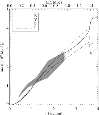
Figure 12: The (differential) mass profile estimator $\zeta$ (left) and its integral, $Z=M(<r)$ (right), for the four passbands. The shaded are shows the result from the weak lensing analysis with a different method (see text).

We show $\zeta(\theta_{1})$ in Fig. 12 for each passband; we used $\theta_{2}=3\arcmin\,40\arcsec$ which defines the edge of the images. The associated integral mass estimator, i.e. the quantity

$$Z(\theta_{1})=\Sigma_{\mathrm{c}}\pi\zeta(\theta_{1},\theta_{2})\theta_{1}^{2}\;,$$ (13)

is shown in Fig. 12. In Fig. 12 we also show in gray the same estimate as obtained independently by one of us (G. Squires) using a slightly different technique (see Appendix).

5 Mass profile from the virial analysis

The analysis of the internal dynamics of MS1008, as traced by its member galaxies, has already been discussed in the literature by the CNOC collaboration. The internal (line-of-sight) velocity dispersion for this cluster was originally measured by Carlberg et al. (1996), who found $\sigma_{v}=(1054\pm 107)\mbox{ km s}^{-1}$, based on the explicit background subtraction of the interloper contamination. More recently, Borgani et al. (2000) consistently found $\sigma_{v}=(1042\pm 110)\mbox{km s}^{-1}$, based on the completely different method for removing interlopers, as described by Girardi et al. (1998, G98 hereafter). Carlberg et al. (1996) also estimated $M_{200}\simeq 2\cdot 10^{15}\mbox{ M}_{\odot}$ for the mass within the radius $r_{200}\simeq 2.9\,h_{50}^{-1}\mbox{ Mpc}$, which is defined as the radius encompassing an average overdensity of $200$ (all the scales from the original papers have been suitably converted to those appropriate for the reference cosmological model assumed in our analysis). Lewis et al. (1999) estimated the mass within a radius $r\simeq 0.8\,h_{50}^{-1}\mbox{ Mpc}$ from ROSAT HRI X-ray data and found $M_{\mathrm{X}}\simeq 3.6\cdot 10^{14}h_{50}^{-1}\mbox{ M}_{\odot}$. They also found this value to be consistent with that obtained by extrapolating to this smaller radius the virial mass estimate at $r_{200}$ with the NFW-like (Navarro et al. 1996) profile, fitted by Carlberg et al. (1997) for the average density profiles of member galaxies for CNOC clusters.

Here, we use the galaxy data (redshift and positions) as provided by Yee et al. (1998) to determine the mass-profile of MS1008 from the virial analysis. The procedure of the selection of member galaxies is the same of G98. In addition, we also reject emission line galaxies, since they are believed not to be fair tracers of the cluster internal dynamics (e.g., Biviano et al. 1997). From G98 we also adopt the procedure for estimating the velocity dispersion $\sigma_{v}$ and the virial mass $M_{\mathrm{vir}}$, for which we provide here only a short description. As for the velocity dispersion, we find $\sigma_{v}=1033^{+115}_{-105}$ km s^-1, thus very close to previous estimates.

In the case of a spherical system and under the assumption that mass follows galaxy distribution, it is possible to show (e.g., Limber & Mathews 1960; The & White 1986) that

$$M_{\mathrm{vir}}=\frac{3\pi}{2}\frac{\sigma_{v}^{2}R_{\mathrm{PV}}}{G}-C\;.$$ (14)

Here $C$ is a term of surface pressure correction, which takes into account the fact that the radial component of the velocity dispersion does not vanish within the observational aperture radius (Carlberg et al. 1997). In the following, we assume a $20\%$ correction at the virialization scale, which is typical for nearby and CNOC clusters (G98; Carlberg et al. 1996). The value of the projected virial radius $R_{\mathrm{PV}}$ depends on the relative (projected) positions of member galaxies within the sampled cluster region.

Equation (14) provides a reliable estimate of the virial mass only if galaxy redshifts are available over the whole virialized region of the cluster. Unfortunately this is not the case for MS1008 which is sampled only within about half of the virialized region (cf. Carlberg et al. 1996). While this is not a serious problem for the estimate of $\sigma_{v}$, whose profile flattens well within the aperture radius (Borgani et al. 2000), it may represent a limitation for $R_{PV}$, whose value increases with increasing clustercentric distance. However, at each radius, an estimate of $R_{\mathrm{PV}}$ can be obtained by assuming a shape for the density profile. For instance, G98 estimated $R_{\mathrm{PV}}$ by assuming a King-like profile,

$$\rho(r)\propto\frac{1}{\bigl{[}1+(r/r_{\mathrm{c}})^{2}\bigr{]}^{\alpha}}\;,$$ (15)

with core radius $r_{\mathrm{c}}\simeq 0.1\mbox{ Mpc}$ and shape $\alpha\simeq 1.2$ [cf. their Eq. (13)], which is the best fit to the average galaxy density profile for an extended sample of local clusters. They also verified this estimate of $R_{PV}$ to be reliable for clusters sampled out to the virialization scale. In this way, we find a total virial mass which fully agrees with that given by Carlberg et al. (1996). Diamonds in Fig. 13 show the projected mass profile obtained from the King-like profile of Eq. (15).

Figure 13 also shows with the triangles the projected mass profiles obtained by scaling the original CNOC estimate with the NFW-like profile fitted by Carlberg et al. (1997). Since no definitive conclusion has been reached at present about the most appropriate profile describing the cluster galaxy distribution (see, e.g., Merritt & Tremblay 1994; Adami et al. 1998), we prefer here to show the results for both such profiles. Althouh the two virial mass determinations coincide on scales comparable to the cluster virialized regions, the choice for the density profile affects the mass reconstruction at small radii.

As a remarkable result, we find an almost perfect concordance between our weak lensing mass and the $X$-ray mass by Lewis et al. (1999). We stress that the weak lensing profiles shown in Fig. 13 have been calculated by assuming a singular isothermal sphere for the cluster mass distribution (we recall that this assumption is important when removing the mass-sheet degeneracy). As for the comparison with the virial mass reconstruction, a fairly good agreement is found at least for $r\raise-2.0pt\hbox{\hbox to0.0pt{\hbox{$\sim$}\hss}\raise 5.0pt\hbox{$>$}\ }0.4h_{50}^{-1}$ Mpc, the virial mass being only slightly larger (at about 1$\sigma$ confidence level) than that provided by the weak lensing reconstruction. The difference becomes significant only at smaller radii, where, however, both the virial and the lensing masses become more uncertain.

These results indicate that the weak lensing mass mass reconstruction do provide results which agrees with other methods, based on the assumption of dynamical equilibrium, at least in cases when high-quality imaging data are available for a fairly relaxed cluster, like MS1008 (see also Allen 1998).

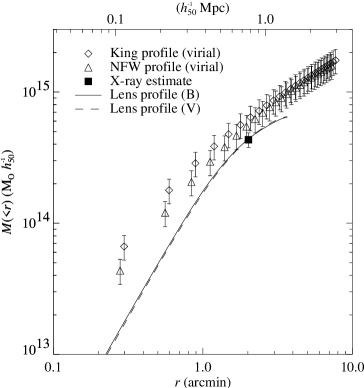
Figure 13: Comparison of different projected mass estimates. Diamonds indicate results based on the virial mass from the present analysis, rescaled with the King-like density profile of Eq. (15). Triangles are for the virial mass by Carlberg et al. (1996), rescaled with the NFW-like profile. Errorbars are $1\sigma$ uncertainties propagated from the statistical errors in the $\sigma_{v}$ estimate. The solid square is obtained by projecting the $X$-ray mass of Lewis et al. (1999), under the assumptions of spherical symmetry and NFW-like profile. The two curves are the mass profiles derived from weak lensing in two different bands.

6 Mass to light ratio

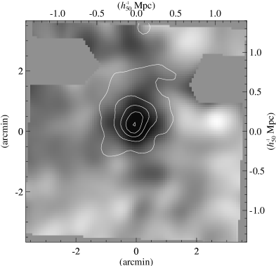
Figure 14: Left: Light distribution of MS1008 (gray scale) with overlaid mass contours, as in Fig. 8. Dots represent galaxies selected as cluster members on the basis of their color (filled dots) or redshift (crossed dots). Right: The ROSAT HRI X-ray contours overlaid on the weak lensing mass distribution (gray scale).

To evaluate the mass to light ratio, we constructed a smoothed map of the light distribution in the B band, using a Gaussian kernel with the same scale as the one used for the shear map. The light density distribution is shown in Fig. 14, with overlaid mass contours, and the cluster galaxies used in our analysis. Galaxy fluxes were measured with the SExtractor package (Bertin & Arnouts 1996), which ensures better object deblending in the cluster core with respect to IMCAT.

Luminosities were computed by assuming a k-correction of $0.7$ magnitude in V band (Fukugita et al. 1995), appropriate for ellipticals which dominate the cluster galaxy population. Luminosity evolution of early type galaxies can be neglected at this low redshift. In our cosmological model the distance modulus is $\mathit{DM}=5\log\bigl{[}D(z_{\mathrm{d}})(1+z_{\mathrm{d}})^{2}/10\mbox{ pc}\bigr{]}=41.77-5\log h_{50}$. The resulting rest-frame V-band luminosity summed over all the cluster galaxies is $L_{\mathrm{V}}=5.6\times 10^{12}h_{50}^{-2}\mbox{ L}_{\odot}$. This estimate includes galaxies as faint as $M_{*}-4$, hence the correction for incompleteness should be negligible. Carlberg et al. found $L_{\mathrm{200}}=8.8\times 10^{12}h_{50}^{-2}\mbox{ L}_{\odot}$ $(q_{0}=0.1)$ in the Gunn r band, at $r=R_{\mathrm{200}}\simeq 2.3h_{50}^{-1}\mbox{ Mpc}$. Using $(V-R)_{\mathrm{Ell}}=0.9$ and $(r-R)_{\mathrm{Ell}}=0.3$, our estimate translates to $L_{\mathrm{Gunnr}}\simeq 8.4\times 10^{12}h_{50}^{-2}\mbox{ L}_{\odot}$ at $r\simeq 1.4h_{50}^{-1}\mbox{ Mpc}$ for $q_{0}=0.1$; hence it is in very good agreement with $L_{\mathrm{200}}$ estimated by Carlberg et al.

Figure 14 clearly shows that, as commonly observed in clusters (e.g. Clowe et al. 1998), the light roughly traces the mass. The NE elongated morphology, clearly visible in the smoothed light distribution, is also shared by the intra-cluster gas, as visible in Fig. 14, which shows the ROSAT-HRI X-ray contours overlaid on the mass map (grey scale). Interestingly, the X-ray centroid is also displaced $15\arcsec$ North of the cD, i.e. nearly coincident with the peak of the weak lensing signal. The X-ray HRI data are not deep enough to probe the outer regions of the cluster. We also find some evidence for a drop of $M/L$ in the center possibly due to the presence of the over-luminous cD galaxy.

In order to properly take into account the sheet degeneracy in the evaluation of the mass-to-light ratio, we used an estimator similar to $\zeta$ for the light distribution:

$$\zeta_{\mathrm{V}}(\theta_{1})=\langle L_{\mathrm{V}}\rangle(\theta_{1})-\langle L_{\mathrm{V}}\rangle(\theta_{2})\;,$$ (16)

where $\langle L_{\mathrm{V}}\rangle(\theta)$ is V band luminosity averaged over a disk of radius $\theta$. Thus, $\zeta(\theta_{1})/\zeta_{\mathrm{V}}(\theta_{1})$ yields an unbiased estimate of the mass-to-light ratio (assuming that the light traces the mass).

Using this method we obtained $M/L_{\mathrm{V}}=95\,h_{50}\mbox{ M}_{\odot}/\mbox{L}_{\odot}$ within a radius of $3^{\prime}$, which compares favorably with the value found by Hoekstra et al. (1998), $M/L_{\mathrm{V}}=(90\pm 13)h_{50}\mathrm{M}_{\odot}/\mbox{L}_{\odot}$, for the CL 1358$+$62, with redshift ($z=0.33$) and X-ray luminosity ($L_{\mathrm{X}}[0.3-3.5\,\rm{keV}]=5.5\times 10^{44}h_{50}^{-2}\mbox{erg s}^{-1}$) very similar to MS1008.

7 Conclusions

We have studied the weak lensing mass distribution of the cluster MS1008 using multicolor imaging data obtained during the Science Verification of FORS1 on the VLT. The depth, angular resolution, and image quality across the entire field of view make these images a rare and ideal dataset for weak lensing analysis. In addition, the information on radial velocities of a large set of cluster galaxies provided by the CNOC survey allows the mass of this cluster to be derived with dynamical methods and compared with that reconstructed from the weak lensing. These combined datasets allowed us to conduct a detailed study of the systematic effects involved in cluster mass estimates.

We have found PSF distortions of FORS1 to be moderate and hence easily removed with a low order polynomial fit. The B through I multicolor information, as well as the redshift information from the CNOC catalog, have allowed us to efficiently separate the background galaxies from the cluster and foreground populations. Approximately 8000 objects have been detected, corresponding to $200\mbox{ sources arcmin}^{-2}$. Further selection lead to approximatively $1700$ background galaxies with high signal-to-noise ratio which have been used for the determination of lensing shear field. We have detected a weak lensing signal out to $r\simeq 1.2h_{50}^{-1}\mbox{ Mpc}$. The projected mass within $1h^{-1}_{50}\mbox{ Mpc}$ is measured in the range $(2.5\div 3.2)10^{14}h_{50}^{-1}\mbox{ M}_{\odot}$ in the four filters, with typical statistical errors (deriving from uncertainties in galaxy ellipticities) of 5% .

We have discussed the impact of systematics in the weak lensing reconstruction of the mass distribution in physical units, which can be summarized as follows. The removal of the mass-sheet degeneracy is inevitably model-dependent, inducing mass variations of $\sim\!15\%$ at $r\approx 1h^{-1}_{50}\mbox{ Mpc}$. [Note that the estimate of this error is difficult and somewhat arbitrary since the error clearly depend on the “range” of possible models allowed. As a result, the estimate of the total error, given below, is also bound to be inaccurate. We stress, however, that a similar problem exists for X-ray or virial mass estimate (cf., e.g., the different predictions using King-like or NFW profiles if Fig. 13).] By polluting the background galaxy population with a significant fraction of cluster galaxies, the total mass is biased low by $\raise-2.0pt\hbox{\hbox to0.0pt{\hbox{$\sim$}\hss}\raise 5.0pt\hbox{$<$}\ }5\%$. However, different selections of background galaxies, as well as edge effects due to masked portions of the images, do affect the morphology of the shear maps. We have not found any evidence for a substructure of the cluster core; this in part is due to lack of resolution in the mass reconstruction, set by the smoothing scale used. However, we have found the central region of the cluster to be elongated NS, with some evidence of a displacement of the projected mass peak respect to the cD galaxy, similarly to the X-ray emission. Cosmic variance is expected to affect the assumed redshift distribution of the background field galaxies, and hence the derived cluster mass. From a comparison between the Hubble Deep Field North and South, cosmic variance would introduce a systematic error of approximatively $10\%$ in the mass. This can also be taken as a rough estimate of the error due to cosmic variance. Note also the main contribution to this error is from large scale structures rather than from Poisson noise in the HDF-N and in our field. In other words, a simple error estimate which assumes that galaxies are uncorrelated would lead to an underestimate of the error. Altogether, the cluster light distribution traces the mass distribution remarkably well. We have measured a mass-to-light ratio of $M/L_{\mathrm{V}}=(95\pm 22)\,h_{50}\mbox{ M}_{\odot}/\mbox{L}_{\odot}$ at radii $\geq 0.5h_{50}^{-1}$ Mpc.

We have also compared the weak lensing mass profile with that derived from a virial analysis of the CNOC redshift data, as well as with the X-ray mass. The mass derived from X-ray observations (Lewis et al. 1999) is found in excellent agreement with our weak lensing determination at $r\simeq 0.8h^{-1}_{50}\mbox{ Mpc}$. Different approaches to estimate the cluster mass at the virialization scale produce very similar results. At scales $0.1\,\raise-2.0pt\hbox{\hbox to0.0pt{\hbox{$\sim$}\hss}\raise 5.0pt\hbox{$<$}\ }h_{50}r\,\raise-2.0pt\hbox{\hbox to0.0pt{\hbox{$\sim$}\hss}\raise 5.0pt\hbox{$<$}\ }1$ Mpc, lensing and virial mass determinations can be compared. The virial mass reconstruction at these small radii critically depends on the assumed density profile. Using a King-like profile describing the galaxy distribution of local clusters (G98; cf. also Eq. (15)), we have obtained a mass which is more than $2\sigma$ away from the X-ray and weak-lensing mass. Assuming instead a NFW profile, as fitted by Carlberg et al. (1997) to CNOC clusters, a much better agreement is obtained over the entire overlapping region. Note that the discrepancy at small radii ($r<1^{\prime}$) between lensing and virial estimate can be explained by recalling that the lensing determination is affected by a Gaussian smoothing of $30^{\prime\prime}$, as well as a departure from the weak lensing approximation. The former effect leads to underestimate the mass in the core, while the latter will generally bias the central mass high. Both effects clearly vanish at large radii. In addition, we notice that the weak lensing data alone cannot discriminate between different mass profiles (e.g. NFW versus isothermal model).

This analysis shows that the combination of depth and good imaging quality provided by VLT/FORS allows us to obtain high $S/N$ mass maps via optimized weak lensing reconstruction methods. On the other hand, these data have the virtue of revealing important systematic errors in weak lensing analyses. We find that the mass-sheet degeneracy dominates the budget of systematic errors and ultimately makes mass measurements via weak lensing model dependent.

The results obtained here are, at a first look, in good agreement with the mass reconstruction performed by Athreya et al. (2000). However, a detailed analysis of their study reveals that a different recipe to remove the mass-sheet degeneracy was used. Specifically, they set to zero the mass at large radii ($3\hbox{$.\!\!^{\prime}$}2$–$3\hbox{$.\!\!^{\prime}$}6$). Had they used our (model-dependent) method to break the mass-sheet degeneracy, their estimate would have been a factor of two higher. Therefore, there is a discrepancy of the same factor between the two analysis which, at present, we are unable to explain.

8 Acknowledgments

The authors would like to thank the UT1 Science Verification team at ESO for the preparation of this unique data set and its release to the community. We are particularly grateful to the VLT/UT1 Commissioning Team for carrying out the observations. We also thank Tom Broadhurst, Tomas Erben, and Peter Schneider for useful discussions. Support for this work was provided by NASA through Hubble Fellowship Grant No. HF-01114.01-98A from the Space Telescope Science Institute, which is operated by the Association of Universities for Research in Astronomy, Incorporated, under NASA Contract NAS5-26555.

Appendix A Alternative Shear Analysis

In the second analysis of the data, we followed the procedure used by Hoekstra et al. (1998). The anisotropic part of the PSF is removed on an object-by-object basis by correcting each object’s ellipticity via

$$e_{\alpha}\to e_{\alpha}-{P_{\alpha\beta}^{\rm sm}\over P_{\beta\beta}^{\rm sm}*}e_{\beta}*,$$ (17)

where starred quantities refer to parameters measured for stellar images. In this analysis, we calculated the stellar ellipticities and polarizability employing a matched radius for the Gaussian weight function as for the object in question. We fit a second order polynomial to account for spatial variations in the PSF.

We next determine the shear from the anisotropy-corrected galaxy polarizations. Both the (now effectively isotropic) PSF, and the circular weight function, tend to make objects rounder. These effects may be corrected for using the ‘pre-seeing shear polarizability’

$$P^{\gamma}=P^{sh}-P_{*}^{sh}/P_{*}^{sm}\times P^{sm}$$ (18)

introduced by Luppino & Kaiser (1997), where the $*$ subscript again refers to quantities determined from the objects classified as stars.

Operationally, to determine $\langle P^{\gamma}\rangle$, we split the faint galaxy catalogs into six bins based on size $r_{g}$, with spacing $dr_{g}=0.25$ pixels. We reject galaxies with very large, small, or negative values of $P^{sh}=(P^{sh}_{11}+P^{sh}_{22})/2$, and $P^{sm}=(P^{sm}_{11}+P^{sm}_{22})/2$ (the off-diagonal terms typically being very small). The rationale for this cut is that the calculation of the shear and smear polarizabilities for these objects failed, typically either because the objects themselves were very faint and near the detection threshold, or due to the presence of very nearby object contaminating the aperture over which the calculations were performed.

In each $r_{g}$ bin, we calculate the median galaxy polarizabilities, $P^{sh}$ and $P^{sm}$, and reanalyze the stellar catalog, resetting the value of the stellar $r_{g}$ to the bin size, and analyzing with a Gaussian with scale $r_{g}$ and an aperture three times this radius.

We finally estimate the shear for each object using

$$\gamma_{\alpha}=\frac{e_{\alpha}}{\langle P^{\gamma}\rangle}.$$ (19)

References

- (1) Adami C., Mazure A., Katgert P., Biviano A., 1998, A&A 336, 63
- (2) Allen S.W., 1998, MNRAS 296, 392
- (3) Appenzeller I. et al., 1998, The messanger 94, 1
- (4) Arnouts S. et al., 1997, A&AS 124, 163
- (5) Athreya R., Mellier Y., Van Waerbeke L., Fort B., Pello R., Dantel-Fort M., 2000, preprint astro-ph/9909518
- (6) Bertin E., Arnouts S., 1996, A&AS 117, 393
- (7) Biviano A., Katgert P., Mazure A., Moles M., den Hartog R., Perea J., Focardi P., 1997, A&A, 321, 84
- (8) Boehringer H., Tanaka Y., Mushotzky R.F., Ikebe Y., Hattori M., 1998, A&A 334, 789
- (9) Borgani S., Girardi M., Carlberg R.G., Yee H.K.C., Ellingson E., 1999, ApJ 527, 561
- (10) Broadhurst, T.J., Taylor, A.N., and Peacock, J.A., 1995, ApJ 438, 49
- (11) Carlberg R.G. et al., 1996, ApJ 462, 32
- (12) Carlberg R.G., Yee H.K.C., Ellingson E., 1997, ApJ 478, 462
- (13) Clowe D., Luppino G.A., Kaiser N., Henry J.P., Gioia I.M., 1998, ApJ 497, L61
- (14) Fahlman G., Kaiser N., Squires G., Woords D., 1994, ApJ 437, 56
- (15) Fernández-Soto A., Lanzetta K.M, Yahil A., 1999, ApJ in press
- (16) Fruchter A.S., Hook R.N., 1997, in “Applications of Digital Image Processing XX,” ed. A. Tescher, Proc. S.P.I.E. vol. 3164, 120
- (17) Fukugita M., Shimasaku K., Ichikawa T., 1995, PASP 107, 945
- (18) Girardi M., Giuricin G., Mardirossian F., Mezzetti M., Boschin W., 1998, ApJ 505, 74 (G98)
- (19) Gioia I.M., Luppino G.A., 1994, ApJS 94, 583
- (20) Hoekstra H., Franx M., Kuijken K., Squires G., 1998, ApJ 504, 636
- (21) Kaiser N., 2000, ApJ 537, 555
- (22) Kaiser N., Squires G., 1993, ApJ 404, 441
- (23) Kaiser N., Squires G., Broadhurst T., 1995, ApJ 449, 460
- (24) Kuijken, K. 1999, A&A, 352, 355
- (25) Lewis A.D., Ellingson E., Morris S.L., Carlberg R.G., 1999, ApJ 517, 587
- (26) Limber D.N., Mathews, W.G., 1960, ApJ 132, 286
- (27) Lombardi M., 2000, “Statistical Lensing,” PhD Thesis, Scuola Normale Superiore, Pisa
- (28) Lombardi M., Bertin G., 1998a, A&A 330, 791
- (29) Lombardi M., Bertin G., 1998b, A&A 335, 1
- (30) Lombardi M., Bertin G., 1999, A&A 348, 38
- (31) Luppino G.A., Kaiser N., 1997, ApJ 475, 20
- (32) Mayen C., Soucail G., 2000, submitted to A&A, preprint astro-ph/0003332
- (33) Mellier Y., 1999, Annual Review of Astronomy and Astrophysiscs 37, 127
- (34) Merritt D., Tremblay B., 1994, AJ 108, 514
- (35) Navarro J.F., Frenk C.S., White S.D.M., 1996, ApJ 462, 563
- (36) Nonino M. et al., 1999, A&AS 137, 51
- (37) Renzini, 1999, The ESO Messenger, 96, 12
- (38) Schneider P., Elhers J., Falco E.E., 1992, “Gravitational Lenses,” Springer-Verlag, Berlin
- (39) Seitz S., Schneider P., 1996, A&A 305, 383
- (40) Seitz C., Schneider P., 1997, A&A 318, 687
- (41) Squires G., Kaiser N., 1996, ApJ 473, 65
- (42) Tyson J.A., Valdes F., Jarvis J.F., Mills A.P., 1984, ApJ 281, L59
- (43) The L.S., White S.D.M., 1986, AJ 92, 1248
- (44) Williams R. E., et al. 1996, AJ, 112, 1335
- (45) Wu X.P., Chiueh T., Fang L., Xue Y.J., 1998, MNRAS 301, 861
- (46) Yee H.K.C., Ellingson E., Morris S.L., Abraham R.G., Carlberg R.G., 1998, ApJS 116, 211