UV Spectropolarimetry of Narrow-line Radio Galaxies

Abstract

We present the results of UV spectropolarimetry ($\lambda_{\rm rest}\simeq 2000-3000$Å) and far-UV spectroscopy ($\lambda_{\rm rest}\simeq 1500-2000$Å) of two low-redshift narrow-line radio galaxies (NLRGs) taken with the Faint Object Spectrograph onboard the Hubble Space Telescope (HST). Spectropolarimetry of several NLRGs has shown that, by the presence of broad permitted lines in polarized flux spectrum, they have hidden quasars seen through scattered light. Imaging polarimetry has shown that NLRGs including our targets often have large scattering regions of a few kpc to $\gtrsim 10$ kpc scale. This has posed a problem about the nature of the scatterers in these radio galaxies. Their polarized continuum has the spectral index similar to or no bluer than that of quasars, which favors electrons as the dominant scattering particles. The large scattering region size, however, favors dust scattering, because of its higher scattering efficiency compared to electrons.

In this paper, we investigate the polarized flux spectrum over a wide wavelength range, combining our UV data with previous optical/infrared polarimetry data. We infer that the scattering would be often caused by opaque dust clouds in the NLRGs and this would be a part of the reason for the apparently grey scattering. In the high-redshift radio galaxies, these opaque clouds could be the proto-galactic subunits inferred to be seen in the HST images. However, we still cannot rule out the possibility of electron scattering, which could imply the existence of a large gas mass surrounding these radio galaxies.

1 Introduction

At least some part of the population of narrow-line radio galaxies (NLRGs) are believed to harbor quasars in their central region, hidden from direct view. This has been demonstrated by polarimetric observations of these radio galaxies. The observations have shown that the radiation from some of these NLRGs is linearly polarized with the E-vector perpendicular to the radio-jet axis. Also the permitted lines are broad in the polarized flux spectra (Antonucci, Hurt, & Kinney, 1994; Young et al., 1996a; Ogle et al., 1997; Tran, Cohen, & Goodrich, 1995; Young et al., 1998; Cohen et al., 1999), the same as in Seyfert 2 galaxies (Antonucci & Miller, 1985; Tran, Miller, & Kay, 1992; Kay, 1994; Tran, 1995). In some cases, the broad components are discernable in total flux, but highly polarized and of low equivalent width.

The polarization degree often goes higher in the UV than in the optical due to the lower dilution by the unpolarized star light from the host galaxies. Therefore optical, rest-UV polarimetric observations of high-redshift radio galaxies have been done extensively (Cimatti et al., 1993; di Serego Alighieri, Cimatti, & Fosbury, 1994; di Serego Alighieri et al., 1996; Cimatti et al., 1996; Dey et al., 1996; Cimatti et al., 1997, 1998b; Tran et al., 1998). The imaging polarimetry has shown that the rest-UV image is typically elongated along the radio axis, and polarized perpendicular to this elongation (di Serego Alighieri, Cimatti, & Fosbury, 1993; Tran et al., 1998). Recently, this has been also domonstrated by UV imaging polarimetry of nearby radio galaxies (Hurt et al., 1999). Thus, all these facts fit well into the Unified Model of radio-loud quasars and radio galaxies (Barthel, 1989). The scattered light, together with the anisotropic nuclear radiation along the radio axis, has provided the explanation of at least some part of the alignment between the UV morphology and radio jet structure in $1\lesssim z\lesssim 2$ galaxies (called the alignment effect; di Serego Alighieri et al. 1989; see McCarthy 1993 for a review). In the two $z\sim 4$ galaxies observed, however, the aligned light is unpolarized starlight (4C41.17, Dey et al. 1997; 6C1909+722, Dey 1998).

While the scattering origin for much of the UV radiation has now been proven in several NLRGs, the nature of the scattering agents, i.e. hot/warm electrons and/or dust grains, still remains to be debated. The imaging polarimetry and long-slit polarimetry have revealed that the size of the scattering region in some NLRGs is of a few kpc to $\gtrsim$ 10 kpc scale (Cimatti et al., 1996; Dey et al., 1996; Tran et al., 1998; Hurt et al., 1999). This is one or more orders of magnitude larger than found in Seyfert galaxies (e.g. Capetti et al. 1995). This large size implies a rather enormous mass for the scattering gas in the NLRGs if the scatterers are electrons (di Serego Alighieri, Cimatti, & Fosbury, 1994; Cimatti et al., 1996; Dey et al., 1996). Therefore dust grains are preferred a priori to be the scattering agent, because of their much better scattering efficiency (i.e., larger scattering cross section per unit gas mass).

To address the nature of the scattering regions and environment around the hidden quasars in the radio galaxies, we need a wide wavelength coverage for the polarized flux distribution. In this paper, we present UV spectropolarimetry of low-redshift narrow-line radio galaxies obtained by the Hubble Space Telescope (HST). Combining the data with other optical/IR polarimetric data from the literature, we seek the general characteristics of the observed scattering regions. In §2, we describe our observation and data reduction process, and the results are presented in §3. We discuss the nature of the scattering region in §4, and summarize our conclusions in §5. We adopt $H_{0}=50$ km/sec/Mpc and $q_{0}=0.5$ throughout this paper.

2 Observation and Data Reduction

Three low-redshift NLRGs 3C234, 3C321 and 3C327 ($z\sim 0.1-0.2$) were observed with the Faint Object Spectrograph (FOS) onboard HST after the installation of COSTAR. We have used its spectropolarimetry mode with the grating G270H on the BLUE detector to observe $\lambda\lambda 2200-3300$Å region at $\sim$ 2.1Å per diode. We also have taken (non-polarimetric) spectroscopy data with G190H on the RED detector to observe the far-UV region $\lambda\lambda 1600-2300$Å at $\sim$ 1.4Å per diode. For these two wavelength regions, the RED detector has a higher sensitivity than the BLUE detector, but we used the BLUE detector for the former observation because of lower geomagnetically induced image motion and lower instrumental polarization. The data are summarized in Table 1. The targets were acquired using the 3-stage PEAKUP procedure of the FOS. From the target acquistion data, we have estimated the location of our observing aperture ($0.^{\prime\prime}86$ diameter) to the accuracy of $\sim 0.^{\prime\prime}2$, using the HST/FOC images (Hurt et al., 1999). The results are shown in Figures 1$\sim$3. Unfortunately, we missed the brightest region for 3C321.

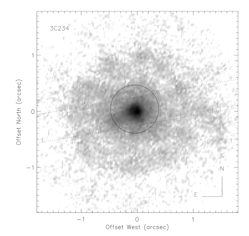
Figure 1: The location of the FOS observing aperture ($0.^{\prime\prime}86$ diameter) for 3C234 is indicated by a circle. The greyscale image is an $I$ image in log scale from the FOC imaging polarimetry data (Hurt et al., 1999). The region between the two dotted lines indicates the region extracted for calculating the polarized flux distribution in §3. Note that the FOC image was taken before the COSTAR installation, while our FOS spectra were taken after the installation. The image has not been deconvolved.

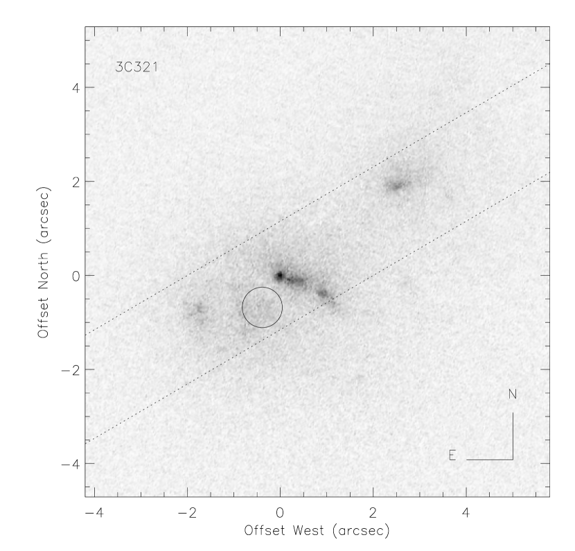
Figure 2: The same as Fig.1, but for 3C321. The image is in linear scale, and has not been deconvolved.

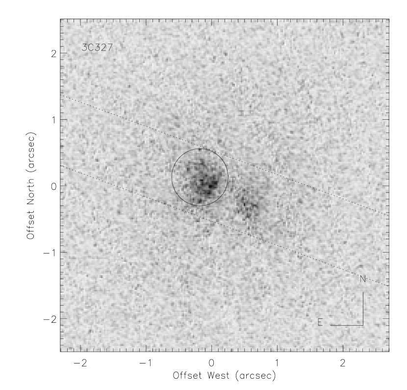
Figure 3: The same as Fig.1, but for 3C327. The image is in linear scale, and has not been deconvolved.

The data were calibrated in a standard way, as described in the HST Data Handbook (1997). The calibration procedures are (1) correction for dead diodes, (2) background subtraction, (3) flat-field correction, (4) wavelength calibration, (5) conversion to absolute flux. Several pixels with unusual noise are excluded by comparing several exposures with the same configuration. For the G270H/BLUE spectra, we have adjusted the zero point of the wavelength (Rosa, Kerber, & Keyes, 1998). The heliocentric radial velocity correction was applied. To obtain the Stokes parameters from the calibrated flux dataset, we have generated our own script on IDL described briefly below. For this process, we did not use the standard software in STSDAS because of its inadequate handling of the spectropolarimetric data.

The FOS spectropolarimetry technique is very similar to that in ground-based instruments. The waveplate is used with a Wollaston prism, which splits a beam into ordinary and extraordinary rays. These o-ray and e-ray are observerd almost simultaneously (10 seconds in turn). Spectra are taken with the waveplate rotated by 22.°5 interval. We obtained our spectra with four different waveplate positions. The signal to noise ratio was not good enough to determine Stokes $V$ parameters with this four-position observation. This prevented us from correcting for the instrumental polarization induced by COSTAR, since this correction needs the circular polarization information. However, the effect is expected to be small ($\sim 1$% level uncertainty in polarization degree for our wavelength range; Storrs et al. 1998) compared to our relatively large statistical errors in polarization. Therefore we calculated the Stokes parameters $I$, $Q$, and $U$ (after allowing for the wavelength shift between o-ray and e-ray; Storrs et al. 1998) simply from the relations

$$(1-\cos\delta)Q = J^{o}_{0}-J^{o}_{45}+J^{e}_{45}-J^{e}_{0}$$

$$(1-\cos\delta)U = J^{o}_{67.5}-J^{o}_{22.5}+J^{e}_{22.5}-J^{e}_{67.5}$$

$$I = \frac{1}{4}(J^{o}_{0}+J^{e}_{0}+J^{o}_{45}+J^{e}_{45}$$ (1)

$$+J^{o}_{22.5}+J^{e}_{22.5}+J^{o}_{67.5}+J^{e}_{67.5})$$

assuming that the circular polarization is zero (for each intensity $J$, subscripts denote waveplate positions and superscripts denote o-ray/e-ray; $\delta$ is the retardation of the waveplate). We did not perform any correction for the COSTAR-induced instrumental polarization. The circular polarization in our objects is expected to be very small. After this, the Q and U are corrected for the variation of waveplate axis over the wavelength and converted from instrumental coordinates to sky coordinates (Allen & Smith, 1992).

We have first subtracted the background using the canonical values from the standard calibration pipeline. The FOS background counts basically correlate with the geomagnetic position of the HST at the time of the observation (Hayes & Lindler, 1996). The canonical background values in the pipeline are derived from this information, but there could be some residual counts. For the far-UV observation with G190H, there are unilluminated pixels and we have used them for the scattered light subtraction and additional background subtraction adjustment. With G270H (spectropolarimetric data), however, there are no unilluminated pixels available. We found that with the canonical background subtraction, the blue side of the G270H Stokes $I$ spectra did not match well with the red side of the G190H spectra for each object. Therefore we scaled the canonical background for G270H spectra to match with the G190H spectra. The scaling factors were found to be 1.35, 1.38, and 1.45, for 3C234, 3C321, and 3C327, respectively. These scaling values are rather large, suggesting that the canonical backgrounds were systematically underestimated for these observations. The scattered light in our G270H spectra is expected to be small since our objects are rather red (Rosa, 1994). We have confirmed the color of our objects by calculating the optical flux in our observing aperture using the archival WFPC2/F702W images. The geomagnetic image motion could affect the spectra, but in our case this effect is expected to be small because our observing aperture was $0.^{\prime\prime}86$, where the height of diodes is $1.^{\prime\prime}29$ and the typical uncorrected geomagnetic motion is $0.^{\prime\prime}15$, and because real-time onboard corrections were done. Also the telescope pointing was good in our observations, judging from the available jitter data.

Note that this background scaling, or background itself, essentially does not affect the unnormalized Stokes parameters $Q$ and $U$ systematically, thus does not affect the polarized flux and position angle of polarization systematically (but affects $P$, through $I$). The $Q$ and $U$ are essentially obtained from the difference of the o-ray and e-ray [see eq.(1)], and these two rays are observed almost simultaneusly as described above. The FOS background counts originate mainly from high energy particles hitting the photocathode or detector itself, and are considered to reside equally in o-ray and e-ray spectra.

3 Results

Figures 4 $\sim$ 6 show the results of our spectropolarimetric observations. The far-UV spectra are given in Figures 7 $\sim$ 9. The errors are calculated from the statistical error of the raw counts. Due to the aperture miscentering for 3C321, we could not detect polarization for this object (Fig.5). For 3C234 and 3C327, we have detected high polarization ($10\sim 20$ % level). For these objects, the UV polarization is roughly constant over the observed UV wavelength range.

Figure 4: UV Spectropolarimetry of 3C234. From top to bottom, $I$ spectra, fractional polarization, position angle, and polarized flux are shown with 1$\sigma$ error bars. The flux unit is erg cm^-2 sec^-1 Å^-1. The position angle is in degrees. In the top panel, two $I$ spectra are shown : the upper one has the true flux, and the lower one is the true flux multiplied by 1/5. Both of $I$ spectra have been smoothed by 1 diode width (= 4 pixel). The line identifications are shown, and also note the possible bumps from the Fe II lines at around $\sim 2400$Å and $\sim 2100$Å. In other panels, the dotted lines show the averaged values over the whole observed wavelength. The polarized flux has been debiased following Simmons & Stewart (1985).

Figure 5: UV Spectropolarimetry of 3C321. From top to bottom, the $I$ spectrum (binned with 3 diodes = 12 pixels) and normalized Stokes spectra $Q/I$ and $U/I$ are shown. Note that the observing aperture missed the brightest region.

Figure 6: UV Spectropolarimetry of 3C327. The styles are the same as Fig.4, except that the $I$ spectra are binned with 2 diodes = 8 pixels.

Figure 7: Far-UV spectrum of 3C234, smoothed by 1 diode (= 4 pixel).

Figure 8: Far-UV spectrum of 3C321. Note that the observing aperture missed the brightest region.

Figure 9: Far-UV spectrum of 3C327, binned with 2 diodes (= 8 pixel).

We also show the properties of the emission lines seen in our spectra in Table 2, determined by fitting a gaussian for each line. For the line widths, the instrumental width of 1 diode has been subtracted in quadrature. For 3C234, the broad components are seen in the total flux at C IV $\lambda$1549 and C III] $\lambda$1908. For the former, there seems to be two distinct broad components with FWHM of $\sim 3000$ km sec^-1 and $\sim 20000$ km sec^-1. We show the line fitting results in Figure 10. The simultaneous fit of the continuum (power law) and several lines (gaussians) resulted in having the continuum slope of $F_{\nu}\propto\nu^{-0.85\pm 0.11}$, but this could be uncertain due to the low S/N in the short wavelength side. If the real continuum is redder as in the longer wavelengh side (see Fig.4, though note the possible Fe II contributions), the extremely broad component of the C IV line could be even broader and would have a larger flux. For the broad component in the C III] line, there might also be two components, but the smaller EW and the blend with the Si III] line prevented us to do a reliable two-component fit. For 3C327, we see broad Mg II $\lambda$2800 line in the total flux. We tentatively determined its FWHM to be $\sim 8000$ km sec^-1, although there could be contributions from broad Fe II emission lines in this region.

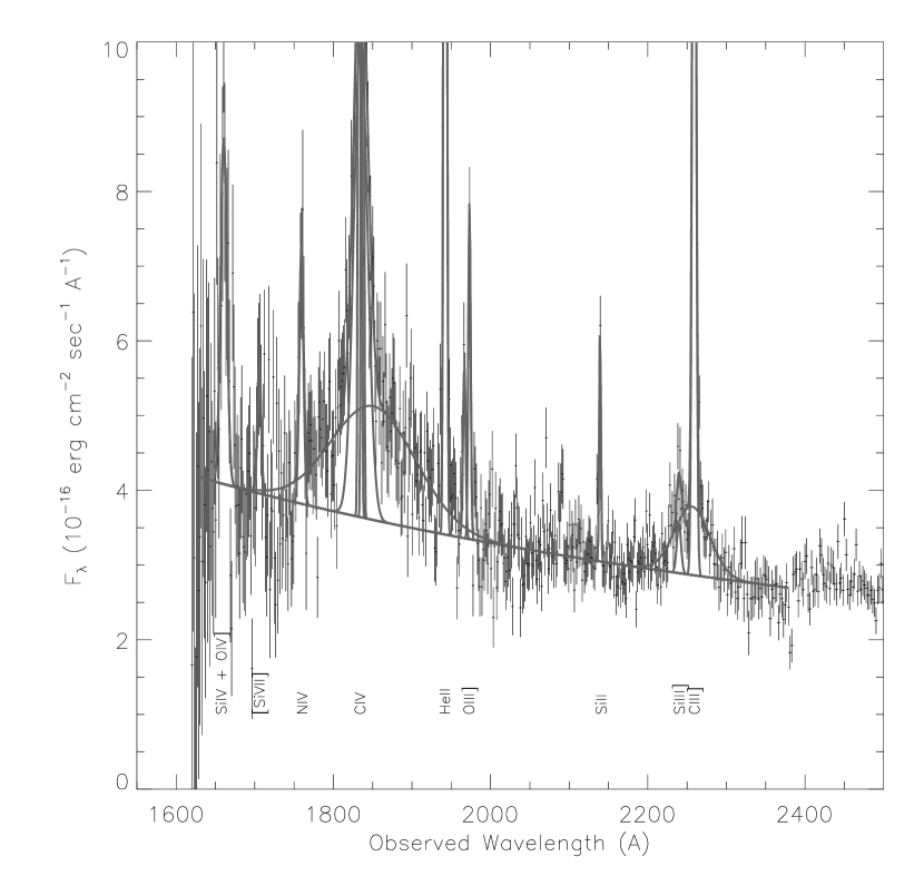
Figure 10: The line fitting result for the far-UV (G190H) spectra of 3C234. The G270H has been combined at 2280Å. Table 2 lists the fitted parameters. The simultaneous fit of the continuum and several lines indicated was implemented. The obtained continuum slope is $F_{\nu}\propto\nu^{-0.85\pm 0.11}$, but this could be uncertain due to the low S/N in the short wavelength side. If the real continuum is redder as in the longer wavelengh side, the extremely broad component of the C IV line could be even broader and would have a larger flux.

As we described in §2, we have increased the amount of the background subtraction for the spectropolarimetry data, compared to the nominal background. The background subtraction affects only $I$, and does not have an influence on $Q$ and $U$ (unnormalized Stokes parameters). The object counts are lower at shorter wavelength which have lower sensitivity, so the fraction of the background counts are larger there. Therefore, larger background subtraction results in smaller $I$ and larger $P$ at the shorter wavelength. This changes the total flux level and its spectral shape rather significantly in 3C321 and 3C327 since the background fraction in these objects was rather high. However, the overall wavelength dependence of $P$ does not change significantly compared with the relatively large error in $P$. The polarized flux is not influenced, as the $Q$ and $U$ do not change.

Table UV Spectropolarimetry of Narrow-line Radio Galaxies compares our spectropolarimetric results with the previous observations. Slight discrepancies in position angles (PAs) are possibly explained through the differences in observing aperture sizes. We show the polarization extracted at different positions and apertures from the HST UV imaging polarimetry data (Hurt et al., 1999) taken with F320W filter ($\lambda_{\rm obs}\sim 3100$Å) in Figures 11 and 12. In 3C234, the nucleus has an extension to the south east on $\sim 0.^{\prime\prime}5$ scale. (Also the nucleus seems to be slightly elongated to the north east on $\sim 0.^{\prime\prime}1$ scale. The PSF through the F320W filter is known to be elongated, but this elongation direction is different from the one seen in the nucleus.) This extension seems to be polarized differently from the nucleus, though the values for this component in Figure 11 are only suggestive since this FOC image is pre-COSTAR data. The optical imaging polarimetry data of Cohen et al. (1999) show similar PA distribution (see their Fig.5f). Our FOS observing aperture has possibly excluded some portion of the south-east component. This would explain at least partly the slight difference in PA between our FOS data and larger aperture data. For 3C327, the nucleus is double, or the image suggests the existence of two scattering cones. These two features have slightly different polarization. Our FOS aperture was centered on the brighter one, and the polarization extracted only for this feature is consistent with our FOS result. As described in Hurt et al. (1999), the exposure time for one of the polarizer images of 3C327 was uncertain, but the uncertainty is probably less than 5 seconds (R. Jedrzejewski, private communication; we adopted the same exposure time as in Hurt et al. 1999). The resulting uncertainty of the measured polarization in Figure 12 is less than the quoted statistical error. Conversely, this is supported by the agreement with our FOS result.

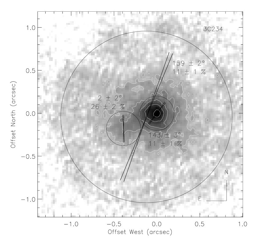
Figure 11: Imaging polarimetry of 3C234 (Hurt et al., 1999), with three different synthetic apertures. The PA and polarization are written with each aperture, together with two lines indicating the directions of PA$\pm\sigma_{\rm PA}$. The image is the same as Fig.1. Contours in percent of the peak are 5, 10, 20, 40, 80. Note that the polarization off the nucleus is only suggestive since this data set is pre-COSTAR and the influence of the central bright point-like source is hard to quantify.

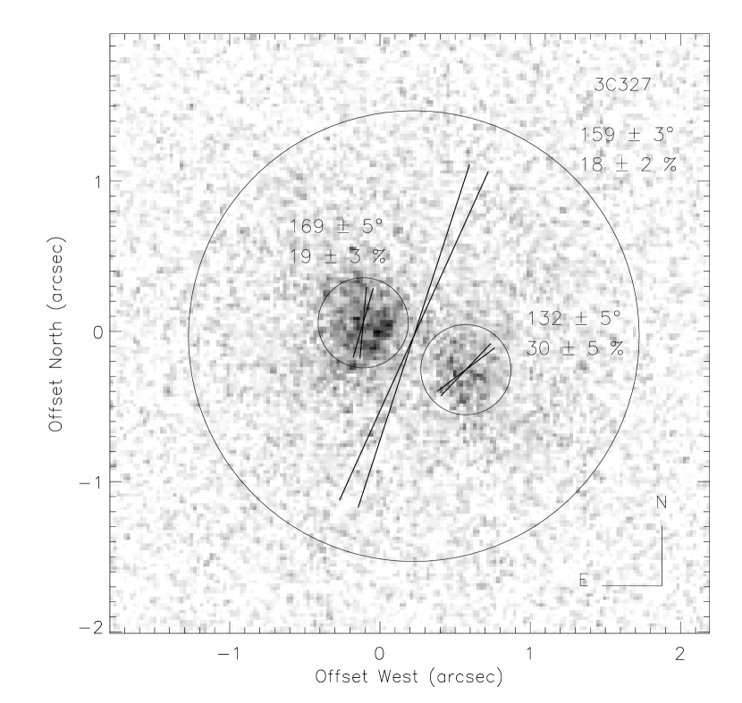
Figure 12: The same as Fig.11, but for 3C327. The image is the same as Fig.3.

From the resolved polarized flux distribution in the imaging polarimetry data, we can derive the physical extent of the scattering region. We have extracted the image with a certain width along the elongation direction for each object. The Stokes parameters $Q^{\prime}$ and $U^{\prime}$ are calculated with the polarization reference axis perpendicular to this elongation. The extracted regions (direction and width) are indicated in Figures 1$\sim$3, and we show the $Q^{\prime}$ and $U^{\prime}$ distributions in Figures 13$\sim$15. The figures indicate that the polarized fluxes from these radio galaxies are extended from a sub-arcsecond to arcsecond scale, which corresponds to a few kpc to 10kpc (though the size for 3C234 would be lower, since the imaging polarimetry data are pre-COSTAR). This is one or more orders of magnitude larger than the spatial scale of the scattering region seen in Seyfert galaxies. The sizes are summarized in Table 4.

Figure 13: Polarized flux distribution in 3C234 along the direction of PA = 100°. The extraction width is $0.^{\prime\prime}5$. See Fig.1 for the extraction window. The solid and dotted lines indicate Stokes $Q^{\prime}$ and $U^{\prime}$, respectively, with its reference axis perpendicular to PA = 100°. Note that the size of the polarized flux distribution was influenced by the aberrated central bright point-like source (pre-COSTAR data).

Figure 14: The same as Fig.13, but for 3C321 along the direction of PA = 120°and width = $2.^{\prime\prime}0$. See Fig.2 for the extraction window.

Figure 15: The same as Fig.15, but for 3C327 along the direction of PA = 70°and width = $1.^{\prime\prime}0$. See Fig.3 for the extraction window.

4 Discussion

In this section, we discuss the observed polarized flux spectra comparing these with the observed quasar continuum. We refer to the typical quasar continuum shape as $\alpha\simeq-0.3$ where $F_{\nu}\propto\nu^{\alpha}$ at $\lambda_{\rm rest}=1\sim 0.15$µm (Neugebauer et al., 1987; Francis et al., 1991; Francis, 1996). Some papers find steeper typical slopes, in part because of the apparent luminosity dependence (Mushotzky & Wandel, 1989), and sometimes because the so-called 3000Å bump is not removed. Also of course since the underlying continuum is sometimes convex, the rest wavelength intervals are important. We note that, however, even if the intrinsic optical and UV spectral shape ($\gtrsim 2000$Å) is slightly redder, such as the composite spectra of $\alpha\sim-0.7$ (Cristiani & Vio, 1990), this essentially does not affect our conclusions below. The spectral shape could be even redder at shorter wavelength (Zheng et al., 1997), but this basically is not relevant here since we mainly discuss the polarized flux of wavelength longer than $\sim 2000$Å, except for the discussion of high-redshift radio galaxies (§4.5).

4.1 The feasibility of electron scattering

Our UV spectropolarimetry shows that the continuum polarization is roughly independent of wavelength, and as we will see in §4.4, the polarized flux shape from the UV to optical is similar to or redder than the typical quasar continuum. These might suggest that the dominant scattering is being caused by electrons (plus reddening), rather than by dust grains. Its feasibility, however, is quite low. As we have seen in the previous section, the scattering regions in these radio galaxies are rather large. The previous work on the distant high-redshift NLRGs has shown that the scattering regions are even larger, $\gtrsim 10$ kpc scale (3C256 : Dey et al. 1996; 3C265 : di Serego Alighieri et al. 1996, Tran et al. 1998; 3C324 : Cimatti et al. 1996). This fact favors dust grains as the dominant scatterers. First, the scattering cross section per hydrogen atom, $\sigma$, for dust grains in the optical or UV is two or three orders of magnitude larger than Thomson scattering cross section in the interstellar medium of our Galaxy (see below for more specific values), and may not be too different in the scattering region in these radio galaxies. Dust should survive at these large scale regions, and large dust masses are observed to exist in many high-redshift radio galaxies and quasars (Dunlop et al., 1994; Chini & Krugel, 1994; Cimatti et al., 1998a). Secondly, even if the amount of dust is a few orders of magnitude less than that in our Galaxy and the electrons are to take the role as the dominant scatterers, the large sizes of the scattering region observed imply enormous masses for the scattering gas (di Serego Alighieri, Cimatti, & Fosbury, 1994; Cimatti et al., 1996; Dey et al., 1996). This argument is summarized as follows.

The scattered luminosity $L_{\nu}^{s}$ is described by, using the nuclear luminosity $L_{\nu}$,

$$L_{\nu}^{s}=\frac{L_{\nu}}{4\pi}\sigma\int\frac{n}{r^{2}}dV.$$ (2)

where $n$ is the hydrogen density, $r$ is the radial distance from the nucleus, $\sigma$ is again the scattering cross section per hydrogen atom, and $V$ is the volume. The integral is taken over the whole scattering region, assuming an optically thin case. Let us define a geometrical factor $g$ as

$$g=\frac{\int ndV}{R^{2}\int\frac{n}{r^{2}}dV}$$ (3)

where $R$ is a characteristic size for the scattering region. This factor depends on the geometry of the scattering region but is of order unity. Using this factor, we can relate the total number of hydrogen $\int ndV$ to the scattering fraction $L_{\nu}^{s}/L_{\nu}$ as

$$\frac{L_{\nu}^{s}}{L_{\nu}} \equiv \tau\Omega/4\pi$$ (4)

$$= g^{-1}\frac{\sigma}{4\pi R^{2}}\int ndV$$

Here, we rewrote the scattering fraction as $\tau\Omega/4\pi$ (which means that it corresponds to the average optical thickness of the scattering medium, $\tau$, multiplied by the covering factor of the medium with respect to the central illuminating source, $\Omega/4\pi$, but we are not assuming any particular geometry of the scattering region here). Thus the mass for the scattering gas $M_{\rm scat}$ necessary to achieve a certain scattering fraction is written as

$$M_{\rm scat}=3.8\cdot 10^{10}\left(\frac{\tau\Omega/4\pi}{0.01}\right)g\left(\frac{R}{5{\rm kpc}}\right)^{2}\left(\frac{\sigma}{\sigma_{T}}\right)^{-1}M_{\sun},$$ (5)

where $\sigma_{T}$ is the Thomson scattering cross section. Note that the gas mass surrounding the nucleus could be larger than $M_{\rm scat}$ by a factor of several or more, since we are considering only the gas illuminated by the nucleus and there should be more unilluminated gas (e.g. outside of the ionization cone).

We have adopted the value of 0.01 as a typical value for the scattering fraction $\tau\Omega/4\pi$. For our three objects, we can compare their UV luminosity with that of the quasars with the same low-redshift range and with the same radio lobe power. Those differ from our objects mainly in orientation alone according to the unified model. The UV polarized flux luminosity of our three objects is Log $PL_{\nu}$ (erg sec^-1 Hz^-1) = $27.4\sim 28.2$ at $\lambda_{\rm rest}\sim 2500$Å and their radio power at 178MHz is Log $P_{178}$ (erg sec^-1 Hz^-1 sr^-1) = $32.6\sim 33.7$, while the 3C quasars with $z\lesssim 0.3$ and with the same radio power range have Log $L_{\nu}$ = $29.0\sim 30.9$ at $\lambda_{\rm rest}=2500$Å (we have taken absolute magnitudes from Veron-Cetty & Veron 2000 and converted them with $F_{\nu}\propto\nu^{-0.3}$). If we think that the intrinsic polarization is less than $\sim$ 50%, the scattered light would be larger than the polarized flux at least by a factor of $\sim 2$. Therefore the scattering fraction 0.01 is a representative approximation. Consideration of reddening would make the scattered luminosity of these radio galaxies brighter, so would make $M_{\rm scat}$ even larger. Thus, if the scatterers are electrons $(\sigma=\sigma_{T})$, a large mass is implied. On the other hand, only a relatively small mass is necessary if the dominant scatterers are dust grains: the scattering cross section $\sigma$ for dust grain per H atom is $\sigma\sim 300\sigma_{T}$ at $V$ and $\sigma=600\sim 900\sigma_{T}$ at $\lambda=3000\sim 2000$Å in our Galaxy, assuming the column density of H atoms per $E(\bv)$ = $7.5\cdot 10^{21}$ cm^-2 (Jenkins & Savage, 1974), $A_{V}/E(\bv)=3.1$, and albedo of 0.5.

The recombination-line luminosity provides another argument, if we consider the line luminosity from the scattering region. Let us consider a simple case of a scattering region with density $n$, volume $V$, and volume filling factor $f$, so that we have the amount of gas $\int ndV\simeq nVf$ and the emission measure $\int n^{2}dV\simeq n^{2}Vf$. With the scattering region size $R$ and the amount of the gas $\int ndV$ from the above estimation [equation (5)], we can estimate the H$\alpha$ luminosity $L_{H\alpha}$ to see if we predict the right amount with a reasonable value of $f$;

$$L_{H\alpha} \simeq 4\pi j_{H\alpha}\frac{\left(\int ndV\right)^{2}}{V\cdot f}$$ (6)

$$= 4.7\cdot 10^{43}\cdot f^{-1}\cdot\left(\frac{\tau\Omega/4\pi}{0.01}\right)^{2}g^{2}$$

$$\mbox{ }\left(\frac{R}{5{\rm kpc}}\right)\left(\frac{\sigma}{\sigma_{T}}\right)^{-2}\enspace{\rm erg}~{}{\rm sec}^{-1}.$$

We simply adopted the volume of $\frac{4}{3}\pi R^{3}$, and the H$\alpha$ emissivity $j_{H\alpha}$ for $T=10^{4}$K. The density is estimated as

$$n \simeq \frac{\int ndV}{Vf}$$ (7)

$$= 2.9\left(\frac{\tau\Omega/4\pi}{0.01}\right)g\left(\frac{R}{5{\rm kpc}}\right)^{-1}$$

$$\mbox{ }\left(\frac{\sigma}{\sigma_{T}}\right)^{-1}f^{-1}\enspace{\rm cm}^{-3}.$$

For our three radio galaxies, H$\alpha$ luminosity is of the order of $10^{42}\sim 10^{43}$ erg sec^-1 (table 4). If we assume dust scattering, the observed line luminosity can be easily accomodated with a small value of $f$ ($10^{-4}\sim 10^{-5}$). The density will be of order $10^{2}$ cm^-3 in this case. On the other hand, when assuming electron scattering, to avoid the overprediction of H$\alpha$ luminosity, the volume filling factor should be close to unity, or not be too far from unity, which is quite surprising. The density will be of order 1 cm^-3 in this case.

This situation can be summarized as follows. In the electron case, for which a large amount of gas is implied, the gas has to be spread over the entire volume to have smaller density for suppressing the line emission. In the dust case, for which a smaller amount of gas is needed, the gas should be squeezed into a smaller effective volume to have higher density to get the same line emission.

Higher $T$ of $\sim 10^{7}$ K, as will be discussed in §4.4 (but not too high to avoid smearing out the scattered broad line completely), could reduce $L_{H\alpha}$ by about a few orders of magnitude. One possibility for electron scattering is a hot diffuse volume-filling gas without much line emission, possibly surrounding the narrow-line region, though this still suffers from the large mass problem.

4.2 Optically thin dust scattering

The mostly constant polarization and the polarized flux spectrum no bluer than typical quasars would lead us to consider electron scattering, but the feasibility arguments above would suggest dust grains to be the dominant scatterers. Below we attempt to summarize the property of dust scattering, for the interpretation of the polarization data of radio galaxies.

The most robust way to investigate the wavelength dependence of the scattering process is to look first at the polarized flux spectrum with a wide wavelength range, then look at the total flux spectrum considering the possible diluting components. These diluting components, such as stellar radiation and nebular continuum, usually have no influence on the polarized flux spectrum. The polarized flux from the scattering process is the product of the incident spectrum and the polarizing efficiency $\epsilon$, where $\epsilon$ is the scattering efficiency $\kappa$ times the intrinsic polarization degree $P_{0}$ which is the degree of polarization of the scattered light from the scattering process. In optically thin dust scattering, $\kappa$ is simply proportional to the scattering cross section $\sigma$ which has a rather strong wavelength dependence, and $P_{0}$ has a moderate wavelength dependence. We have to compare the product of these two with the ratio of the observed polarized flux spectrum to the typical quasar continuum shape, $\alpha\simeq-0.3$ where $F_{\nu}\propto\nu^{\alpha}$. For the optically thick case, $\kappa$ will be significantly different, which will be discussed in the next section. We focus on optically thin cases in this section.

The scattering cross section of the extreme case is the Rayleigh scattering limit where $\sigma\propto\nu^{+4}$. This is for the case of very small particles. For Galactic dust, the scattering cross section has been investigated through the observations of reflection nebulae (Witt & Gordon 2000 and references therein). It generally increases with decreasing wavelength, but its wavelength dependency changes with wavelength range, as shown in Figure 16. The scattering cross section is proportional to $\sim\nu^{+2}$ in the near IR ($\sim 2\ \micron-0.9\ \micron$) and its spectral index gets flatter with shorter wavelength. In the optical ($\sim 0.9\ \micron-0.3\ \micron$) it is roughly proportional to $\nu^{+1}$. In the UV, the extinction cross section has a bump at $\sim$ 2200Å, but this feature seems to be purely in absorption, not in scattering (Calzetti et al., 1995). This 2200Å feature is weak in the LMC (Misselt, Clayton, & Gordon 1999 and references therein), and it is absent in the star-forming bar of the SMC (Gordon & Clayton 1998 and references therein) and in starburst galaxies (Calzetti, Kinney, & Storchi-Bergmann, 1994; Gordon, Calzetti, & Witt, 1997). In this UV range ($\sim 0.3\ \micron-0.1\ \micron$), while the extinction cross section for Galactic dust generally goes up rapidly at wavelengths shorter than the bump (although it depends on the sight line: Calzetti, Clayton, & Mathis 1989), the wavelength dependence of the scattering cross section seems to become somewhat flatter with $\sim\nu^{+0.5}$, though the empirical work on the albedo at $\lambda\lesssim 2000$Å varies for different objects and thus it is still poorly understood (Witt & Gordon, 2000). For the SMC, the extinction rapidly goes up roughly with $\nu^{+1.5}$, but no empirical work on the scattering cross section exists.

Figure 16: The wavelength dependence of extinction (upper curve) and scattering (lower curve) optical depth for Galaxy (solid) and SMC (dotted). The data values are taken from Witt & Gordon (2000).

Several authors have done theoretical calculations of dust properties. In an early paper, Mathis, Rumpl, & Nordsieck (1977) inferred the composition and size distribution of the dust grains that reproduce the Galactic extinction curve. White (1979) calculated the scattering and polarization properties for this population of dust. Recently Zubko & Laor (2000) have calculated the polarization properties using updated dielectric functions. These latter two calculations suggest that the polarization of the scattered light in a single dust scattering process, $P_{0}$, is moderately wavelength-dependent. In Zubko & Laor (2000), the maximum polarization, which is achieved when the scattering angle is around 90°, is approximately flat at about 30 $\sim$ 35% (versus 100% for electron scattering) in the UV/optical region of $\sim$ 1700Å $-$ 7000Å. To longer wavelength, it goes up to $\sim 60$% at $\sim 1\ \micron$. To shorter wavelength in the far UV, it also rather rapidly increases reaching $\sim 60$% at 1000Å. The region around 2200Å would be highly uncertain because these theoretical calculations produce the 2200Å enhancement in the scattering cross section, as opposed to the observational result by Calzetti et al. (1995), though this is the only empirical result at present. At smaller or larger scattering angle, the polarization degree becomes smaller, but the overall wavelength dependence is similar. We obtain the polarizing efficiency $\epsilon$ by multiplying the scattering cross section and this polarization degree $P_{0}$. For the region of the most interest in this paper, $0.2-0.7$µm, $P_{0}$ seems to be approximately constant, so the shapes of the scattering efficiency $\kappa$ and polarizing efficiency $\epsilon$ are almost the same, and thus $\epsilon$ is proportional to roughly $\nu^{+1}$ for the Galactic dust, if there is no 2200Å bump in the scattering cross section as observed by Calzetti et al. (1995). For the SMC dust, $\epsilon$ would be roughly proportional to $\nu^{+1.5}$. For the shorter wavelenth (far-UV), $\epsilon$ would be slightly bluer, and for the longer wavelength (near-IR), it would be somewhat redder.

Some observational results actually show this blue polarizing efficiency or blue scattering efficiency. In the prototype Seyfert 2 galaxy NGC 1068, an off-nuclear knot at about $5^{\prime\prime}$ NE from the nucleus shows a blue polarized flux spectrum $\alpha\simeq+1$ where $F_{\nu}\propto\nu^{\alpha}$ ($\beta\simeq-3$ where $F_{\lambda}\propto\lambda^{\beta}$; Fig.5 in Miller, Goodrich, & Mathews 1991) in the optical region ($\lambda\lambda 3600-6400$Å). We can compare this spectrum with the polarized flux from the nuclear vicinity to obtain the polarizing efficiency, since the scatterers are considered to be electrons there. Its spectral index is $\alpha\simeq-0.5$ ($\beta\simeq-1.5$; Fig.6 in Miller et al. 1991) or $\alpha=0.0$ ($\beta=-2.0$; with a wider wavelength coverage and a narrower slit width; Tran 1995), so we obtain the polarizing efficiency in this case to be $\epsilon\propto\nu^{+1}\sim\nu^{+1.5}$. This is consistent with the general optically-thin dust scattering property. In the radio galaxy PKS2152-69 (di Serego Alighieri et al., 1988), the extranuclear cloud shows very blue scattered light, $\alpha=+3\pm 1$, which could indicate that the scattering efficiency (not the polarizing efficiency in this case) $\kappa$ is roughly proportional to $\nu^{+3\pm 1}$, assuming a typical quasar spectral index for the nuclear continuum. This could be close to the case of Rayleigh scattering, but with a rather large uncertainty. None of other radio galaxies is known to show this type of behavior.

4.3 Opaque clumpy dust clouds

What if the dust clouds are optically thick ? Generally, if we see a scattering wall or slab of dusty gas which is optically thick at all wavelength regions, the wavelength dependence of the scattering efficiency would essentially correspond to the albedo (not the scattering cross section) of the scattering medium. For Galactic dust, the albedo is observed to be mostly flat in the UV-IR wavelength regions. In this sense, its scattering efficiency curve would be rather similar to electron scattering. But in reality, we will observe the scattering region through various viewing angles, and this would cause a wavelength dependence of the scattering efficiency especially when the clouds are only moderately optically thick. Also, in the case of radio galaxies, the scattering region would not be uniformly optically thick as a whole in terms of the unification of radio galaxies and quasars, since otherwise we would not observe any quasars. The optically thick regions should be localized, i.e., the scattering region as a whole should be clumpy as actually observed in 3C321, and it is each of these clumps which could be optically thick. Then, the general property of this scattering region can be approximately derived from that of a single spherical scattering blob.

The calculation of the scattering properties of such a blob has been implemented by Code & Whitney (1995) using the Monte Carlo method. Figure 17 reproduces their result for the dust scattering with albedo = 0.5 and scattering asymmetry parameter $g$ = 0.56 (forward-throwing), which are for a representative case for UV/optical dust scattering (Witt & Gordon, 2000). The symbols in Figure 17 are the scattered flux per unit solid angle for a certain viewing angle $\psi$ (which is the scattering angle at the blob) with unit incident flux, multiplied by $4\pi$. It corresponds to the scattering fraction for a blob, integrated assuming isotropic scattering. Since the single dust scattering process is forward-throwing, the scattering dusty blob is also forward-throwing, and this is true even for the case of rather large optical thickness. (We multiplied the scattered flux by $4\pi$ to show an apparent scattering fraction, which we would infer from observations because viewing angle is usually unknown.)

Figure 17: Scattered flux from a spherical dusty blob as a function of extinction optical thickness for diameter $\tau_{b}$ and for different viewing angles (which correspond to the scattering angle at the blob), taken from Code & Whitney (1995). It is the scattered flux per unit solid angle with the incident flux being unity, multiplied by $4\pi$. Therefore it corresponds to the scattering fraction for a blob integrated over the whole solid angle assuming isotropic scattering. The squares, crosses, and triangles are for the viewing angle 30°, 90°, and 150°, respectively. The dotted lines illustrate the fits by the form of $\tau_{\rm scat}\exp(-\tau_{\rm ext}^{\rm eff})$ for small $\tau_{b}$, which fail at larger $\tau_{b}$.

When the viewing angle $\psi$ is small (forward scattering case), we will see the strong forward-scattered light through a significant amount of extinction. When viewed edge-on ($\psi\sim 90\arcdeg$), this extinction effect becomes smaller. When $\psi$ is large (backward scattering case) we will see relatively weak back-scattered light with a smaller amount of extinction, and the scattered light will be saturated with large optical thickness, just like seeing a thick wall. In all these cases, the scattered flux first increases proportionally to the increase of the scattering optical thickness of the blob (denoted here as $\tau_{\rm scat}\equiv a\tau_{b}$, where $a$ is albedo and $\tau_{b}$ is extinction optical thickness for the diameter of the blob). Then it starts to have some effective amount of extinction ($\tau_{\rm ext}^{\rm eff}$), which increases with the blob optical thickness ($\tau_{\rm ext}^{\rm eff}\propto\tau_{b}$). For relatively small blob optical thickness, the scattered flux can be approximated by $\tau_{\rm scat}\exp(-\tau_{\rm ext}^{\rm eff})$ (similar expressions have been used by other authors, e.g. Cohen et al. 1999). More specifically, the data points, say $f$, in Figure 17 for relatively small $\tau_{b}$ can be approximated by

$$f=a(2\tau_{b}/3)\cdot 4\pi\Phi(\psi,g)\cdot e^{-\tau_{\rm ext}^{\rm eff}},$$ (8)

where

$$\tau_{\rm ext}^{\rm eff}=\xi(2\tau_{b}/3).$$ (9)

The phase function $\Phi$ is given in Henyey & Greenstein (1941). The factor 2/3 added to $\tau_{b}$ represents the effective thickness of the sphere of diameter $\tau_{b}$. The factor $\xi$ corresponds to the effective fraction of extinction of the scattered light. The dotted lines in Figure 17 illustrate that we can fit the calculation results with only one parameter $\xi$ for relatively small $\tau_{b}$ (up to $\sim$ 2.0). This effective extinction fraction $\xi$ is close to unity but decreases with increasing viewing angle (the adopted values for the fit in Fig.17 are 0.9, 0.6, 0.4 for $\psi=30\arcdeg,90\arcdeg,150\arcdeg$), since we will see the light with a shorter path inside the blob for larger viewing angle.

In terms of the observations, this $\tau_{b}$ dependence of the scattered light corresponds to the wavelength dependence of the scattering efficiency since the optical thickness of the blob is proportional to $\sim\nu^{+1}$. It initially follows the form of $\tau_{b}e^{-\xi(2\tau_{b}/3)}$. However, for larger optical thickness, which corresponds to shorter wavelength observation, the scattered flux will not decrease exponentially, as illustrated in Figure 17. The fit described above fails at larger optical thickness. This is because for larger $\tau_{b}$ the effective extinction optical thickness $\tau_{\rm ext}^{\rm eff}$ does not grow proportionally to $\tau_{b}$, but instead grows slower: the parameter $\xi$ [eq.(9)] for a given viewing angle is not actually constant, but decreases with $\tau_{b}$ (we only see more foreground part of the blob where extinction is smaller). Thus, once the blob becomes opaque for the observing wavelength, its scattering efficiency becomes flat or decreases to the shorter wavelength but not exponentially. This means that the wavelength dependence of the optically-thick scattering efficiency is bluer than that of foreground screen extinction, for which we expect an exponential cut-off at the shorter wavelength.

We note that in the optically thick case with the Galactic dust, the scattering efficiency and polarizing efficiency will have some dip across the 2200Å, since Calzetti et al. (1995) showed that the albedo has a dip at the 2200Å, based on the enhancement in absorption and non-enhancement in scattering across the 2200Å feature. The scattered light (and polarized flux) will decrease around 2200Å because of this absorption enhancement. In the SMC or starburst galaxies, the 2200Å feature does not show up in the extinction, so the albedo would be flat across the 2200Å region. There would be no feature in the scattered light from such dust grains. The observations of radio galaxies are still not definitive on this issue. In our spectrum of 3C234, we do not see any feature. In the spectrum of 3C327, the feature, if it exists at all, is not clear.

4.4 Nature of the scattered light in 3C234, 3C321, and 3C327

To investigate the nature of the scatttered light for the three radio galaxies in our program, we combine our UV polarization data with the previous optical/IR polarimetry data in the literature. The HST UV imaging polarimetry is available in Hurt et al. (1999) for all three objects. The polarized flux spectra from UV to IR are shown in Figures 18, 19, and 20.

4.4.1 3C234

For 3C234, we have plotted ground-based large-aperture polarimetry data (see Table UV Spectropolarimetry of Narrow-line Radio Galaxies) and spectropolarimetry data (Tran et al. 1995). The latter is a $1^{\prime\prime}$ slit observation with the seeing $\lesssim 1^{\prime\prime}$ and thus the absolute flux is lower, so we have scaled the data to fit the large aperture data with the same wavelength regions (of course this is only meaningful if the scattering mechanism is the same). Although our UV polarized flux with the $0^{\prime\prime}.86$ aperture could be missing some part of the whole polarized flux, as indicated by the slight PA rotation (see §3), its flux level matches that from the large synthetic aperture photometry of the UV imaging polarimetry data (Hurt et al., 1999). In Figure 18, all fluxes have been corrected for the small Galactic reddening $E(\bv)=0.019$ (NED; based on Schlegel et al. 1998).

Figure 18: Total flux and polarized flux observed in the UV/optical/IR for 3C234. The FOS UV polarized flux spectrum is plotted in solid ticks with vertical error bars, and above this, the UV total flux is shown in dashed lines. The optical spectropolarimetry data (Tran et al., 1998) are plotted in dots. The optical/IR broad band data with large apertures in Table UV Spectropolarimetry of Narrow-line Radio Galaxies are shown in solid (polarized flux) and dashed (total flux) ticks with error bars. The polarized flux of Tran et al. has been scaled to match the optical large-aperture polarized flux (so the latter is almost embedded in the former and hard to see), and the total flux spectrum was also scaled by the same factor. All polarized and total fluxes have been corrected for the small Galacic reddening with $E(\bv)=0.019$.

The optical polarized flux has been found to be very red compared to the typical quasar continuum (Tran et al. 1995) : we measure the spectral index $\alpha$ ($F_{\nu}\propto\nu^{\alpha}$) between H$\alpha$ and H$\beta$ to be $\simeq-1.7$ from Tran et al. data (for $\lambda\lambda 5200-5800$Å to avoid any possible influence of broad H$\alpha$ line). Also, the Balmer decrement in the polarized flux is large (7.3; Tran et al. 1995). These facts, as well as the large Pa$\alpha$/H$\alpha$ ratio for the broad components in the total flux, have been interpreted to be due to a significant reddening of $A_{V}=2.4\sim 2.7$ (Carleton et al. 1984; Hill et al. 1996; Tran et al. 1995; we have summarized the observed slope and line ratios in Table 4.)

However, a simple screen reddening does not explain our UV polarized flux observation. The polarized flux spectrum can be fitted with a power law down to the UV, if we exclude 2600Å $<\lambda_{\rm rest}<4000$Å region to allow for the possible so-called 3000Å bump : $\alpha=-1.7\pm 0.2$ for the optical-UV from the large-aperture optical data and our UV data, and $\alpha=-1.7\pm 0.6$ for the UV only. A significant amount of dust screen (such as the one to redden the optical spectrum from $\alpha\simeq-0.3$ to $-1.7$) should absorb the UV greatly so that the resulting spectrum would have an exponential decrease toward the UV. Thus, a dust screen is unlikely to be the cause of the red continuum of 3C234.

We note that the redness of the optical continuum and Balmer decrement in the broad-line radio galaxies and radio-loud quasars have been found to have a correlation, which has been interpreted to be due to reddening (Baker, 1997). The observed values for the optical polarized flux of 3C234 actually fit into this correlation (see Fig.16 in Baker 1997). But our UV data for 3C234 is not compatible with this reddening interpretation because of the lack of a cutoff in the UV. Also, note that the reddening inferred in the quasar colors must show an exponential UV cutoff, if a dust screen is present.

If the polarized flux continuum of 3C234 is without a significant reddening, this would mean that the broad H$\alpha$ and H$\beta$ lines in 3C234 have a different reddening. The possibility of Broad lines having different reddening from continuum has been discussed by some authors (e.g. Baker 1997). Alternatively, the Balmer decrement could be intrinsically large in 3C234: the optical depth effect will make the Balmer decrement larger (e.g. Kwan and Krolik 1981). In this case, to explain the large Pa$\alpha$/H$\alpha$ ratio observed, we might have to consider a different component in the IR. We will discuss this later below.

As for the scattering mechanism in 3C234, the red, apparently no-reddening continuum suggests that an optically-thin dust scattering is not a dominant contributor. Otherwise, the incident continuum has to be redder than the observed one, which would be unlikely. On the other hand, an opaque dust scattering would explain the observation. If the viewing angle is rather small, it will make the continuum redder but without an exponential decrease, as we have seen in the previous section.

As described in §3, however, an extremely broad component with FWHM of $\sim 20000$ km sec^-1 is observed in the C IV line of our UV total flux spectrum (Fig.10), in addition to an ordinary broad component. We have inspected the H$\alpha$ region in the polarized flux spectrum of Tran et al., and tentatively identify an extremely broad component of similar width (or even broader). These extremely broad lines could be intrinsic to the broad line region of 3C234, but also could be due to scattering broadening by hot electrons with $T\sim 10^{7}$ K. Thus some part of the scattered light might be from electrons. We note that the gas mass implied for electron scattering case would be less of a problem for 3C234, because the observed scattering region is rather compact.

Now we discuss briefly the IR polarized flux. We have calculated the K band polarized flux using the polarization data at 2µm with $5.^{\prime\prime}8$ aperture (Sitko & Zhu, 1991) and total flux data with $7.^{\prime\prime}5$ aperture (Lilly, Longair & Miller, 1985). The polarization data from Young et al. (1998) is consistent with the former, but the absolute flux seems to be lower by a factor of $\sim$ 2 due to the smaller aperture ($3.^{\prime\prime}08\times 3^{\prime\prime}$) as described by them. We tentatively do not use the H band data from Brindle et al. (1990), since the H band total flux ($\sim 1360\mu$Jy) shows a rather strange dip by a factor of about 2 between the J band and K band flux (2050 $\mu$Jy and 5500 $\mu$Jy, respectively). Note, however, that there are emission line contributions in J and K bands, such as He I $\lambda$10830 and Pa$\alpha$.

Having these in mind, the observed K band polarized flux forms almost the same spectral shape as the optical ($\alpha=-1.6\pm 0.1$ over the IR to the optical). Typical quasar continua actually turn up at around 1 µm and have a steeper spectral shape in the IR with $\alpha=-1.4$ (or $-2\sim-1$; Neugebauer et al. 1987) than in the optical. Apparently, the IR continuum polarized flux of 3C234 could be consistent with no or little reddening. However, the large Pa$\alpha$/H$\alpha$ ratio would not be consistent with this. Again, the broad lines would have different reddening than the continuum, or alternatively, the large ratio might be suggesting that another polarized component is coming in in the IR, which could be highly-reddened scattered light from the inner region, or a dichroic polarization component (Young et al., 1998). Note that the PA does not change in the IR from the optical.

In summary, for the scattering mechanism in 3C234, we infer that opaque dust scattering with a rather small viewing angle might be playing a role, though some part of the scattered light could be from electrons.

The hybrid case of dust-scattered and electron-scattered light seems to be realized actually in nature. It could be the situation exactly in NGC 1068 for a large aperture $6^{\prime\prime}\times 12^{\prime\prime}$, including the NE dust knot, observed in the UV (Code et al., 1993), where the UV polarized flux is significantly influenced by the dust scattered light. In the case of Cygnus A, the polarized H$\alpha$ line is extremely broad (Ogle et al., 1997), but the Mg II line is much narrower (Antonucci, Hurt, & Kinney, 1994). Therefore, scattering agents could be different in these two wavelength regions, and electron scattering might be contributing at least at $H\alpha$, though the Galactic-reddening corrected flux ratio of these two lines could be consistent with optically-thin dust scattering (Ogle et al., 1997).

4.4.2 3C321

For 3C321 (Fig.19), we have combined the optical/IR polarization data by Young et al. (1996a) with the FOC UV imaging polarimetry data. The nucleus of 3C321 consists mainly of two components, separated by $\sim 3.^{\prime\prime}3$. The $5^{\prime\prime}$ aperture polarimetry of Young et al. (1996a) seems to be centered on the brighter, SE component. Hurt et al. (1999), however, give the integrated polarization for the whole of both two components, so we have implemented the synthetic $5^{\prime\prime}$ aperture polarimetry centered on the SE component, the result of which is shown in Table UV Spectropolarimetry of Narrow-line Radio Galaxies and Figure 19.

Figure 19: Total flux (dashed ticks) and polarized flux (solid ticks) observed for 3C321 in the near-UV/optical/IR wavelength regions are plotted with error bars. All fluxes have been corrected for the Galactic reddening with $E(\bv)=0.044$. The data are in Table UV Spectropolarimetry of Narrow-line Radio Galaxies.

The Galactic reddening is $E(\bv)=0.044$ (NED; based on Schlegel et al. 1998). The centro-symmetric pattern of the position angle distribution of the optical polarization does not seem to be disturbed by the Galactic interstellar polarization (Cohen et al., 1999; Draper, Scarrott, & Tadhunter, 1993). The spectral shape of the polarized flux with the $5^{\prime\prime}$ aperture corrected for the Galactic reddening is $\alpha=-0.1\pm 0.3$ ($\lambda_{\rm rest}=2500\sim 6500$Å). The spectropolarimetry by Tadhunter, Dickson, & Shaw (1996) shows that the optical polarized flux spectrum has $\alpha=-0.3$, and the polarized flux continuum of Young et al. (1996a) is consistent with this result. Cohen et al. (1999) have taken optical spectropolarimetric data with a slit across these two nuclei ($1^{\prime\prime}\times 17^{\prime\prime}$ extraction size), and showed that the polarized flux spectrum integrated is of $\alpha=0.0$, while the Balmer decrement seems to be not too large.

The scattering region of 3C321 is very extended, so the results of polarimetry will be different for different size and location of the apertures and seeing conditions. Nevertheless, these results suggest that, overall, the wavelength dependence of the polarizing efficiency is apparently quite flat or slightly blue in the optical to the near-UV.

What is the nature of this polarized flux ? At the central region, there is evidence for reddening in the morphology of the optical image taken by HST (see Fig.2 in Hurt et al. 1999) where a dust lane is clearly seen. Also, the narrow line components have been shown to be reddened at the central region : from H$\gamma$/H$\beta$, Tadhunter et al. (1996) obtained $A_{V}=2.9\pm 0.6$ with $1.^{\prime\prime}6$ slit; from Pa$\alpha$/H$\alpha$/H$\beta$, Hill et al. (1996) obtained $A_{V}=1.5\pm 0.3$ for the central $\sim 2.^{\prime\prime}5\times 2.^{\prime\prime}5$ region. Therefore, the polarized flux from this central region could also be reddened. The significant part of the polarized flux, however, is coming from the outer region. Using the UV imaging polarimetry data of Hurt et al. (1999), we have compared the polarized flux from the central $2.^{\prime\prime}5$ region with that from the outer region within the $5^{\prime\prime}$ diameter masking the central $2.^{\prime\prime}5$. They are found to be approximately of the same amount. Therefore, the possible explanation of the flat or slightly blue polarizing efficiency would be that the reddened polarized flux from the central $\sim 2^{\prime\prime}$ region is compensated by the blue optically-thin dust scatterered light from the outer region.

We also compared the polarized flux from the observed clumps (including the NW component) with that from the surrounding diffuse gas, and found that they have a comparable amount, though the definition of the diffuse region is somewhat arbitrary and also the data suffer from the abberation (pre-COSTAR). This polarized flux from the diffuse region would be optically-thin dust scattered light, while the polarized flux from the clumps might be opaque dust scattered light. The latter would have roughly neutral scattering efficincy if the viewing angle is close to edge-on, which would be expected from the morphology with a dust lane.

However, the possibility of electron-scattering contribution cannot be ruled out, aside from the huge mass implied if this is the case for the diffuse extended region. The spectral shape of the polarized flux is not blue enough to rule it out to be neutrally scattered light. Also, an inspection of Fig.2 of Cohen et al. (1999) possibly suggests a faint but extremely broad component at H$\alpha$ [like Cyg A (see the same Fig.2 in Cohen et al; Ogle et al 1997); or 3C234 (see previous section)].

The IR polarized flux (see Fig.19) seems to have a different component, though the S/N for the K band data is only about 3. This component could be another highly-reddened scattered component or could be a dichroic polarization component. We need more IR polarimetric observations to clarify the nature of this component.

4.4.3 3C327

The UV and near-UV radiation of 3C327 is highly polarized, while in the optical the polarization is rather low. In table UV Spectropolarimetry of Narrow-line Radio Galaxies, we list our UV data, UV imaging polarimetry data of Hurt et al. (1999), and also the large-aperture optical and IR data of Young et al. (1996b) with 3$\sigma$ upper limit for $P<2\sigma_{P}$. In Figure 20, we have plotted our UV data scaled by the ratio of the polarized flux in the large synthetic aperture data of Hurt et al. (1999) to our polarized flux with $0.^{\prime\prime}86$ aperture at $\lambda_{\rm obs}=2700\sim 3300$Å, assuming that the two regions seen in the UV image have the same polarized flux spectral shape. This scaling ratio was found to be 2.27. The U band and H band data from Young et al. (1996b) are also shown, with the latter as an upper limit. To illustrate the optical polarized flux in Figure 20, we have included optical spectropolarimetry data obtained at the Keck telescope during a cloudy night in June 1996 [$1^{\prime\prime}$ slit, 10 minutes exposure per position angle; Dey, Antonucci, & Cimatti, unpublished. Note that [O III]$\lambda$4959+5007 seems to be detected in the polarized flux, which was first suggested by di Serego Alighieri et al. (1997)]. We scaled the data to have the polarized flux at the blue end ($\sim 4700$Å) match with the 3$\sigma$ upper limit at the B band. With this scaling, the total flux is only slightly smaller ($10\sim 20$% level) than the large-aperture data.

Figure 20: Total flux (dashed ticks/lines) and polarized flux (solid ticks) observed for 3C327 in the UV/optical/IR wavelength regions. The arrow is a 3$\sigma$ upper limit. The spectra of our FOS observations have been scaled to match at $\lambda_{\rm obs}=2700\sim 3300$Å to the FOC imaging polarimetry data. The unpublished optical spectropolarimetry data (Dey et al.) are included, which is scaled to match the 3$\sigma$ upper limit of the polarized flux at B band (Young et al. 1996b ; see Table UV Spectropolarimetry of Narrow-line Radio Galaxies). All fluxes are corrected for the Galatic reddening with $E(\bv)=0.089$.

If we correct for the Galactic reddening, taking $E(\bv)=0.089$ (NED; based on Schlegel et al. 1998) and $R_{V}=3.1$, then we obtain $\alpha=+0.5\pm 0.8$ for the polarized continuum (using continuum bins only) from the UV to near-UV ($\lambda_{\rm rest}=2000\sim 3500$Å; FOS + U band data). The optical polarized flux spectrum, corrected for the Galactic reddening assuming negligible contribution from interstellar polarization, is consistent with this result at the UV, though not too constraining : the spectral index $\alpha$ is $-0.01\pm 0.94$. If we combine the UV and optical polarized flux, we obtain $\alpha=-0.01\pm 0.21$ ($\lambda_{\rm rest}=2000\sim 7500$Å), though there is uncertainty from the scaling and using the upper limit at B band (the true shape could be bluer). There could be an influence from the 3000Å bump, and in that case, the intrinsic shape would be slightly redder.

The narrow lines have been found to be reddened. From Pa$\alpha$/H$\alpha$/H$\beta$ ratios, Hill et al. (1996) obtained $A_{V}=1.2\pm 0.3$ (see Table 4 for the observed ratios). The narrow emission line region is observed to be extended (total extent of $\sim 4^{\prime\prime}$; Baum et al. 1988), though not well resolved. On the other hand, the polarized flux does not seem to show a large decrease in the shorter wavelength. Therefore, the scattering region may not be cospatial with the narrow-line region, or again, the optically-thick dust clouds with an edge-on view (as inferred from the UV morphology) could be playing a role. We emphasize, however, that the above arguments are subject to the uncertainties in the scaling factor of our UV polarized flux, and the low signal to noise of the polarization measurements.

4.5 Hidden quasars in other objects

In the high-redshift narrow-line radio galaxies with extended scattering regions (over 10kpc scale), 3C256 ($z$=1.824), 3C265 ($z$=0.811), and 3C324 ($z$=1.206), their rest-frame UV polarized flux spectral shape is similar to or rather redder than the typical quasars. For 3C256 (Dey et al., 1996), the polarized flux spectral index is $\alpha\simeq-1.1$ ($PF_{\nu}\propto\nu^{\alpha}$) for the rest wavelength range of $1400-3200$Å. For 3C265 (Tran et al., 1998), $\alpha=0$ for $\lambda_{\rm rest}=2200-4900$Å. For 3C324 (Cimatti et al., 1996), $\alpha=-2.0\sim-1.5$ for $\lambda_{\rm rest}=1800-4100$Å. The reddening for the polarized flux in these objects is still uncertain, though for the total flux of 3C256 the reddening for narrow lines is inferred to be small from the HeII line ratio (Dey et al., 1996), and for 3C324, Cimatti et al. (1996) concluded that the polarized flux spectrum is explained by electron or dust scattering only if reddening with $E(\bv)$ = 0.25 - 0.35 is assumed.

For 3C277.2 ($z$=0.763; Tran et al. 1998), there is slight evidence for an extended scattering region, and the polarized flux spectrum shape is roughly $\alpha=-0.6$ at $\lambda_{\rm rest}=2200-5000$Å, allowing for a possible 3000Å bump. In 3C356 ($z$=1.079; Cimatti et al. 1997) and 4C23.56 ($z$=2.482; Cimatti et al. 1998b), which are also high-redshift narrow-line radio galaxies, the morphology is double and one of the two components exhibits high polarization. For 3C356, $\lambda_{\rm rest}=2000-4300$Å, Cimatti et al. (1997) found that the polarized flux can be explained either by electron scattering or by dust scattering + reddening ($E(\bv)=0.05$). For 4C23.56, $\alpha$ is roughly $-1.5$ for $\lambda_{\rm rest}=1200-2600$Å, and in this far-UV range the polarization clearly goes up.

In the hyperluminous infrared galaxies, IRAS P09104+4109 ($z$=0.442), IRAS F15307+3252 ($z$=0.926), and IRAS F10214+4724 ($z$=2.286), the total flux shows only narrow lines, but the polarized flux reveals broad permitted lines. Therefore they are interpreted to harbor a QSO, which is seen in reflection. For the former two galaxies, the spectral shape of the polarized flux is again similar to that of a typical QSO (the continuum shape would not be too different from quasars; e.g. Cristiani & Vio 1990) : $\alpha=-0.5$ for IRAS P09104+4109 at $\lambda\lambda_{\rm rest}3900-5500$Å (excluding the 3000Å bump region; Hines et al. 1999; Hines & Wills 1993), and $\alpha=-0.5$ for IRAS F15307+3252 at $\lambda\lambda_{\rm rest}2200-4200$Å (Hines et al., 1995). For IRAS F10214+4724, which is a gravitationally lensed galaxy (Nguyen et al., 1999), the polarized flux is rather red: $\alpha=-1.4$ at $\lambda\lambda_{\rm rest}1200-2700$Å (Goodrich et al., 1996). For IRAS P09104+4109, the spatial polarized flux distribution has been found to be extended (a few kpc; Hines et al. 1999). Also, the extinction of the narrow lines for this galaxy is inferred to be $A_{V}=1.8\pm 0.6$ (Soifer et al., 1996).

We have summarized the spectral slopes quoted above in Figure 21. For comparison, the typical quasar spectral shape is also illustrated (see the first part of this §4 for the description and references). The comparison seems to be telling us that we observe the polarized flux spectrum similar to or redder than the quasar spectrum, but not bluer. This is why we often cannot rule out electron scattering even with the poor plausibility. Its implication is considered in the next section.

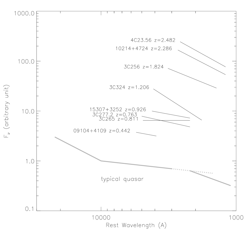
Figure 21: Illustrates rough spectral shapes of the polarized flux spectra observed in high redshift galaxies. We have put the spectra in the order of redshifts. The flux is in $F_{\nu}$, and only the relative flux in a given object is valid. A typical quasar continuum shape is also drawn in the thick line at the bottom. We adopted $\alpha=-0.3$ for the optical spectrum, where $F_{\nu}\propto\nu^{\alpha}$ (Neugebauer et al., 1987; Francis et al., 1991; Francis, 1996). The spectrum could be steeper, especially in the UV (so we made the line of $\alpha=-0.3$ dotted in the UV), as indicated by the quasar composite spectra such as Cristiani & Vio (1990) and Zheng et al. (1997). The latter far-UV shape is also illustrated in the thick line at the bottom right.

4.6 The case for opaque dust or electron scattering

As we have seen, we rarely observe scattered light bluer than the spectral shape range observed for quasars. Also, the polarized flux has never been observed to have an exponential cut-off in the shorter wavelength range so far, which suggests no simple screen reddening. Therefore, optically-thin dust scattered light would not probably be dominating the whole scattered flux in general ($\Delta\alpha=+1$ or more is expected; see §4.2). A possibility is that in a lot of cases, the significant part of the scattering dust clouds, if there is any, are probably opaque. In this case, red scattered light without an exponential decrease in the shorter wavelegth would be naturally explained.

Is it feasible that the blobs seen in radio galaxies are optically thick in the UV ? Here we do some rough estimation using equations (6) and (7) in §4.1. Note that those equations are for optically thin case, but they would be valid until the optical thickness of the blob becomes unity. We take $L_{H\alpha}=10^{43}$ erg sec^-1 for a fiducial example. Then we obtain $f\sim 10^{-5}$ [eq.(6)] assuming the cross section per H atom = 600$\sigma_{T}$ for the UV radiation. In this case, we have $n\sim 500$ cm^-3 from equation (7). On the other hand, in the HST images of high-redshift radio galaxies (Best, Longair, & Röttgering, 1997; Pentericci et al., 1999), the resolved knots in the rest-UV are of $\sim$ 1 kpc scale, and the number of knots in each object is several to $\sim$ 10. Therefore, the apparent volume filling factor of these knots in the whole scattering region ($\sim$ 10 kpc scale or more) is $10^{-2}\sim 10^{-3}$. This means that the volume filling factor inside the clump would be about $10^{-5}/10^{-2}\sim 10^{-5}/10^{-3}$. With the density of the order of $10^{2}$ cm^-3, the average column density through the clump (clump size $\times$ density $\times$ volume filling factor inside the clump) would be of the order of $10^{21}$ cm^-2. Thus, this clump will be optically thick in the UV if there is no particular dust-destroying condition. Therefore, it would be feasible to have opaque blobs.

If these knots seen in the high-redshift radio galaxies are proto-galactic subunits as inferred by Pentericci et al. (1999), these will certainly provide the actual physical origin of the opaque dusty clumps discussed here, since such subunits will have a large surface mass density. Conversely, we can estimate the lower limit for the mass of an opaque dusty clump from the size scale of the clump (diameter $2r$) and average column density through the clump ($N_{H}$) as

$$M \simeq m_{H}\pi r^{2}N_{H}$$ (10)

$$= 6\times 10^{6}\left(\frac{2r}{1{\rm kpc}}\right)^{2}\left(\frac{N_{H}}{10^{21}{\rm cm}^{-2}}\right)M_{\sun}.$$ (11)

The possibility for electron scattering, however, still cannot be ruled out, aside from the large mass problem. The extremely broad component ($\sim$20000 km sec^-1 or more), seen in the C IV line of 3C234 or possibly in the H$\alpha$ lines of 3C234 and 3C321, might suggest the scattering broadening by hot electrons ($\sim 10^{7}$ K). If the spatial distribution of these electrons is really extended to $\sim$ 10kpc scale and thus have a huge mass, this gas would be collapsing into the inner region in a timescale shorter than the dynamical timescale since the cooling time would be of order $10^{7}$ yr assuming $n\sim 1$ cm^-3 (§4.1; see Fabian 1989 for the case of larger scale). This would be very important to the galaxy forming process. The physical origin of this hot gas might be related to the inner cooled and condensed part of the cooling flow seen in clusters of galaxies.

5 Conclusions

We have presented the results of HST UV spectropolarimetry of low-redshift narrow-line radio galaxies. We investigated the polarized flux spectrum over a wide wavelength range, combining the UV data with the optical/IR data in the literature. The polarized flux spectrum shape in our sample and in other high-redshift radio galaxies are found to be no bluer than the typical quasar continuum. This, and apparently no exponential decrease in the shorter wavlength, would suggest that in a lot of cases the dust scattering clouds, if any, would be opaque and thus show a grey scattering efficiency. In the high-redshift galaxies, these opaque dust scattering clouds could be proto-galactic fragments inferred to be seen in the HST images. However, the possibility of the scattering by electrons still cannot be ruled out, which might imply a large gas mass surrounding these radio galaxies.

Table 1: The Data

Rootname	Obs Date	Detector	Grating	Exp Time	Mode
3C234 ($z=0.1848$)
y3d40104t, y3d40105t	Dec 8, 1996	RED	G190H	$190.0+2160.0$
y3d40106t - y3d4010bt	Dec 8, 1996	BLUE	G270H	$2140.0+2200.0\times 5$	spectropolarimetry
3C321 ($z=0.0961$)
y3d40204t, y3d40205t	Aug 25, 1996	RED	G190H	$230.0+2119.9$
y3d40206t - y3d4020dt	Aug 25, 1996	BLUE	G270H	$2140.0+2200.0\times 7$	spectropolarimetry
3C327 ($z=0.1048$)
y3d40304t, y3d40305t	Aug 10, 1996	RED	G190H	$230.0+2119.9$
y3d40306t - y3d4030dt	Aug 11, 1996	BLUE	G270H	$2140.0+2200.0\times 7$	spectropolarimetry

Table 2: Observed Lines

	3C234				3C327
line	Flux	FWHM	EW		Flux	FWHM	EW
Si IV $\lambda$1398 + O IV] $\lambda$1402	$45.6\pm 7.8$	$1640\pm 310$	$9.4\pm 1.6$		$\cdots$	$\cdots$	$\cdots$
[Si VII] $\lambda$1441	$10.3\pm 3.7$	$920\pm 400$	$2.2\pm 0.8$		$\cdots$	$\cdots$	$\cdots$
N IV $\lambda$1487	$21.1\pm 4.0$	$1050\pm 230$	$4.7\pm 0.9$		$\cdots$	$\cdots$	$\cdots$
C IV$n$ $\lambda\lambda$1548,1550	$279\pm 16$	$415\pm 37$	$64.7\pm 3.8$		$50.5\pm 3.9$	$1080\pm 90$	$96\pm 19$
C IV$b$	$140.7\pm 9.7$	$3360\pm 250$	$32.6\pm 2.3$		$\cdots$	$\cdots$	$\cdots$
C IV$eb$	$206\pm 23$	$20600\pm 2100$	$48.2\pm 5.5$		$\cdots$	$\cdots$	$\cdots$
He II $\lambda$1640	$122.5\pm 3.3$	$498\pm 16$	$30.3\pm 1.0$		$24.1\pm 2.0$	$542\pm 54$	$47.9\pm 9.4$
O III] $\lambda$1661 ?	$9.3\pm 1.9$	$570\pm 160$	$2.3\pm 0.5$		$\cdots$	$\cdots$	$\cdots$
O III] $\lambda$1666	$16.3\pm 1.9$	$480\pm 76$	$4.1\pm 0.5$		$\cdots$	$\cdots$	$\cdots$
Si II $\lambda$1808	$8.4\pm 1.0$	$292\pm 53$	$2.3\pm 0.3$		$\cdots$	$\cdots$	$\cdots$
Si III] $\lambda$1892	$4.5\pm 1.8$	$830\pm 340$	$1.3\pm 0.5$		$\cdots$	$\cdots$	$\cdots$
C III]$n$ $\lambda$1907,1909	$83.2\pm 2.3$	$660\pm 20$	$24.5\pm 0.9$		$11.8\pm 1.1$	$525\pm 56$	$20.0\pm 2.8$
C III]$b$	$51.5\pm 5.8$	$7030\pm 790$	$15.2\pm 1.7$		$\cdots$	$\cdots$	$\cdots$
[Si VII] $\lambda$2148	$9.3\pm 1.1$	$680\pm 100$	$3.0\pm 0.4$		$\cdots$	$\cdots$	$\cdots$
C II] $\lambda$2326	$11.9\pm 1.1$	$858\pm 91$	$3.8\pm 0.3$		$2.2\pm 0.7$	$800\pm 290$	$4.4\pm 1.5$
[Ne IV] $\lambda$2424	$51.4\pm 1.3$	$740\pm 20$	$15.8\pm 0.4$		$15.3\pm 0.8$	$748\pm 41$	$26.6\pm 1.8$
[O II] $\lambda$2470	$6.3\pm 1.2$	$930\pm 190$	$2.0\pm 0.4$		$\cdots$	$\cdots$	$\cdots$
He II $\lambda$2512 + [Mg VII$]\lambda$2509	$6.1\pm 1.2$	$880\pm 180$	$1.9\pm 0.4$		$\cdots$	$\cdots$	$\cdots$
[Mg VII] $\lambda$2629	$8.3\pm 1.0$	$680\pm 100$	$2.9\pm 0.4$		$2.2\pm 0.4$	$580\pm 150$	$4.2\pm 0.8$
[Fe XI] $\lambda$2649 ?	$4.2\pm 0.8$	$460\pm 110$	$1.5\pm 0.3$		$\cdots$	$\cdots$	$\cdots$
He II $\lambda$2733	$5.8\pm 0.9$	$463\pm 82$	$2.0\pm 0.3$		$\cdots$	$\cdots$	$\cdots$
Mg II$b$ $\lambda$2796,2805	$\cdots$	$\cdots$	$\cdots$		$22.5\pm 2.0$	$8010\pm 690$	$43.7\pm 3.9$

Note. — The mark $n$ is for narrow components, $b$ for broad components, and $eb$ for extremely broad components. Flux is in units of $10^{-16}$ erg cm^-2 sec^-1. FWHM is in units of km sec^-1. EW is in rest frame and in units of Å.

Table 3: Comparison of polarimetric observations.

$\lambda_{\rm obs}$	$\lambda_{\rm rest}$	Aperture	$F_{\lambda}$	$P\times F_{\lambda}$	$F_{\nu}$	$P\times F_{\nu}$	PA	$P$	Ref
(µm)			(10-17 erg cm-2 sec-1 Å-1)		($\mu$Jy)		($\arcdeg$)	(%)
3C234
$0.22-0.33$	$0.19-0.28$	$0.^{\prime\prime}86$	$28.6\pm 0.1$	$3.27\pm 0.16$	$72.5\pm 0.2$	$8.29\pm 0.41$	$143\pm 2$	$11.4\pm 0.6$	1
$0.31\pm 0.04$	0.26	$4.^{\prime\prime}64\times 4.^{\prime\prime}64$	27.8	$3.34\pm 0.14$	$89.1$	$10.7\pm 0.4$	$160\pm 1$	$12.0\pm 0.5$	2
$0.44\pm 0.05$ ($B$)	0.37	$6.^{\prime\prime}4$	38.0	$3.88\pm 0.80$	246	$25.1\pm 5.2$	$164\pm 12$	$10.2\pm 2.1$	3
$0.55\pm 0.04$ ($V$)	0.46	$9^{\prime\prime}$	54.9	$2.80\pm 0.60$	554	$28.3\pm 6.1$	$157\pm 12$	$5.1\pm 1.1$	3
$0.40-0.90$	$0.34-0.76$	$1^{\prime\prime}\times 2.^{\prime\prime}2$	$21\sim 12$	$2.6\sim 1.3$	$110\sim 320$	$14\sim 35$	$\sim 157$	$\sim 10$	4
$0.61-0.82$	$0.51-0.69$	$1^{\prime\prime}$ slit	$\sim 20$	$\sim 2.1$	$250\sim 450$	$25\sim 50$	$\sim 154$	$\sim 11$	5
$0.64\pm 0.07$ ($R$)	$0.54$	$6^{\prime\prime}.0$	41.8	$2.67\pm 0.56$	571	$36.5\pm 7.7$	$150\pm 6$	$6.40\pm 1.35$	6
$1.64\pm 0.14$ ($H$)	$1.38$	$6.^{\prime\prime}0$	15.1	$0.92\pm 0.24$	1360	$83\pm 22$	$161\pm 8$	$6.08\pm 1.62$	6
$1.97-2.36$	$1.66-1.99$	$3.^{\prime\prime}08\times 3^{\prime\prime}$	$15\sim 13$	$0.45\sim 0.65$	$2000\sim 2400$	$60\sim 120$	$\sim 150$	$3\sim 5$	5
$2.2\pm 0.2$ ($K$)	$1.9$	$5.^{\prime\prime}8~{}/~{}7.^{\prime\prime}5$	$34\pm 4$	$1.6\pm 0.2$	$5500\pm 600$	$260\pm 30$	$156\pm 2$	$4.57\pm 0.36$	7
3C321
$0.31\pm 0.04$	0.28	$11.^{\prime\prime}02\times 11.^{\prime\prime}02$	39.7	$3.30\pm 0.28$	127	$10.6\pm 0.9$	$31\pm 2$	$8.3\pm 0.7$	2
$0.31\pm 0.04$	0.28	$5^{\prime\prime}$	$23.3\pm 0.1$	$1.59\pm 0.15$	$74.8\pm 0.3$	$5.11\pm 0.49$	$28\pm 3$	$6.8\pm 0.7$	1
$0.36\pm 0.03$ ($U$)	0.33	$5^{\prime\prime}$	$34.5\pm 0.7$	$1.41\pm 0.16$	$149\pm 3$	$6.10\pm 0.69$	$35\pm 3$	$4.10\pm 0.46$	8
$0.37-0.83$	$0.34-0.76$	$1^{\prime\prime}\times 17^{\prime\prime}$	$100\sim 200$	$6\sim 2$	$460\sim 4600$	$28\sim 46$	$30\sim 40$	$6\sim 1$	9
$0.38-0.63$	$0.35-0.57$	$1.^{\prime\prime}6$ slit	$20\sim 40$	$0.86\sim 0.42$	$96\sim 530$	$4.1\sim 5.6$	$30\sim 40$	$5\sim 1$	10
$0.42-0.75$	$0.38-0.68$	$2^{\prime\prime}$ slit	$17\sim 48$	$0.8\sim 0.4$	$100\sim 900$	$5\sim 7$	$\sim 40$	$1.7\sim 0.7$	8
$0.43\pm 0.05$ ($B$)	0.40	$5^{\prime\prime}$	$55.5\pm 1.2$	$1.07\pm 0.16$	$342\pm 7$	$6.6\pm 1.0$	$34\pm 4$	$1.93\pm 0.29$	8
$0.54\pm 0.04$ ($V$)	0.50	$5^{\prime\prime}$	$90.3\pm 2.0$	$0.67\pm 0.16$	$878\pm 19$	$6.5\pm 1.6$	$49\pm 7$	$0.74\pm 0.18$	8
$0.65\pm 0.07$ ($R$)	0.58	$5^{\prime\prime}$	$76.0\pm 1.7$	$0.38\pm 0.08$	$1071\pm 24$	$5.4\pm 1.1$	$37\pm 5$	$0.50\pm 0.10$	8
$2.2\pm 0.2$ ($K$)	2.0	$5^{\prime\prime}$	$22.3\pm 0.5$	$0.37\pm 0.12$	$3600\pm 81$	$60\pm 19$	$18\pm 10$	$1.64\pm 0.54$	8
3C327
$0.22-0.33$	$0.20-0.30$	$0.^{\prime\prime}86$	$5.16\pm 0.05$	$1.03\pm 0.09$	$13.1\pm 0.1$	$2.62\pm 0.23$	$171\pm 3$	$20.0\pm 1.8$	1
$0.31\pm 0.04$	0.28	$5.^{\prime\prime}30\times 5.^{\prime\prime}30$	11.7	$2.35\pm 0.29$	37.5	$7.53\pm 0.93$	$160\pm 4$	$20.1\pm 2.5$	2
$0.36\pm 0.03$ ($U$)	0.33	$5^{\prime\prime}$	$18.3\pm 0.4$	$1.16\pm 0.46$	$79.1\pm 1.7$	$5.0\pm 2.0$	$164\pm 11$	$6.35\pm 2.51$	11
$0.43\pm 0.05$ ($B$)	0.39	$5^{\prime\prime}$	$31.1\pm 0.7$	$<1.0$	$192\pm 4$	$<6.2$	$125\pm 72$	$<3.2$	11
$0.54\pm 0.04$ ($V$)	0.49	$5^{\prime\prime}$	$67.3\pm 1.5$	$<1.0$	$654\pm 15$	$<9.8$	$166\pm 31$	$<1.5$	11
$0.65\pm 0.07$ ($R$)	0.59	$5^{\prime\prime}$	$59.8\pm 1.3$	$<0.68$	$843\pm 18$	$<9.6$	$151\pm 23$	$<1.1$	11
$0.79\pm 0.07$ ($I$)	0.72	$5^{\prime\prime}$	$61.5\pm 1.3$	$<1.6$	$1280\pm 27$	$<34$	$141\pm 24$	$<2.6$	11
$1.64\pm 0.14$ ($H$)	1.48	$5^{\prime\prime}$	$38.7\pm 0.8$	$<0.74$	$3472\pm 72$	$<67$	$171\pm 54$	$<1.9$	11

References. — 1. This paper ; 2. Hurt et al. 1999 ; 3. Cimatti & di Serego Alighieri 1995 ; 4. Tran et al. 1995 ; 5. Young et al. 1998 ; 6. Brindle et al. 1990 ; 7. polarization data with $5.^{\prime\prime}8$ aperture from Sitko & Zhu 1991, absolute flux with $7.^{\prime\prime}5$ aperture from Lilly, Longair, & Miller 1985 ; 8. Young et al. 1996a ; 9. Cohen et al. 2000 ; 10. Tadhunter, Dickson, & Shaw 1996 ; 11. Young et al. 1996b

Table 4: Summary of observed values

	3C234	3C321	3C327
Size
size $2R$ $(^{\prime\prime})$	0.5	7	1
scale for $2R$ (kpc)	2	17	3
Narrow lines
H$\alpha$ flux	$5.0\cdot 10^{-14}$	$4.5\cdot 10^{-14}$	$2.1\cdot 10^{-14}$
H$\alpha$ flux corrected	$8.5\cdot 10^{-14}$	$1.4\cdot 10^{-13}$	$5.2\cdot 10^{-14}$
H$\alpha$ luminosity	$1.4\cdot 10^{43}$	$5.8\cdot 10^{42}$	$2.6\cdot 10^{42}$
H$\alpha$/H$\beta$	$3.6\pm 0.5$	$4.4\pm 0.6$	$4.7\pm 0.4$
Pa$\alpha$/H$\alpha$	$0.18\pm 0.02$	$0.35\pm 0.06$	$0.24\pm 0.05$
Polarized flux
spectral index $\alpha$	$-1.7\pm 0.2$	$-0.1\pm 0.3$	$-0.01\pm 0.21$
H$\alpha$/H$\beta$	$7.3$	$\cdots$	$\cdots$
Broad line in total flux
Pa$\alpha$/H$\alpha$	$0.52\pm 0.11$	$\cdots$	$\cdots$

References

- Antonucci & Miller (1985) Antonucci, R. J., & Miller, J. S. 1985, ApJ, 297, 621
- Antonucci, Hurt, & Kinney (1994) Antonucci, R., Hurt, T., & Kinney, A. 1994, Nature, 371, 313
- Allen & Smith (1992) Allen, R. G., & Smith, P. S. 1992, FOS Instrument Science Report, 78
- Baker (1997) Baker, J. C. 1997, MNRAS, 286, 23
- Barthel (1989) Barthel, P. 1989, ApJ, 336,606
- Baum et al. (1988) Baum, S. A., Heckman, T., Bridle, A., van Breugel, W., & Miley, G. 1988, ApJS, 68, 643
- Best, Longair, & Röttgering (1997) Best, P. N., Longair, M. S., & Röttgering, H. J. A. 1997, MNRAS, 292, 758
- Brindle et al. (1990) Brindle, C., Hough, J. H., Bailey, J. A., Axon, D. J., Ward, M. J., Sparks, W. B., McLean, I. S. 1990, MNRAS, 244, 577
- Capetti et al. (1995) Capetti, A., Macchetto, F., Axon, D. J., Sparks, W. B., & Boksenberg, A. 1995, ApJ, 452, L87
- Calzetti, Kinney, & Storchi-Bergmann (1994) Calzetti, D., Kinney, A. L., & Storchi-Bergmann, T. 1994, ApJ, 429, 582
- Calzetti et al. (1995) Calzetti, D., Bohlin, R. C., Gordon, K. D., Witt, A. N., & Bianchi, L. 1995, ApJ, 446, L97
- Cardelli, Clayton, & Mathis (1989) Cardelli, J. A., Clayton, G. C., & Mathis, J. S. 1989, ApJ, 345, 245
- Carleton et al. (1984) Carleton, N. P., Willner, S. P., Rudy, R. J., & Tokunaga, A. T. 1984, ApJ, 284, 523
- Chini & Krugel (1994) Chini, R., & Krugel, E. 1994, å, 288, L33
- Cristiani & Vio (1990) Cristiani, S. & Vio, R. 1990, å, 227, 385
- Cimatti et al. (1993) Cimatti, A., di Serego Alighieri, S., Fosbury, R. A. E., Salvati, M., & Taylor, D. 1993, ApJ, 264, 421
- Cimatti & di Serego Alighieri (1995) Cimatti, A. & di Serego Alighieri, S. 1995, MNRAS, 273, L7
- Cimatti et al. (1996) Cimatti, A., Dey, A., van Breugel, W., Antonucci, R., & Spinrad, H. 1996, ApJ, 465, 145
- Cimatti et al. (1997) Cimatti, A., Dey, A., van Breugel, W., Hurt, T., & Antonucci, R. 1997, ApJ, 476, 677
- Cimatti et al. (1998a) Cimatti, A., Freudling, W., Röttgering, H. J. A., Ivison, R. J., & Mazzei, P. 1998, å, 329, 399
- Cimatti et al. (1998b) Cimatti, A., di Serego Alighieri, S., Vernet, J., Cohen, M. H., & Fosbury, R. A. E. 1998, ApJ, 499, L21
- Code et al. (1993) Code et al. 1993, ApJ, 403, L63
- Code & Whitney (1995) Code & Whitney 1995, ApJ, 441, 400
- Cohen et al. (1999) Cohen, M. H., Ogle, P. M., Tran, H. D., Goodrich, R. W., & Miller, J. S. 1999, AJ, 118, 1963
- Corbin & Boroson (1996) Corbin, M. R. & Boroson, T. A. 1996, ApJS, 107, 69
- Dey et al. (1996) Dey, A., Cimatti, A., van Breugel, W., Antonucci, R., & Spinrad, H. 1996, ApJ, 465, 157
- Dey et al. (1997) Dey, A., van Breugel, W., Vacca, W. D., & Antonucci, R. 1997, ApJ, 490, 698
- Dey (1998) Dey, A. 1998, astro-ph 9802163
- Draper, Scarrott, & Tadhunter (1993) Draper, P. W., Scarrott, S. M., & Tadhunter, C. N. 1993, MNRAS, 262, 1029
- Dunlop et al. (1994) Dunlop, 1994, Nature, 370, 347
- di Serego Alighieri et al. (1988) di Serego Alighieri, S., Binette, L., Courvoisier, T. J.-L., Fosbury, R. A. E., & Tadhunter, C. N. 1988, Nature, 334, 591
- di Serego Alighieri et al. (1989) di Serego Alighieri, S., Fosbury, R. A. E., Tadhunter, C. N. & Quinn, P. J. 1989, Nature, 341, 307
- di Serego Alighieri, Cimatti, & Fosbury (1993) di Serego Alighieri, S., Cimatti, A., & Fosbury, R. A. E. 1993, ApJ, 404, 584
- di Serego Alighieri, Cimatti, & Fosbury (1994) di Serego Alighieri, S., Cimatti, A., & Fosbury, R. A. E. 1994, ApJ, 431, 123
- di Serego Alighieri et al. (1996) di Serego Alighieri, S., Cimatti, A., Fosbury, F. A. E., & Perez-Fournon, I. 1996, MNRAS, 279, L57
- di Serego Alighieri et al. (1997) di Serego Alighieri, S., Cimatti, A., Fosbury, R. A. E., & Hes, R. 1997, å, 328, 510
- Francis et al. (1991) Francis, P. J., Heweit, P. C., Foltz, C. B., Chaffee, F. H., Weymann, R. J., & Morris, S. L. 1991, ApJ, 373, 465
- Francis (1996) Francis, P. J. 1996, PASA, 13, 212
- Goodrich et al. (1996) Goodrich, R. W., Miller, J. S., Martel, A., Cohen, M. H., Tran, H. D., Ogle, P. M., & Vermeulen, R. C. 1996, ApJ, 456, L9
- Gordon, Calzetti, & Witt (1997) Gordon, K., Calzetti, D., & Witt, A. N. 1997, ApJ, 487, 625
- Gordon & Clayton (1998) Gordon, K. D. & Clayton, G. C. 1998, ApJ, 500, 816
- Hayes & Lindler (1996) Hayes, J. J. E., & Lindler, D. J. 1996, FOS Instrument Science Report, 146
- Henyey & Greenstein (1941) Henyey, L. G. & Greenstein, J. L. 1941, ApJ, 93, 70
- Hill et al. (1996) Hill, G. J., Goodrich, R. W., & DePoy, D. L. 1996, ApJ, 462, 163
- Hines & Wills (1993) Hines, D. C. & Wills, B. J. 1993, ApJ, 415, 82
- Hines et al. (1995) Hines, D. C., Schmidt, G. D., Smith, P. S., Cutri, R. M., & Low, F. J. 1995, ApJ, 450, L1
- Hines & Wills (1995) Hines, D. C. & Wills, B. J. 1995, ApJ, 448, L69
- Hines et al. (1999) Hines, D. C., Schmidt, G. D., Wills, B. J., Smith, P. S., & Sowinski, L. G. 1999, ApJ, 512, 145
- Hurt et al. (1999) Hurt, T., Antonucci, R., Cohen, R., Kinney, A., & Krolik, J. 1999, ApJ, 514, 579
- Jenkins & Savage (1974) Jenkins, E. B. & Savage, B. D. 1974, ApJ, 187, 243
- Kay (1994) Kay, L. 1994, ApJ, 430, 196
- Kwan & Krolik (1981) Kwan, J. & Krolik, J. H. 1981, ApJ, 250, 478
- Lilly, Longair & Miller (1985) Lilly, S. J., Longair, M. S., & Miller, L. 1985, MNRAS, 214, 109
- Mathis, Rumpl, & Nordsieck (1977) Mathis, J. S., Rumpl, W., & Nordsieck, K. H. 1977, ApJ, 217, 425
- McCarthy (1993) McCarthy, P. J. 1993, ARA&A, 31, 693
- Miller, Goodrich, & Mathews (1991) Miller, J. S., Goodrich, R. W., & Mathews, W. G. 1991, ApJ, 378, 47
- Misselt, Clayton, & Gordon (1999) Misselt, K. A., Clayton, G. C., & Gordon, K. D. 1999, ApJ, 515, 128
- Mushotzky & Wandel (1989) Mushotzky, R. F. & Wandel, A. 1989, ApJ, 339, 674
- Neugebauer et al. (1987) Neugebauer, G., Green, R. F., Matthews, K., Schmidt, M., Soifer, B. T., & Bennett, J. 1987, ApJS, 63, 615
- Nguyen et al. (1999) Nguyen, H. T., Eisenhardt, P. R., Werner, M. W., Goodrich, R., Hogg, D. W., Armus, L., Soifer, B. T., & Neugebauer, G. 1999, AJ, 117, 671
- Ogle et al. (1997) Ogle, P. M., Cohen, M. H., Miller, J. S., Tran, H. D., Fosbury, R. A., & Goodrich, R. W. 1997, ApJ, 482, L37
- Pentericci et al. (1999) Pentericci, L., Röttgering, H. J. A., Miley, G. K., McCarthy, P., Spinrad, H., van Breugel, W. J. M., & Macchetto, F. 1999, å, 341, 329
- Rosa (1994) Rosa, M. R. 1994, FOS Instrument Science Report, 127
- Rosa, Kerber, & Keyes (1998) Rosa, M. R., Kerber, F., & Keyes, C. D. 1998, FOS Instrument Science Report, 149
- Schlegel et al. (1998) Schlegel, D. J., Finkbeiner, D. P., & Marc, D. ApJ, 500, 525
- Sitko & Zhu (1991) Sitko, M. I. & Zhu, Y. 1991, ApJ, 369, 106
- Simmons & Stewart (1985) Simmons, J. F. L., & Stewart, B. G. 1985, å, 142, 100
- Soifer et al. (1996) Soifer, B. T., Neugebauer, G., Armus, L. & Shupe, D. L. 1996, AJ, 111, 649
- Storrs et al. (1998) Storrs, A., Koratkar, A., Keyes, C., Bushouse, H., De La Pena, M., & Allen, R. 1998, FOS Instrument Science Report, 150
- Tadhunter, Dickson, & Shaw (1996) Tadhunter, C. N., Dickson, R. C., & Shaw, M. A. 1996, MNRAS, 281, 591
- Tran, Miller, & Kay (1992) Tran, H. D., Miller, J. S., & Kay, L. 1992, ApJ, 397, 452
- Tran (1995) Tran, H. D. 1995, ApJ, 440, 578
- Tran, Cohen, & Goodrich (1995) Tran, H. D., Cohen, M. H., & Goodrich, R. W. 1995, AJ, 110, 2597
- Tran et al. (1998) Tran, H. D., Cohen, M. H., Ogle, P. M., Goodrich, R. W., & di Serego Alighieri, S. 1998, ApJ, 500, 660
- Vernet et al. (1999) Vernet, J., Fosbury, R. A. E., Villar-Martin, M., Cohen, M. H., di Serego Alighieri, S., & Cimatti, A. 1999, ASP Conference Proceedings, 193, 102
- White (1979) White, R. L. 1979, ApJ, 229, 954
- Wills et al. (1992) Wills, B. J., Wills, D., Evans II, N. J., Natta, A., Thompson, K. L, Breger, M., & Sitko, M. L. 1992, ApJ, 400, 96
- Witt & Gordon (2000) Witt, A. N., & Gordon, K. D. 2000, ApJ, in press
- Young et al. (1996a) Young, S., Hough, J. H., Efstathiou, A., Wills, B. J., Axon, D. J., Bailey, J. A., & Ward, M. J. 1996a, MNRAS, 279, L72
- Young et al. (1996b) Young, S., Hough, J. H., Efstathiou, A., Wills, B. J., Bailey, J. A., Ward, M. J., & Axon, D. J. 1996b, MNRAS, 281, 1206
- Young et al. (1998) Young, S., Axon, D. J., Hough, J. H., Fabian, A. C., & Ward, M. J. 1998, MNRAS, 294, 478
- Zheng et al. (1997) Zheng, W., Kriss, G. A., Telfer, R. C., Grimes, J. P., & Davidsen, A. F. 1997, ApJ, 475, 469
- Zubko & Laor (2000) Zubko & Laor 2000, ApJS, 128, 245