Dynamical friction of bodies orbiting in a gaseous sphere

Abstract

The dynamical friction experienced by a body moving in a gaseous medium is different from the friction in the case of a collisionless stellar system. Here we consider the orbital evolution of a gravitational perturber inside a gaseous sphere using three-dimensional simulations, ignoring however self-gravity. The results are analysed in terms of a ‘local’ formula with the associated Coulomb logarithm taken as a free parameter. For forced circular orbits, the asymptotic value of the component of the drag force in the direction of the velocity is a slowly varying function of the Mach number in the range $1.0$–$1.6$. The dynamical friction timescale for free decay orbits is typically only half as long as in the case of a collisionless background, which is in agreement with E.C. Ostriker’s recent analytic result. The orbital decay rate is rather insensitive to the past history of the perturber. It is shown that, similar to the case of stellar systems, orbits are not subject to any significant circularization. However, the dynamical friction timescales are found to increase with increasing orbital eccentricity for the Plummer model, whilst no strong dependence on the initial eccentricity is found for the isothermal sphere.

1 Introduction

A gravitating body moving through a background medium suffers from a drag force due to the interaction with its own induced wake. Generally speaking, the medium may be composed of collisionless matter, and/or gas. For collisionless backgrounds, the classical Chandrasekhar formula has proved useful in determining the orbital decay of galactic satellites and globular clusters around spherical systems such as elliptical galaxies (e.g. Lin & Tremaine 1983; Cora, Muzzio & Vergne 1997, and references therein), even though it was inferred for uniform media. For a uniform and infinite gaseous medium, the gravitational drag on a body moving at constant velocity on a straight-line orbit, has been estimated both by linear theory (e.g. Ruderman & Spiegel 1971; Rephaeli & Salpeter 1980; Ostriker 1999) and from numerical experiments in different settings (e.g. Shima et al. 1985; Shima et al. 1986; Shankar, Kley & Burkert 1993; Kley, Shankar & Burkert 1995; Ruffert 1996). All these authors consider a uniform medium because they are mainly interested in the accretion flow past the body. Here we will investigate the gaseous drag and the sinking decay of a light body orbiting on a gaseous sphere which is initially in hydrostatic equilibrium with a given gravitational potential. In fact, dynamical friction for gaseous and spherical backgrounds has its relevance to many astrophysical studies, e.g. galaxies in galaxy clusters, the relaxation of young stellar clusters, or the dynamics of massive black holes within their host galaxies. It will be useful to check in which conditions the drag formula obtained in linear theory for uniform media works for spherical backgrounds, in analogy to stellar systems.

The question of dynamical friction for gaseous and spherical backgrounds has received new interest in connection with recent studies suggesting that Galactic dark matter may be in the form of cold molecular clouds either distributed in a disc [Pfenniger, Combes & Martinet 1994] or in a quasi-spherical halo (e.g. De Paolis et al. 1995; Gerhard & Silk 1996; Walker & Wardle 1998; Walker 1999; De Paolis et al. 1999; Sciama 2000). For certain parameters of these clouds, the assumption of collisionless matter is no longer valid. Other authors have proposed, based on observational astrophysical grounds, that dark matter may be self-interacting with a large scattering cross-section [Spergel & Steinhardt 2000]. It is therefore important to find out the dynamical implications of having spherical halos of collisional matter and, in particular, its effect on the decay of satellite galaxy orbits.

Deeper physical insight into the question of how dynamical friction is affected by collisions may be provided by considering continuous gaseous media. Recently, Ostriker [Ostriker 1999] pointed out that for supersonically moving bodies the drag in a uniform gaseous medium is more efficient than in the case of collisionless media that are described by the standard Chandrasekhar formula; and is non-vanishing for subsonic bodies. The same feature is observed in the case of a perfectly absorbing body [Ruffert 1996]. As a consequence, satellite galaxies may experience more rapid decay in halos made up of molecular clouds, especially in earlier epochs before most of the gas has turned into stars.

In the standard model of cosmological structure formation, forming substructures continuously exchange orbital energy with both collisionless material and with their surrounding hot medium due to dynamical friction. An understanding of the processes that can produce velocity and spatial bias where the concentration and velocity dispersion is different for different galactic populations, e.g. mass segregation in clusters of galaxies, is essential for the interpretation of observational data as well as for semi-analytical models of the formation of galaxies and galaxy clusters. Clumps of cold gas moving through a hotter medium may suffer a hydrodynamical drag that is stronger than the gravitational drag (e.g. Tittley et al. 1999). In this work, however, we focus on a purely gravitational perturber.

The linear response of a spherical system to an orbiting gravitational perturber was carried out by Balbus & Soker [Balbus & Soker 1990] motivated by the problem of excitation of internal gravity waves by galaxies in the core of clusters. In this paper we concentrate on the dynamical friction of a rigid perturber orbiting in a gaseous medium that shows a spherical density distribution with a concentration towards the centre. Initially the gas is at rest and in hydrostatic equilibrium with an external spherical gravitational potential. The gravitational perturber is assumed to be very large (typically the softening gravitational radius is taken a few times the accretion radius) and unable to accrete matter. We do not model the existence of a physical surface on the body, i.e. no inner boundary condition on the body has been imposed. A discussion on the importance of accretion is given in Section 2. Our aim is to compute the evolution and sinking time of the perturber towards the center.

The assumptions of infinity and homogeneity of the medium, that was required in Ostriker’s analysis, are relaxed, and, in addition, the contribution of non-local effects on the drag force are taken into account. Also, an additional difference is that we deal with extended perturbers whose radius is a significant fraction of the size of the background system. Since the perturbers in most cases of interest do not present circular orbits [van den Bosch et al. 1999], and also motivated by the fact that cosmological simulations show that the majority of satellite orbits have quite large eccentricities, we consider the dependence of the sinking times on the eccentricity of the orbits.

There are some similarities with the dynamical evolution of binary star cores embedded in a common envelope (e.g. Taam, Bodenheimer & Rózyczka 1994; and references therein). In those systems, however, the gravitational torques of the two cores are able to spin up the envelope to a high rotation (see also Sandquist et al. 1998). The fact that the masses of the stars and the envelope are comparable is crucial for the subsequent evolution of the system. Here we explore a rather different case in which there is a single rotating body and its mass is significantly less than that in the gaseous background mass. Recall that neither wind is injected in the gaseous component nor radiation is considered in the present work.

The paper is organized as follows. In Section 2, we highlight the differences between dynamical friction in collisionless and collisional media; the importance of having mass accretion by the perturber is also addressed. The description of the model is given in Section 3. In Section 4 the orbital decay rate is computed numerically for a body orbiting around a gaseous sphere, and is compared with a ‘local’ estimate of the drag force. Implications and conclusions are given in Section 5.

2 The effects of collisions and accretion on dynamical friction

2.1 Comparing the drag force in collisionless and collisional backgrounds: a statistical discussion

Dynamical friction may be pictured as the response of the system which tends to equipartition. The most classical problem is the motion of a ‘macroscopic’ particle travelling in a fluid. The evolution of such a particle is described by the Fokker-Planck equation with the diffusion tensor depending on the correlations of the fluctuating force in the unperturbed state (e.g. Isihara 1971). These fluctuations in the force are generated as a consequence of the graininess of the background, which may be either collisional or collisionless.

For collisionless systems, Chandrasekhar & von Neumann [Chandrasekhar & von Neumann 1942], Lee [Lee 1968], Kandrup [Kandrup 1983], Bekenstein & Maoz [Bekenstein & Maoz 1992] and Colpi [Colpi 1998], among others, computed the autocorrelation tensor in a stellar system by making the approximation that each background particle follows a linear trajectory with constant velocity. The inclusion of curved orbits does not change the result appreciably [Lee 1968]. Assuming a Maxwellian distribution of field particle velocities, Kandrup [Kandrup 1983] and Bekenstein & Maoz [Bekenstein & Maoz 1992] derived a formula identical to the Chandrasekhar formula from the correlation tensor.

For collisional systems, it is usually assumed that the mutual encounters between field particles destroy the correlation of each field particle’s orbit with itself. However, from this it does not follow that scattering of field particles reduces the correlation tensor and so the dynamical friction. For instance, Ostriker [Ostriker 1999] considered the dissipative drag force experienced by a perturber of mass $M_{\rm p}$ with velocity $\mn@boldsymbol{V}$ moving through a homogeneous gaseous medium of sound speed $c_{\rm s}$ and unperturbed density $\rho_{0}$. Both the linearized Euler equations [Ostriker 1999] and numerical calculations (Sánchez-Salcedo & Brandenburg 1999, hereafter referred to as Paper I) show that the gravitational drag in such a fully collisional medium exceeds the value given by the Chandrasekhar formula, provided that the Mach number, ${\mathcal{M}}\equiv V/c_{\rm s}$, lies in the range $1$–$2.5$.

In order to ease visualization it is convenient to consider the gaseous medium as a system of a large number of interacting field particles of identical masses $m$. In the hydrodynamical limit the distribution of velocities is always Maxwellian (which is not true for collisionless systems). Let us assume that in such a limit the interaction between field particles is large enough that the effective velocity in each direction is close to $c_{\rm s}$ for the field particles. An estimate of the force in gaseous media emerges immediately by extending Chandrasekhar’s results. For collisionless backgrounds, Chandrasekhar (1943) showed that ambient particles with speeds lower than the object contribute to the drag force as

$$F_{\rm df}=\frac{4\pi G^{2}M^{2}_{\rm p}m}{V^{2}}\int_{0}^{V}dv\,f(v)\left(\ln\Lambda+\ln\frac{V^{2}-v^{2}}{V^{2}}\right),$$ (1)

whereas field particles moving faster than the perturber contribute with the lower-order term

$$F_{\rm df}=\frac{4\pi G^{2}M^{2}_{\rm p}m}{V^{2}}\int_{V}^{\infty}dv\,f(v)\left[\ln\left(\frac{v+V}{v-V}\right)-\frac{2V}{v}\right].$$ (2)

In the equations above $f(v)\,dv$ is the number of field particles with velocities between $v$ and $v+dv$, and $\Lambda\equiv b_{\rm max}/b_{\rm min}$, with $b_{\rm max}$ the characteristic size of the medium and $b_{\rm min}={\rm max}\{r_{\rm min},GM_{\rm p}/V^{2}\}$, where $r_{\rm min}$ is the characteristic size of the perturber. Now, if we blindly use the above equations for a background of particles $f(v)=N_{0}\delta(v-c_{\rm s})$, with $N_{0}=\rho_{0}/m$, and keep only the dominant term for $V>c_{\rm s}$, we get

$$F_{\rm df}=\lambda_{1}\frac{4\pi G^{2}M^{2}_{\rm p}\rho_{0}}{V^{2}}\ln\left(\frac{Vt}{b_{\rm min}}\right)+{\mathcal{O}}\left(\ln\left[1-{\mathcal{M}}^{-2}\right]\right),$$ (3)

where again ${\mathcal{M}}=V/c_{\rm s}$ and $b_{\rm max}\approx Vt$ was used. A discussion about this dependence of $b_{\rm max}$ can be found in Ostriker & Davidsen [Ostriker & Davidsen 1968]. For $V<c_{\rm s}$ we have

$$F_{\rm df}=\lambda_{2}\frac{4\pi G^{2}M^{2}_{\rm p}\rho_{0}}{V^{2}}\left[\ln\left(\frac{1+{\mathcal{M}}}{1-{\mathcal{M}}}\right)-2{\mathcal{M}}\right],$$ (4)

where $\lambda_{1}$ and $\lambda_{2}$ are dimensionless parameters of order unity. The first result is that the drag force is nonvanishing even for subsonic perturbers, as occurs in collisionless backgrounds. We note that the lower-order terms in Eq. (2) are often ignored in the literature, which has sometimes led to wrong premises. For instance, Zamir (1992) ignored such lower-order terms and concluded that an object launched in a homogeneous and isotropic background with a cutoff in the velocity distribution from below could even be accelerated.

We may compare the above estimates with the exact values obtained by computing the gravitational wake behind the body. Ostriker [Ostriker 1999] showed in linear theory that the drag force is given by:

$$F_{\rm df}=\frac{4\pi G^{2}M^{2}_{\rm p}\rho_{0}}{V^{2}}\left[\ln\left(\frac{Vt}{r_{\rm min}}\right)+\frac{1}{2}\ln\left(1-{\mathcal{M}}^{-2}\right)\right],$$ (5)

for ${\mathcal{M}}\equiv V/c_{\rm s}>1$ and $t>r_{\rm min}/(V-c_{\rm s})$, and

$$F_{\rm df}=\frac{4\pi G^{2}M^{2}_{\rm p}\rho_{0}}{V^{2}}\left[\frac{1}{2}\ln\left(\frac{1+{\mathcal{M}}}{1-{\mathcal{M}}}\right)-{\mathcal{M}}\right],$$ (6)

for ${\mathcal{M}}<1$ and $t>r_{\rm min}/(c_{\rm s}-V)$. It was assumed that the perturber is formed at $t=0$. A minimum radius $r_{\rm min}$ was adopted in order to regularise the gravitational potential of a point mass. We see that the expressions (3) and (4) match Eqs (5) and (6), respectively, if we take $\lambda_{1}=1$ and $\lambda_{2}=1/2$ . This suggests that many features of the dynamical friction for stellar systems, such as the role of self-gravity or the importance of non-local effects, may be shared by gaseous systems.

In the next section we analyse the problem of orbital decay in a spherical and gaseous system. For stellar systems it was shown that Chandrasekhar’s formula is a good approximation (e.g., Lin & Tremaine 1983; Cora et al. 1997). It is interesting to check whether Ostriker’s formula works also in such geometry, in analogy to stellar systems.

2.2 Comparison with a totally absorbing perturber

Considerable work has been devoted to studying the hydrodynamics of the Bondi-Hoyle-Lyttleton (hereafter BHL) accretion problem, in which a totally absorbing body interacts gravitationally with the surrounding gaseous medium. In this case two different forces acting upon the accretor can be distinguished: the gravitational drag caused by the asymmetry distribution of mass, and the force associated with the accretion of momentum by the perturber. This case has been considered numerically by Ruffert (1996). Although the case of a totally absorbing accretor is different from the non-absorbing one considered in the present paper, it is interesting to compare the two cases.

Ruffert [Ruffert 1996] showed that there is a gravitational drag on a totally absorbing body that saturates very quickly in the subsonic regime, and is roughly one order of magnitude smaller than in the supersonic models. This is qualitatively similar to the case without accretion, as described by Eqs (5) and (6), although the exact strength of the gravitational drag may be somewhat different. At first glance, the gravitational drag seems to saturate or even decline with time in Ruffert’s supersonic experiments. By contrast, in both Ostriker’s analysis and in our numerical simulations with no mass accretion the gravitational drag clearly increases logarithmically in time.

Ruffert focuses mainly on the case $R_{\rm soft}\ll R_{\rm ac}$, where $R_{\rm ac}\equiv 2GM_{\rm p}/V^{2}$ is the accretion radius. Whilst that case is relevant to BHL accretors, we are mainly interested in the opposite case of small accretion radii. In order to facilitate comparison, we will compare the values of the gravitational drag found by Ruffert [Ruffert 1996] for his largest accretor models, EL, FL, GL and HL, where the size of the accretor is one accretion radius, with the values given by Eqs (5) and (6).

For large accretors, the hydrodynamical force due to accretion acts also as a drag force (e.g. Ruffert 1996). That situation corresponds to geometrical accretion of mass which tends to suppress the flux of mass from the forward side of the accretor to the back side in the supersonic case. This fact smears out the asymmetry of the mass density distribution between both sides and, consequently, the gravitational drag is expected to be reduced.

Ruffert (1996) gives the evolution of the gravitational drag force in units where $R_{\rm ac}=c_{\rm s}=\rho_{0}=1$. In order to obtain the result in units of $4\pi G^{2}M_{\rm p}^{2}\rho_{0}/c_{\rm s}^{2}$, we have to divide Ruffert’s values by $\pi{\mathcal{M}}^{4}$. Thus, for his model GL with ${\mathcal{M}}=3$ the value 80 at time $t=50R_{\rm ac}/c_{\rm s}$ (see his Fig. 5b) corresponds to $0.31$. For his model HL with ${\mathcal{M}}=10$ the value 800 at time $t=15R_{\rm ac}/c_{\rm s}$ (see his Fig. 7b) corresponds to $0.025$. These values are somewhat smaller than those obtained by using $r_{\rm min}$ approximately the size of the accretor in Eq. (5), i.e. $0.55$ and $0.045$, respectively. In order to trace the origin of these discrepancies we have checked in our records the drag force for ${\mathcal{M}}=3$ and $R_{\rm soft}=R_{\rm ac}$ (a resolution of $400\times 800$ zones was used, with a mesh width at the body position of $1/8$ accretion radius). At time $t=50R_{\rm ac}/c_{\rm s}$ we obtained a dimensionless drag force of $0.37$. The remaining $20\%$ discrepancy may be associated with the fact that Ruffert’s perturbers are absorbing. This confirms our expectations that the gravitational drag should be smaller for an absorbing perturber, but note that the total drag (gravitational plus momentum accretion drag) is stronger.

Larger differences, however, are apparent for subsonic motions. In fact, the gravitational drag for a body travelling with Mach number 0.6 (model EL; see Fig. 2b in Ruffert [Ruffert 1996]) is a factor $4$–$5$ larger than predicted by Eq. (6). This may be a consequence of the fact that, in the subsonic case, accretion is more efficient in loading down mass from the forward side than from the back side. Therefore we conclude that, for large accretors, mass accretion would be important for dynamical friction in the subsonic regime. After this short digression we now return, however, to the case of non-absorbing perturbers with small accretion radii.

3 Setup of the model

We have performed several 3D simulations to study the dynamical friction effect on a rigid perturber (or satellite) orbiting within a partly gaseous and initially spherical system, which is modelling the primary or central galaxy, with gas density $\rho(\mn@boldsymbol{r},t)$. The equation of state is that of a perfect gas with specific heat ratio $\gamma=5/3$. Firstly, we will assume that the gas is polytropic, $P\propto\rho^{\Gamma}$, where the polytropic index $\Gamma$ ranges between $1$ and $5/3\equiv\gamma$, the limits corresponding to the gas being isothermal and adiabatic, respectively. The perturber is modelled by a rigid Plummer model with the corresponding gravitational potential $\phi_{\rm p}=-GM_{\rm p}/\sqrt{r^{2}+R_{\rm soft}^{2}}$, where $G$ is the gravitational constant. In the absence of the perturber, the gas is initially in hydrostatic equilibrium in the overall potential given by $\phi_{\ast}+\phi_{\rm g}$, where $\phi_{\rm g}$ is the potential created by the gas component and $\phi_{\ast}$ by the rest of the mass. The potential $\phi_{\ast}$ is assumed to be fixed in time, and the centre of the primary fixed in space. Self-gravity of the gas is ignored which seems to be a reasonable approximation to reality (e.g. Prugniel & Combes 1992). For simplicity we assume that the combined potential $\phi_{\rm G}=\phi_{\ast}+\phi_{\rm g}$ is also given by a Plummer potential with softening radius $R_{\rm G}$ and total mass $M_{\rm G}$. As a consequence, a polytropic system of pure gas must have polytropic index $\Gamma=1.2$ in order to have a self-gravitating model (e.g. Binney & Tremaine 1987). For $\Gamma>1.2$ the models above are not self-consistent at large radii because the gravitational force due to the gas increases faster than $|\mn@boldsymbol{\nabla}\phi_{\rm G}|$. However, we use simple initial condition since our aim is to test the applicability of various fit formulae which should be able to predict the evolution of the satellite regardless of the full consistency of the background system. For completeness, the case of $\phi_{\rm G}$ being a King model instead of a Plummer model is also explored in order to mimic the inner portions of a self-gravitating sphere; see Section 4.5.

Using an explicit cartesian code that is sixth order in space and third order in time, we solve numerically the continuity and Euler equations which, for a polytropic gas, are

$$\frac{\partial\rho}{\partial t}+\mn@boldsymbol{\nabla}\cdot(\rho\mn@boldsymbol{v})=0,$$ (7)

$$\frac{\partial\mn@boldsymbol{v}}{\partial t}+(\mn@boldsymbol{v}\cdot\mn@boldsymbol{\nabla})\mn@boldsymbol{v}=-\mn@boldsymbol{\nabla}(h+\phi_{\rm G}+\phi_{\rm p})+\mbox{viscous force},$$ (8)

where $h$ is related to the specific enthalpy and is defined by

$$h(\rho)=\int_{\rho_{0}}^{\rho}\frac{dP}{\rho}=\left\{\begin{array}[]{ll}\frac{\Gamma c_{{\rm s}0}^{2}}{\Gamma-1}\left[\left(\frac{\rho}{\rho_{0}}\right)^{\Gamma-1}-1\right]&\mbox{${\rm if}\;\;\Gamma\neq 1$}\\ c_{{\rm s}0}^{2}\ln(\rho/\rho_{0})&\mbox{${\rm if}\;\;\Gamma=1$}\end{array}\right.,$$ (9)

where $c_{{\rm s}0}=\sqrt{P_{0}/\rho_{0}}$, $P_{0}$ and $\rho_{0}$ are the reference values of pressure and density, respectively, and

$$\phi_{\rm p}=-\frac{GM_{\rm p}}{\sqrt{(\mn@boldsymbol{r}-\mn@boldsymbol{R}_{\rm p}(t))^{2}+R_{\rm soft}^{2}}}$$ (10)

is the gravitational potential generated by the perturber at the position $\mn@boldsymbol{R}_{\rm p}(t)$. Like in Paper I, an artificial viscosity has been introduced in the momentum equations. Further details about the numerical scheme adopted are given in the appendix.

We will also investigate the more general case in which Eq. (8) is replaced by

$$\frac{\partial\mn@boldsymbol{v}}{\partial t}+(\mn@boldsymbol{v}\cdot\mn@boldsymbol{\nabla})\mn@boldsymbol{v}=-\frac{\mn@boldsymbol{\nabla}P}{\rho}-\mn@boldsymbol{\nabla}(\phi_{\rm G}+\phi_{\rm p})+\mbox{viscous force},$$ (11)

and the specific entropy, $s$, evolves according to

$$\frac{\partial s}{\partial t}+(\mn@boldsymbol{v}\cdot\mn@boldsymbol{\nabla})s=\mbox{viscous heating}.$$ (12)

The perturber, which is introduced instantaneously at $t=0$, moves in the $(x,y)$-plane and evolves according to the equation

$$M_{\rm p}\frac{d^{2}\mn@boldsymbol{R}_{\rm p}}{dt^{2}}=-M_{\rm p}\mn@boldsymbol{\nabla}\phi_{\rm G}+\mn@boldsymbol{F}_{\rm df},$$ (13)

with the dynamical friction force, $\mn@boldsymbol{F}_{\rm df}$, given by

$$\mn@boldsymbol{F}_{\rm df}=\int\delta\rho\,\mn@boldsymbol{\nabla}\phi_{\rm p}\,d^{3}\!\mn@boldsymbol{r},$$ (14)

where $\delta\rho=\rho(\mn@boldsymbol{r},t)-\rho(\mn@boldsymbol{r},0)$. In all the simulations presented here $\mn@boldsymbol{V}\cdot\mn@boldsymbol{F}_{\rm df}\leq 0$ and $\mn@boldsymbol{F}_{\rm df}\cdot\hat{\mn@boldsymbol{e}}_{\mn@boldsymbol{r}}\leq 0$ at any time of the run, where $\hat{\mn@boldsymbol{e}}_{\mn@boldsymbol{r}}$ is the unit vector in the radial direction.

A symmetry condition is applied at $z=0$. Apart from that the domain is a rectangular box with open boundary conditions. The size of the box must be taken large enough to ensure that the density perturbations that have propagated outside the domain do not contribute significantly to the friction integral (14). To improve matters, additional spatial extend has been gained by implementing a non-uniform mesh (see appendix for details). Most of the simulations were carried out with the grid represented in Fig. 1.

Figure 1: Coordinates for meshpoints in the non-uniform grid with a transformation as given by Eq. (27). The dotted line corresponds to the $z$-coordinate and the solid line for the $x$ and $y$-coordinates.

We choose units such that $G=R_{\rm G}=\rho(\mn@boldsymbol{0},0)=1$, where $\mn@boldsymbol{r}=\mn@boldsymbol{0}$ corresponds to the centre of the primary and $t=0$ is the beginning of the simulation. The parameters to be specified in the polytropic case are $\Gamma$, the isothermal sound speed $c_{{\rm s}0}$, the mass of the central galaxy $M_{\rm G}$, the mass $M_{\rm p}$ and softening radius of the satellite, and its initial distance to the centre, and velocity. We do not try to simulate the complex case in which the accretion radius is larger than the softening radius. That would require a detailed stability analysis of the flow. Objects with softening radius larger than their accretion radius, like galaxies in clusters, might only suffer from flip-flop instabilities if a large amount of gas is replenished [Balsara, Livio & O’Dea 1994]. It is still unclear whether this instability occurs in 3D or not.

Two requirements are imposed in the initial distance of the satellite. Firstly, the initial distance is required to be a few galactic core radii ($R_{\rm G}$) and, secondly, we will consider orbits such that $v_{\rm c}(R_{\rm apo})/c_{\rm s}(R_{\rm apo})>1$, where $R_{\rm apo}$ is the apocentric distance of the perturber’s orbit in the absence of drag, $v_{\rm c}(r)=\sqrt{rd\phi_{G}/dr}$ the circular velocity and $c_{\rm s}^{2}\equiv\Gamma P/\rho$ for a polytrope. The first condition is necessary in order to have the complete history of the evolution of the merging of an ‘external’ satellite. The second condition comes from the virial theorem as follows. Applying the virial theorem for a spherical system with no fluid motions we get

$${\mathcal{V}}+3(\Gamma-1){\mathcal{U}}-4\pi r_{S}^{3}P\bigg{|}_{r_{S}}=0,$$ (15)

where ${\mathcal{V}}=-\int_{0}^{r_{S}}\rho v_{\rm c}^{2}\,d^{3}\mn@boldsymbol{r}$ and $\mathcal{U}$ is the total internal energy within the sphere of radius $r_{S}$. We immediately obtain that

$$\frac{v_{\rm c}^{2}}{c_{\rm s}^{2}}=-\frac{r}{\rho}\frac{\partial\rho}{\partial r}$$ (16)

for a polytrope, and

$$\frac{v_{\rm c}^{2}}{c_{\rm s}^{2}}=-\frac{r}{\gamma\rho}\frac{\partial\rho}{\partial r}$$ (17)

for an isothermal background, assuming that perturbations are adiabatic. Since the density should decay like $1/r^{2}$ or faster ($r^{-n}$ with $n\geq 2$) in the outer radii, the Mach number satisfies ${\mathcal{M}}=v_{\rm c}/c_{\rm s}\geq\sqrt{2/\gamma}$ in the outer parts. Therefore, for a monatomic gas, circular orbits in the outer parts are always supersonic.

4 Results

4.1 The reference model

In this subsection the evolution of the perturber is discussed in a reference model. Variations from this model are considered in subsequent subsections. Our reference model uses a resolution of $95\times 95\times 40$ meshpoints, and a non-uniform grid as shown in Fig. 1. The gas is assumed to be a polytrope with $\Gamma=1$. The satellite has a mass $M_{\rm p}=0.3$, softening radius $R_{\rm soft}=0.5$, and an initially circular orbit of radius $R_{\rm p}(0)=4$. We have chosen $M_{\rm G}=10$ and $c_{\rm s}=1.3$, so the mass of gas within $R_{\rm p}(0)$ is approximately $M_{\rm G}$ . Thus, the satellite mass is $\sim 1/30$ of the galaxy mass, and the softening radius is three times the Bondi radius. Notice that the perturber will move supersonically until a radius of approximately $0.48$.

Figure 2: Evolution of the satellite in the reference model. The time unit is $\left(G\rho(\mn@boldsymbol{0},0)\right)^{-1/2}$. In panel (a) is plotted the orbit in the $(x,y)$-plane. The angular momentum (per unit mass) and orbital radius of the perturber are shown as solid lines in panels (b) and (c), respectively, together with the predictions of the Local Approximation Prescription (LAP; dotted lines). Symbols mark the time when the orbital phase is zero, so the time between two consecutive symbols is one orbital period.

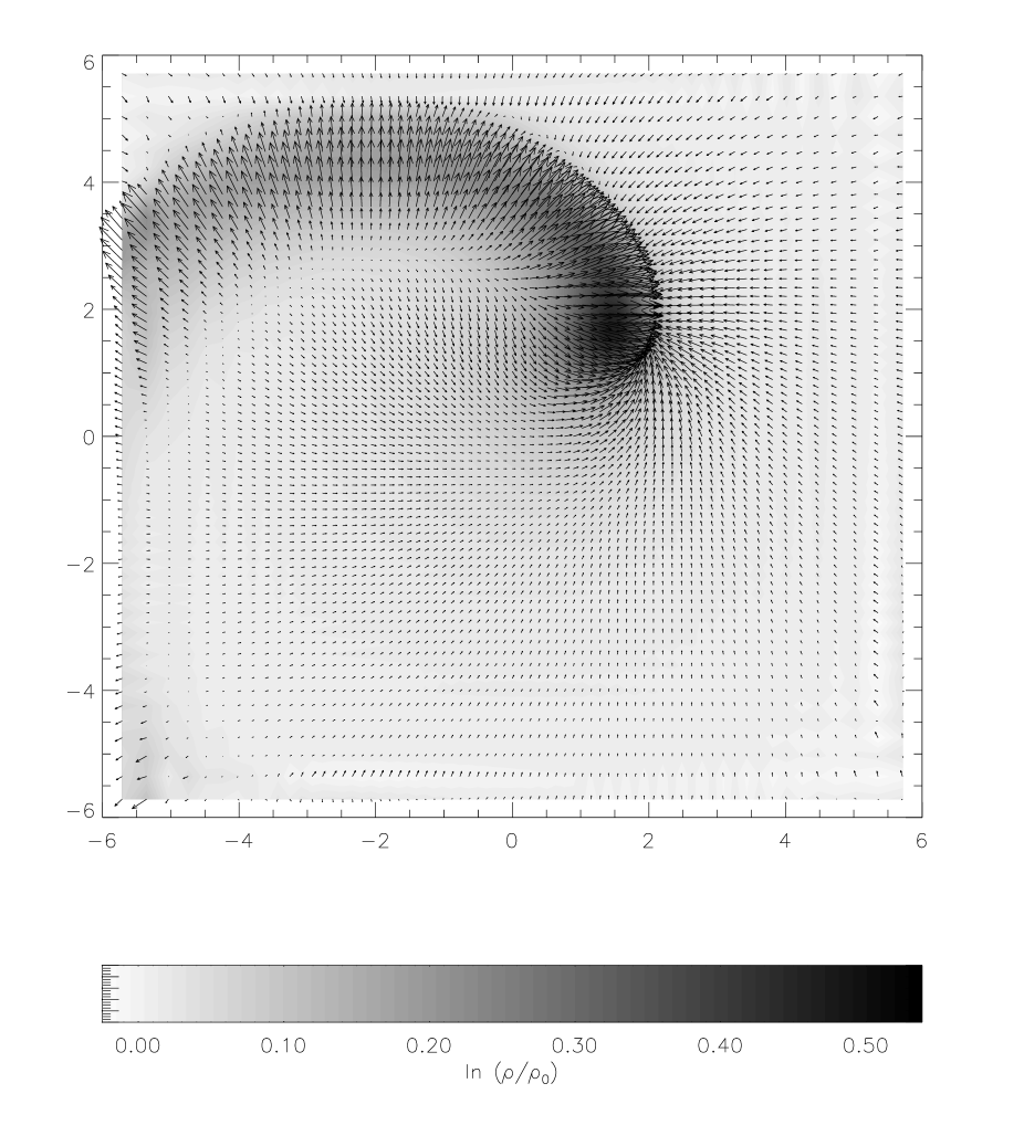
Figure 3: Grey-scale plot of the density enhancement $\ln\left(\rho(\mn@boldsymbol{r},t)/\rho(\mn@boldsymbol{r},0)\right)$, together with velocity vectors, at $z=0$ and $t=26$, for the reference model with $M_{\rm p}=0.3$ and $R_{\rm soft}=0.5$.

Figure 4: Different components and strength of $\mn@boldsymbol{F}_{\rm df}$ versus time for the reference model. $F_{\rm df}$ (solid line), azimuthal component of $\mn@boldsymbol{F}_{\rm df}$ (dotted line) and radial component of $\mn@boldsymbol{F}_{\rm df}$ (dot-dashed line) for a freely decaying perturber. We have taken the absolute values but it is worthwhile to recall that both $\mn@boldsymbol{F}_{\rm df}\cdot\mn@boldsymbol{V}$ and $\mn@boldsymbol{F}_{\rm df}\cdot\hat{\mn@boldsymbol{e}}_{\mn@boldsymbol{r}}$ have negative values. The temporal evolution of $F_{{\rm df},r}$ (triple dot-dashed line) and $F_{{\rm df},\psi}$ (dashed line) for a perturber forced to rotate in a circular orbit with $R_{\rm p}(0)=4$ are also plotted.

The satellite’s angular momentum per unit mass, $J_{\rm p}$, and orbital radius are shown in Fig. 2 as a function of time. We see that the angular momentum decreases almost linearly with time (solid line). A snapshot of the density enhancement and the velocity field at the plane $z=0$ and $t=26$ is shown in Fig. 3. The strength of the radial and azimuthal components of $\mn@boldsymbol{F}_{\rm df}$, in units of $4\pi G^{2}M^{2}_{\rm p}\rho_{0}/c_{\rm s}^{2}$ ($\rho_{0}\equiv\rho(\mn@boldsymbol{r},0)$ hereafter) evaluated at the instantaneous position of the satellite (the ‘dimensionless force’ hereafter), are presented in Fig. 4 for the standard model. As expected, the dimensionless force saturates since the direction of $\mn@boldsymbol{V}$ changes and, consequently, the wake behind the body effectively ‘restarts’. The force shows some oscillations caused by the combination of the interaction of the satellite with its own wake, together with small epicyclic motions of the satellite. For a perturber forced to rotate in its originally circular orbit at constant velocity, the azimuthal force is constant with time (dashed line in Fig. 4), reaching a plateau after half an orbital period. Almost no oscillations in the force are seen in this case.

Let us compare the decay rate with the prediction of formulas (5) and (6). Denoting the azimuthal component of the force by $F_{{\rm df},\psi}$, this expression yields for $R_{\rm p}>0.48$ (i.e. in the supersonic regime):

$$\frac{dJ_{\rm p}}{dt}=-\frac{F_{{\rm df},\psi}R_{\rm p}}{M_{\rm p}}=-\frac{4\pi G^{2}M_{\rm p}\rho_{0}R_{\rm p}}{v_{\rm c}^{2}}I_{\rm adi},$$ (18)

where $v_{\rm c}$ is the circular velocity, and $I_{\rm adi}\equiv\ln\Lambda+\frac{1}{2}\ln\left(1-{\mathcal{M}}^{-2}\right)$ a dimensionless quantity. From $J_{\rm p}=v_{\rm c}R_{\rm p}$ we have

$$\frac{dR_{\rm p}}{dt}=v_{\rm c}^{-1}\left[2-\frac{3}{2}\frac{R_{\rm p}^{2}}{R_{\rm p}^{2}+1}\right]^{-1}\frac{dJ_{\rm p}}{dt}.$$ (19)

It is noted that now $\rho_{0}$ and ${\mathcal{M}}$ depend on the position. In order to integrate Eq. (19), the only remaining unknown is $\ln\Lambda$. Since $\ln\Lambda$ is no longer a linear function of time, we assume that $I_{\rm adi}$ takes the following values for ${\mathcal{M}}>1$

$$I_{\rm adi}=\left\{\begin{array}[]{ll}\ln\left(\frac{v_{\rm c}t}{r_{\rm min}}\right)+\frac{1}{2}\ln{\mathcal{S}}_{\mathcal{M}}&\mbox{${\rm if}\;\;\;\;\tau<t<t_{\rm c}$}\\ {t\over\tau}\left[\ln\left(\frac{{\mathcal{M}}}{{\mathcal{M}}-1}\right)+\frac{1}{2}\ln{\mathcal{S}}_{\mathcal{M}}\right]&\mbox{${\rm if}\;\;\;\;t<\tau<t_{\rm c}$}\\ \ln\left(\frac{v_{\rm c}t_{\rm c}}{r_{\rm min}}\right)+\frac{1}{2}\ln{\mathcal{S}}_{\mathcal{M}}&\mbox{${\rm if}\;\;\;\;\tau<t_{\rm c}<t$}\end{array}\right.$$ (20)

where

$$\tau\equiv{r_{\rm min}\over v_{\rm c}-c_{\rm s}},\quad{\mathcal{S}}_{\mathcal{M}}\equiv 1-{\mathcal{M}}^{-2},\quad t_{\rm c}\equiv{\beta R_{\rm p}\over v_{\rm c}+c_{\rm s}},$$ (21)

with $\beta$ being a free parameter which is chosen to match the values of $J_{\rm p}(t)$ and $R_{\rm p}(t)$ obtained numerically. The minimum radius is taken to be $r_{\rm min}=2.25R_{\rm soft}$, as was inferred for homogeneous media (Paper I) provided that the softening radius is larger or equal to the accretion radius. For $t<\tau<t_{\rm c}$ a linear interpolation has been adopted. For times such that $t_{\rm c}<\tau$, it is difficult to suggest any prescription from the linear theory. We therefore assume that the value remains approximately unchanged compared to the value it has got just before coming into that interval. However, this assumption is not completely satisfactory for bodies moving initially at Mach numbers close to $1$. Therefore we additionally assume that

$$I_{\rm adi}={t\over\tau}\left[\ln\left(\frac{{\mathcal{M}}}{{\mathcal{M}}-1}\right)+\frac{1}{2}\ln{\mathcal{S}}_{\mathcal{M}}\right]$$ (22)

if $t<\tau$ and ${\mathcal{M}}>1$, regardless of the condition $\tau<t_{\rm c}$.

For ${\mathcal{M}}<1$ and a homogeneous background the linear theory is not able to capture the temporal evolution of the drag force but just the asymptotic values; see Eq. (6). As a consequence, for a body moving on a curved orbit, no reliable estimate of the drag force can be proposed straightforward. In the following we shall refer to Eq. (6) together with Eqs (20),(22) as the Local Approximation Prescription (LAP). It is ‘local’ in the sense that the force depends only on quantities at the instantaneous position of the satellite even though, of course, the wake extends far away beyond the satellite. At this stage it becomes clear that the LAP may fail at least for ${\mathcal{M}}$ close to or less than unity.

Figure 5: (a) Temporal evolution of the angular momentum (per unit mass) for the isothermal model with $M_{\rm p}=0.5$, $R_{\rm soft}=0.5$ and $R_{\rm p}(0)=4$ (solid line) and for an identical perturber but initially at $R_{\rm p}(0)=6$ (dashed line). Panel (b) is like panel (a) but now $R_{\rm soft}=1$ and $R_{\rm p}(0)=4$. The predictions by LAP with different $\beta$ are also plotted for the perturbers initially at $R_{\rm p}(0)=4$. LAP overestimates the drag when the distance of perturber to the centre becomes comparable to $R_{\rm soft}$.

The results of the integration for the reference model are plotted as dotted lines in Fig. 2 for $\beta=3.1$. We see that it agrees closely with the numerical values. Part of the success of Eqs (20)-(22) resides in the fact that the condition $\tau<t_{\rm c}$ is satisfied very soon, at $R_{\rm p}\simeq 3.5$, for the present case. However, it may be somewhat different for perturbers moving with Mach numbers close to $1$ for a significant interval of time. This case will be considered in Sect. 4.3.

We ran a model which was identical to the reference model except that the perturber mass was increased to $M_{\rm p}=0.5$. The results of the simulation are plotted in Fig. 5a, together with LAP curves of different $\beta$. There is very good agreement with the LAP for $\beta=3.1$. In general, it is found that a change of a factor three in the mass of the perturber produces a slight variation of about five per cent in the azimuthal component of the dimensionless drag force. Fig. 5a also shows $J_{\rm p}(t)$ for the same perturber but initially at orbital radius $R_{\rm p}=6.0$. Once the angular momentum has decayed to $6.0$ the further evolution is quite similar to the evolution of $J_{\rm p}$ starting at $6.0$.

A new run was done for $M_{\rm p}=0.5$ and $R_{\rm soft}=1$. The evolution of $J_{\rm p}$ is plotted in Fig 5b. Again the LAP using $\beta=3.1$ reproduces reasonably well its evolution.

For simulations with resolutions $120\times 120\times 54$ the change in the drag force is less than 0.5 per cent.

A measure of the robustness of the fitting formulae is given by the dispersion of $\beta$ for forced circular orbits of different radii, which will be referred to as $\beta_{\rm cir}$. Using for $\beta_{\rm cir}$ the expression

$$\beta_{\rm cir}=\frac{r_{\rm min}}{R_{\rm p}}\frac{1+{\mathcal{M}}^{-1}}{(1-{\mathcal{M}}^{-2})^{1/2}}\exp\left(I_{\rm adi}\right),$$ (23)

with $I_{\rm adi}$ being the asymptotic value of the azimuthal component of the force obtained numerically, we have $\beta_{\rm cir}=2.6,2.9,3.2$ and $3.5$ for circular orbits of radii $R_{\rm p}=4,3,2$ and $1.5$, respectively. The rotation velocities were taken according to the rotation curve of the Plummer model. If the perturber moves on a circular orbit of radius $R_{\rm p}=4$ but ${\mathcal{M}}=1.61$, $\beta_{\rm cir}$ is found to be $3.6$ (see Table 1). These results suggest that $\beta_{\rm cir}$ depends on ${\mathcal{M}}$, but could also contain information about the global density profile. In the inner regions $\beta_{\rm cir}$ should also contain the effect of the excitation of gravity waves. Strong resonances occur when the local Brunt-Väisälä frequency matches the orbital frequency of the perturber. The existence of resonances depends strongly on the temperature profile in the inner regions and require in general a large-scale entropy gradient in that region (Balbus & Soker 1990; Lufkin et al. 1993). For satellite galaxies the amplification of gravity waves, if any, may only take place in the very inner part of the parent galaxy. However, other effects, such as mass stripping and tidal deformation of the satellite galaxy as well as friction with the luminous and collisionless parts of the galaxy, may play an important role as far as dynamical evolution of the satellite galaxy is concerned.

For fixed rotation curve, the parameter $\beta$ may have some dependence on other variables of the system such as $\Gamma$. This question will be considered in the next few sections.

4.2 Testing the accuracy. Constant-velocity perturbers in a homogeneous background

A measure of the accuracy of our 3D simulations is given by comparing the force of dynamical friction experienced by a perturber moving on a straight-line orbit with constant velocity $\mn@boldsymbol{V}$ in a uniform and isothermal medium, with the axisymmetric simulations described in Paper I, which had higher resolution. In Fig. 6 we plot the drag force experienced by a body that moves in the $x$-direction using the same resolution as that in our reference model, together with the values obtained in high-resolution simulations. The initial position of the body is $(-4,-4,0)$ and it travels at constant velocity with Mach number $0.75$ (bottom lines) and $1.12$ (upper lines). In the supersonic experiments the ratio between $R_{\rm soft}$ and the accretion radius defined as $2GM_{\rm p}/V^{2}$, was $1.5$, with a softening radius of $0.5$. As long as the body is within the region $|x|<6$ the accuracy of the force is better than five per cent.

Figure 6: Dimensionless drag force experienced by a body moving according to $\mn@boldsymbol{R}_{\rm p}=(-4+Vt,-4,0)$ in a unperturbed background of constant density. The solid line shows the numerical results for high resolution axisymmetric simulations whereas the dotted line is for 3D simulations with resolution as in the reference model.

Figure 7: Rotation curve for the Plummer model (solid line), and the sound speed profiles for $\Gamma=5/3$ (dot-dashed line), $\Gamma=1.4$ (triple dot-dashed line), and $\Gamma=1.2$ (dashed line).

4.3 Polytropic gas

Let us now consider the same perturber with $R_{\rm soft}=0.5$ and mass $M_{\rm p}$ that is forced to move on a circular orbit in a polytropic gas and compute the value of $\beta_{\rm cir}$ that matches the results. We do this for models which have different polytropic indices $\Gamma$. The rotation curve is assumed to be the same as in the reference model. Rotation curve and sound speed profiles for models with different pairs $(\Gamma,c_{\rm s0})$ are drawn in Fig. 7. Since they have different polytropic indices we will specify each of these models by just giving their polytropic index. For the model with polytropic index $5/3$, the Mach number of the perturber at $R_{\rm p}=4$ is approximately the same as in the reference model. The corresponding values of $\beta_{\rm cir}$ for each value of $\Gamma$ are given in Table 1, except for the case $\Gamma=5/3$ at $R_{\rm p}=2$ because for that orbit $t_{\rm c}\ll\tau$. Table 1 suggests a remarkable dependence of $\beta_{\rm cir}$ on ${\mathcal{M}}$, as well as on $\Gamma$. This reflects the fact that the asymptotic value of the azimuthal component of the dimensionless force is not sensitive to the Mach number whenever ${\mathcal{M}}=1.1$–$1.6$. Given $\Gamma$ and $R_{\rm p}$, the variation of the force in that interval of ${\mathcal{M}}$ is less than five per cent.

Table 1: $\beta_{\rm cir}$ as defined in Eq. (23) for models which have different $\Gamma$. The body has a mass of $0.3$, softening radius $0.5$, and is forced to move in a circular orbit of radius $R_{\rm p}$ with a Mach number which may not correspond to the rotation curve of the Plummer model. If $\beta_{\rm cir}$ are displayed in the same row for both $R_{\rm p}=4$ and $R_{\rm p}=2$, it means that they correspond to the rotation curve given by the model.

$\Gamma$	${\mathcal{M}}$	$\beta_{\rm cir}$	${\mathcal{M}}$	$\beta_{\rm cir}$
	$R_{\rm p}=4$	$R_{\rm p}=4$	$R_{\rm p}=2$	$R_{\rm p}=2$
1.0	1.16	2.6	1.45	3.2
1.0	1.61	3.6
1.2	1.61	2.8	1.67	3.1
1.2	1.27	2.1
1.2			1.41	2.7
1.4	1.27	2.2	1.41	2.7
1.4	1.61	3.0
1.4			1.67	3.0
5/3	1.12	2.4	1.09	…

For sinking orbits the value of $\beta$ may differ somewhat from the median of $\beta_{\rm cir}$ because the orbit of the body loses correlation with its wake faster than in a fixed circular orbit. The case of $\Gamma=5/3$ is particularly interesting because then $t_{\rm c}<\tau$ for a remarkably broad range of $R_{\rm p}$. The $\beta$-parameter seems to be rather arbitrary in that range. In Fig. 8 the evolution of $J_{\rm p}$ and $R_{\rm p}$ is plotted for $M_{\rm p}=0.3$ (upper panel) and $M_{\rm p}=0.1$ (bottom panel). In both simulations $\Gamma=5/3$. The prediction of the LAP is plotted as dotted lines for $\beta=2.1$ in both cases. In the first case the decay is so fast that the LAP might no longer be a good approximation (upper panel). However, even for slower decays (the case of $M_{\rm p}=0.1$) the LAP is not able to give reliable values of the force in the subsonic regime. In fact, Eq. (6) overestimates significantly the friction, mainly because of two reasons; firstly, the wake must restart as a consequence of the curvature of the orbit and, secondly, the orbital radius and size of the object become comparable.

Figure 8: In the left panels it is shown the evolution of the angular momentum (per unit mass) for the model with $\Gamma=5/3$ and $M_{\rm p}=0.3$ (solid line of upper panel) and $M_{\rm p}=0.1$ (bottom panel). The corresponding evolution of the radial distance of the perturber is plotted as solid lines in the right panels. Dotted lines show the predictions of the LAP using $\beta=2.1$. LAP fails as soon as the motion becomes slightly supersonic.

Figure 9: Solid lines show the value of the radial component of the force $\mn@boldsymbol{F}_{\rm df}$ for the $\Gamma=1$ model with $M_{\rm p}=0.3$ (at the top) and for $\Gamma=5/3$ and $M_{\rm p}=0.1$ (at the bottom). The azimuthal components are plotted with dashed-lines, whilst the radial ones in dotted lines.

Since for the model with $\Gamma=5/3$ the typical velocities $v_{\rm c}/c_{\rm s}$ lie in the range $1.0$–$1.2$ at the radius interval $\in[2,4]$, one would expect, according to Eq. (5), a larger value of the dimensionless drag force in this case compared to the isothermal gas model in which the body moves with higher values of ${\mathcal{M}}$. A comparison between those forces for $\Gamma=5/3$ and $\Gamma=1$ is given in Fig. 9. Unexpectedly, the dimensionless drag force is stronger in the run corresponding to $\Gamma=1$.

Finally, the evolution of $J_{\rm p}$ of a perturber of mass $0.3$ is drawn in Fig. 10 for $\Gamma=1.4$ as well as for $\Gamma=1.2$. The $\beta$-parameter was $2.2$ and $3.1$, respectively. Clearly, the LAP becomes inaccurate as soon as the body becomes transonic.

Figure 10: Decay of $J_{\rm p}$ of a perturber of mass $M_{\rm p}=0.3$ initially in circular orbit, for different values of $\Gamma$. The dotted lines indicate the prediction of the LAP.

4.4 Non-circular orbits in the Plummer model

The dependence of the orbital sinking times on the eccentricity of the orbit is of interest for the statistical analysis of merging rates of substructure in the cosmological scenario (e.g. Lacey & Cole 1993; Colpi et al. 1999), and for the theoretical eccentricity distributions of globular clusters and galactic satellites [van den Bosch et al. 1999]. On the one hand, the hierarchical clustering model predicts that most of the satellite’s orbits have eccentricities between $0.6$ and $0.8$ (Ghigna et al. 1998). On the other hand, the median value of the eccentricity of an isotropic distribution is typically $0.6$ [van den Bosch et al. 1999]. Here we explore the dependence on eccentricity for dynamical friction in a gaseous sphere in the Plummer potential. The non-singular isothermal sphere is considered in the next subsection.

Figure 11: Panel (a) shows the orbital angular momentum in units of the initial value for orbits having initially the same energy but different eccentricities in the Plummer model with $\Gamma=1$. $M_{\rm p}=0.4$ and $R_{\rm soft}=0.5$ were taken. In panels (b), (c) and (d) the corresponding orbits in the plane $(x,y)$ are presented for initial circularities $0.75$, $0.6$ and $0.5$, respectively.

We shall discuss the sinking rate in terms of the angular momentum half-time, $t_{1/2}$, the time after which the perturber has lost half of its initial orbital angular momentum. Fig. 11 shows the dynamical evolution of the satellite on bound orbits having initially equal energies but different eccentricities ($J_{\rm p}$ is in units of the initial value). Here we have used the polytropic model with $\Gamma=1$. A good fit to the numerical results is $t_{1/2}\propto\epsilon^{-0.4}$, where $\epsilon$ is the initial circularity, $\epsilon\equiv J_{\rm p}(E)/J_{\rm p;cir}(E)$, the ratio between the orbital angular momentum and that of the circular orbit having the same energy $E$. The dynamical friction time scale is found to increase with increasing eccentricity. This finding makes a clear distinction between dynamical friction in stellar and gaseous systems. In fact, the dynamical friction time scale has been obtained by direct N-body simulations and in the linear response theory suggesting $t_{1/2}\propto\epsilon^{0.4}$ for bodies embedded in a truncated non-singular isothermal sphere of collisionless matter (van den Bosch et al. 1999; Colpi et al. 1999). A notorious difference between stellar and gaseous backgrounds is that the gaseous force is strongly suppressed when the perturber falls in the subsonic regime along its non-circular orbit. In order to discern how much the above result depends on the model, we will consider in the next subsection the angular momentum half-time for bodies orbiting in the non-singular isothermal sphere.

4.5 Sinking perturbers in the non-singular isothermal sphere

The flat behaviour of the rotation curves of spiral galaxies strongly suggests the existence of isothermal dark halos around them. That is the reason why most of the studies about dynamical friction assume an isothermal sphere as the standard background. In the case of a self-gravitating sphere of gas, the non-singular isothermal sphere is also a natural choice. For instance, we may consider the dynamical friction of condensed objects in early stages of a star cluster or a galaxy, in which most of the mass of the system is gas. The gas component is expected to follow the non-singular isothermal sphere out to great radii.

We use the King approximation to the inner portions of an isothermal sphere, with softening radius $R_{\rm G}$ and central density $\rho_{\rm G}(\mn@boldsymbol{0})$, i.e.

$$\phi_{\rm G}=-4\pi G\rho_{\rm G}(\mn@boldsymbol{0})R_{\rm G}^{2}\frac{1}{x}\ln\left(x+\sqrt{1+x^{2}}\right),$$ (24)

with $x=r/R_{\rm G}$ [Binney & Tremaine 1987]. Our units are still $G=R_{\rm G}=\rho(\mn@boldsymbol{0},0)=1$. Even though the rotation curve adopted is very similar to that of the Plummer model, the detailed evolution, such as the dependence of the decay rate on eccentricity or the level of circularization of the orbits, may be somewhat different. For the sake of brevity, we only present the results for the case where the Euler and continuity equations were solved together with the entropy equation.

Figure 12: The orbital angular momentum in units of the initial value for orbits having initially the same energy but different circularities in the King model.

Fig. 12 shows the decay of a perturber with $M_{\rm p}=0.3$ and $R_{\rm soft}=0.5$ in a King model with $\rho_{\rm G}=1$, i.e. pure gaseous sphere, for different circularities. There are no appreciable variations of the decay time for different initial circularities. In order to gain deeper insight into the differences between the dynamical friction timescale in an isothermal sphere of gas instead of collisionless matter, we have computed the circularity at the times when the orbital phase is zero (Fig. 13). The circularity does not change at all for initially circular orbits. For eccentric orbits, deviations in the circularity occur but there is no net generation. The lack of dependence of the decay times on circularity, together with the absence of any significant amount of circularization, lead us to conclude that dynamical friction in a gaseous isothermal sphere is not able to produce changes in the distribution of orbital eccentricities. Mass stripping which could lead to circularization has been ignored.

Figure 13: Circularity as a function of time for the same situation as in Fig. 12. The circularities are computed at the time when the orbital phase is zero.

5 Discussion and conclusions

In this paper we have presented simulations of the decay of a rigid perturber in a gaseous sphere. As a first approximation, both the mass stripping and the barycentric motion of the primary were neglected. In addition, the softening radii of the perturbers were taken a few times larger than the accretion radius. Simulations of the evolution of very compact bodies ($R_{\rm soft}\ll R_{\rm ac}$), such as black holes in a spherical background are numerically very expensive.

The Linear Approximation Prescription is able to explain successfully the evolution of the perturber provided the (i) decay is not too fast, (ii) the motion is supersonic and (iii) the body is not too close to the center to avoid that $R_{\rm p}$ becomes comparable to $R_{\rm soft}$. In our simulations, the angular momentum of the perturber decays almost linearly with time. Generally speaking, the associated Coulomb logarithm should depend on the distance of the perturber to the centre and on its Mach number. However, the evolution of a free perturber is relatively well described by just a linear dependence of the maximum impact parameter of the Coulomb logarithm on radius, except very close to the centre where the time averaged Mach number is less than unity.

In Chandrasekhar’s formalism the Coulomb logarithm is often approximated by the logarithm of the ratio of the maximum to minimum impact parameters of the perturber. In a singular isothermal sphere of collisionless matter, the time for an approximately circular orbit to reach the center is

$$\tau_{\rm s}=1.2\frac{r_{\rm cir}^{2}V_{\rm cir}}{GM_{\rm p}\ln\frac{b_{\rm max}}{b_{\rm min}}},$$ (25)

where $b_{\rm max}$ is roughly the virial radius of the primary and $b_{\rm min}$ is of the order of the softening radius of the perturber [Binney & Tremaine 1987]. We have confirmed numerically Ostriker’s suggestion that the Coulomb logarithm should be replaced by

$$\ln\frac{b_{\rm max}}{b_{\rm min}}\rightarrow\frac{1}{0.428}\ln\left(\eta\frac{R_{\rm p}(t)}{R_{\rm soft}}\right)$$ (26)

for the gaseous case, with $\eta\simeq 0.35$, and independent of the eccentricity. For very light perturbers in near-circular orbits (objects with mass fractions smaller than one per cent), the time scale for dynamical friction is a factor $2$ smaller in the case of a gaseous sphere than in corresponding stellar systems (e.g. globular clusters in the Galactic halo). This factor is somewhat smaller when $R_{\rm p}$ becomes comparable to a few $R_{\rm soft}$. The weak dependence of the decay times on eccentricity suggests that more eccentric orbits of merging satellites should not decay more rapidly in the halo during the epoch in which matter is mainly gas. Thus, they do not touch the disc at an earlier time than less eccentric orbits. Our simulations give support to the idea that dynamical friction does not produce changes in the distribution of orbital eccentricities.

The analysis must be modified if one wishes to account for the existence of clouds in a non-uniform medium. So far, in a variety of systems it is assumed that the perturber has condensed from fragmentation of the gas; thus, the gaseous component must be thought of as being distributed in clumps or clouds even more massive than the ‘perturbers’. In certain situations, compact perturbers may not be dragged but heated (e.g. Gorti & Bhall 1996). For this reason one may be pessimistic towards a recent suggestion by Ostriker (1999) that, because of the contribution of the gaseous dynamical friction force, young stellar clusters should appear significantly more relaxed than usually expected.

Appendix A Description of the code

We solve Eqs (7)–(12) on a nonuniform cartesian mesh, $(x,y,z)$. This is accomplished using a coordinate transformation to a uniform mesh, $(\xi,\eta,\zeta)$, with

$$x=x(\xi)={\xi\over 1-(\xi/L_{\xi})^{4}},$$ (27)

where $L_{\xi}$ is a length parameter, and similarly for $y=y(\eta)$ and $z=z(\zeta)$. The transformed equations are solved using sixth order centred finite differences,

$$\left({\partial^{n}f\over\partial\xi^{n}}\right)_{i}={1\over\Delta\xi^{n}}\sum_{j=-3}^{3}c_{j}^{(n)}f(x_{i+j})$$ (28)

for the $n$th $\xi$-derivative. The coefficients $c_{j}^{(n)}$ are given in Table 2. The expressions for the $\eta$ and $\zeta$ derivatives are analogous to Eq. 28.

Table 2: Coefficients for the derivative formulae

$j$	0	$\pm 1$	$\pm 2$	$\pm 3$
$c_{j}^{(1)}\times 60$	0	$\pm 45$	$\mp 9$	$\pm 1$
$c_{j}^{(2)}\times 180$	$-490$	$+270$	$-27$	$+2$

The corresponding $x$-derivative of a function $f(\xi(x))$ is obtained using the chain rule, so

$${\partial f\over\partial x}={\partial\xi\over\partial x}{\partial f\over\partial\xi}={u^{\prime}\over x^{\prime}},$$ (29)

where primes denote $\xi$-derivatives. For the second derivative we have

$${\partial^{2}f\over\partial x^{2}}={u^{\prime\prime}x^{\prime}-u^{\prime}x^{\prime\prime}\over x^{\prime 3}}.$$ (30)

Again, the expressions for the $y$ and $z$ derivatives are analogous. Since the scheme is accurate to $\Delta\xi^{6}$, $x$-derivatives are accurate to $\Delta x^{6}(\xi)$, which varies of course across the mesh.

The third order Runge-Kutta scheme can be written in three steps (Rogallo 1981):

$$\begin{array}[]{lll}\mbox{1st step:}&\quad f=f+\gamma_{1}\Delta t\dot{f},&\quad g=f+\zeta_{1}\Delta t\dot{f},\\ \mbox{2nd step:}&\quad f=g+\gamma_{2}\Delta t\dot{f},&\quad g=f+\zeta_{2}\Delta t\dot{f},\\ \mbox{3rd step:}&\quad f=g+\gamma_{3}\Delta t\dot{f},&\end{array}$$ (31)

where

$$\gamma_{1}={8\over 15},\quad\gamma_{2}={5\over 12},\quad\gamma_{3}={3\over 4},\quad\zeta_{1}=-{17\over 60},\quad\zeta_{2}=-{5\over 12}.$$ (32)

Here, $f$ and $g$ always refer to the current value (so the same space in memory can be used), but $\dot{f}$ is evaluated only once at the beginning of each of the three steps. The length of the time step must always be a certain fraction of the Courant-Friedrich-Levy condition, i.e. $\Delta t=k_{\rm CFL}\Delta x/U_{\max}$, where $k_{\rm CFL}\leq 1$ and $U_{\max}$ is the maximum transport speed in the system.

The nonuniform mesh allows us to move the boundaries far away, so the precise location of the boundaries should not matter. In all cases we have used open boundary conditions by calculating derivatives on the boundaries using a one-sided difference formula accurate to second order. This condition proved very robust and satisfied our demands.

Equations (7)–(12) are solved in non-conservative form. This is sufficiently accurate because of the use of high order finite differences and because the solutions presented in this paper are sufficiently well resolved.

References

- [Balbus & Soker 1990] Balbus, S. A., Soker, N. 1990, ApJ, 357, 353
- [Balsara, Livio & O’Dea 1994] Balsara, D., Livio, M., O’Dea, C. P. 1994, ApJ, 437, 83
- [Bekenstein & Maoz 1992] Bekenstein, J., Maoz, E. 1992, ApJ, 390, 79
- [Binney & Tremaine 1987] Binney, J., Tremaine, S. 1987, Galactic Dynamics (Princeton: Princeton Univ. Press)
- [Chandrasekhar 1943] Chandrasekhar, S. 1943, ApJ, 97, 255
- [Chandrasekhar & von Neumann 1942] Chandrasekhar, S., von Neumann, J. 1942, ApJ, 95, 489
- [Colpi 1998] Colpi, M. 1998, ApJ, 502, 167
- [Colpi et al. 1999] Colpi, M., Mayer, L., Governato, F. 1999, ApJ, 525, 720
- [Cora et al. 1997] Cora, S. A., Muzzio, J. C., Vergne, M. M. 1997, MNRAS, 289, 253
- [De Paolis et al. 1995] De Paolis, F., Ingrosso, G., Jetzer, P. et al. 1995, A&A, 299, 647
- [De Paolis et al. 1999] De Paolis, F., Ingrosso, G., Jetzer, P., Roncadelli, M. 1999, ApJ, 510, L103
- [Gerhard & Silk 1996] Gerhard, O., Silk, J. 1996, ApJ, 472, 34
- [Ghigna et al. 1998] Ghigna, S., Moore, B., Governato, F., Lake, G., Quinn, T., Stadel, J. 1998, MNRAS, 300, 146
- [Gorti & Bhatt 1996] Gorti, U., Bhatt, H. C. 1996, MNRAS, 278, 611
- [Isihara 1971] Isihara, A. 1971, Statistical Physics, Academic Press, New York
- [Kandrup 1983] Kandrup, H. E. 1983, Ap&SS, 97, 435
- [Kley, Shankar & Burkert 1995] Kley, W., Shankar, A., Burkert, A. 1995, A&A, 297, 739
- [Lee 1968] Lee, E. P. 1968, ApJ, 151, 687
- [Lin & Tremaine 1983] Lin, D. N. C., Tremaine, S. 1983, ApJ, 264, 364
- [Lufkin, Balbus & Hawley 1993] Lufkin, E. A., Balbus, S. A., Hawley, J. F. 1995, ApJ, 446, 529
- [Maoz 1993] Maoz, E. 1993, MNRAS, 263, 75
- [Ostriker 1999] Ostriker, E. C. 1999, ApJ, 513, 252
- [Ostriker & Davidsen 1968] Ostriker, J. P., Davidsen, A. F. 1968, ApJ, 151, 679
- [Pfenniger, Combes & Martinet 1994] Pfenniger, D., Combes, F., Martinet, L. 1994, A&A, 285, 79
- [Prugniel & Combes 1992] Prugniel, Ph., Combes, F. 1992, A&A, 259, 25
- [Rephaeli & Salpeter 1980] Rephaeli, Y., Salpeter, E. E. 1980, ApJ, 240, 20
- [Rogallo1981] Rogallo, R. S. 1981, Numerical experiments in homogeneous turbulence, NASA Tech. Memo. 81315
- [Ruderman & Spiegel 1971] Ruderman, M. A., Spiegel, E. A. 1971, ApJ, 165, 1
- [Ruffert 1996] Ruffert, M. 1996, A&A, 311, 817
- [Sánchez-Salcedo & Brandenburg 1999] Sánchez-Salcedo, F. J., Brandenburg, A. 1999, ApJ, 522, L35 (Paper I)
- [Sciama 2000] Sciama, D. W. 2000, MNRAS, 312, 33
- [Shankar, Kley & Burkert 1993] Shankar, A., Kley, W., Burkert, A. 1993, A&A, 274, 995
- [Shima, Matsuda, Takeda & Sawada 1985] Shima, E., Matsuda, T., Takeda, H., Sawada, K. 1985, MNRAS, 217, 367
- [Shima, Matsuda & Inaguchi 1986] Shima, E., Matsuda, T., Inaguchi, T. 1986, MNRAS, 221, 687
- [Tittley et al. 1999] Tittley, E. R., Couchman, H. M. P., Pearce, F. R. 1999, MNRAS (submitted), astro-ph/9911017
- [Sandquist et al. 1998] Sandquist, E. L., Taam, R. E., Chen, X., Bodenheimer, P., Burkert, A. 1998, ApJ, 500, 909
- [Spergel & Steinhardt 2000] Spergel, D. N., Steinhardt, P. J. 2000, Phys. Rev. Lett., 84, 3760
- [Taam et al. 1994] Taam, R. E., Bodenheimer, P., Rózyczka, M. 1994, ApJ, 431, 247
- [van den Bosch et al. 1999] van den Bosch, F. C., Lewis, G. F., Lake, G., Stadel, J. 1999, ApJ, 515, 50
- [Walker 1999] Walker, M. 1999, MNRAS, 308, 551
- [Walker & Wardle 1998] Walker, M., Wardle, M. 1998, ApJ, 498, L125
- [Zamir 1992] Zamir, R. 1992, ApJ, 392, 65