The bright 175 $\mu$m knots of the Andromeda Galaxy

Abstract

Discrete far-infrared (FIR) sources of M 31 are identified in the ISO 175 $\mu$m map and characterized via their FIR colours, luminosities and masses in order to reveal the nature of these knots. With our spatial resolution of 300 pc at M 31’s distance, the FIR knots are clearly seen as extended objects with a mean size of about 800 pc. Since this appears too large for a single dust cloud, the knots might represent several clouds in chance projection or giant cloud complexes.

The 175 $\mu$m data point provides crucial information in addition to the IRAS 60 and 100 $\mu$m data: At least two $\lambda$^-2 modified Planckian curves with temperatures of about 40 K and 15-21 K are necessary to fit the spectral energy distributions (SEDs) of the knots. Though they show a continuous range of temperatures, we distinguish between three types of knots – cold, medium, warm – in order to recognize trends. Comparisons with radio and optical tracers show that – statistically – the cold knots can be identified well with CO and H I radio sources and thus might represent mainly molecular cloud complexes. The warm knots coincide with known H II regions and supernova remnants. The medium knots might contain a balanced mixture of molecular clouds and H II regions. The cold knots have a considerable luminosity and their discovery raises the question of hidden star formation.

Though the optically dark dust lanes in M 31 generally match the FIR ring, surprisingly we do not find a convincing coincidence of our knots with individual dark clouds, which might therefore show mainly foreground dust features.

The ratio of FIR luminosity to dust mass, $L/M$, is used to measure the energy content of the dust. It can originate from both the interstellar radiation field and still embedded stars recently formed. The knots have a clear $L/M$ excess over the rest of M31, providing evidence that they are powered by star formation in addition to the interstellar radiation field. Furthermore, the $L/M$ ratio of the warm knots is comparable to that of Galactic H II regions like M 42 or NGC 2024, while that of the cold knots still reaches values like in the average Orion complex. Thus both the warm and even the cold knots are interpreted as containing large cloud complexes with considerable ongoing star formation.

1 Introduction

The ISO map of M 31 at 175 $\mu$m is dominated by a concentric ring structure containing numerous individual knots (Haas et al. Haas98 (1998)). A similar structure was found in the IRAS maps (Habing et al. Hab84 (1984), Walterbos & Schwering (1987), Xu & Helou Xu96 (1996)), in radio continuum surveys (Berkhuijsen et al. Ber83 (1983), Beck et al. Beck+98 (1998)), in the distribution of OB associations (van den Bergh Ber91 (1991)), H II regions (Baade & Arp Baa64 (1964), Pellet et al. (1978)), and H I gas (Sofue et al. (1981), Cram et al. (1980), Brinks & Shane Bri84 (1984)), and in several other observations (see Hodge (1990)). It seems that the star formation in M 31 is concentrated on these rings and is very low in the inter-ring regions (e.g. Devereux et al. (1994), Xu & Helou Xu96 (1996)). Most recently, this has also been suggested from mid-infrared spectra observed with ISOCAM (Cesarsky et al. (1998)), as well as from more detailed CO (Loinard et al. (1996), Loinard & Allen (1998), Loi+99 (1999), Neininger et al. Nei+98 (1998)) and IR (Pagani et al. Pag+99 (1999)) observations of some inner regions of M 31, mainly concentrated on the SW half of the galaxy. Based on the 175 $\mu$m map the cold dust content has been revealed for the total galaxy (Haas et al. Haas98 (1998)). It turned out to be much colder and about ten times higher than previously detected. Thus the question arises whether we see new, optically highly extinguished regions. Especially the ring exhibits numerous knots bright in the FIR. Their luminosity requires an explanation either via the interstellar radiation field (ISRF) or via deeply embedded young stars possibly hidden to observations at shorter wavelengths.

Therefore, in this paper we concentrate on these discrete FIR sources. We catalogue the 175 $\mu$m knots, compare them with 60 and 100 $\mu$m IRAS data, derive their properties, such as colour, luminosity and mass, and look for coincidence with radio and optical tracers. Finally, the question of star formation in the knots is addressed via the $L/M$ ratio, i.e. the normalized energy content, and compared to that of the total galaxy as well as the Milky Way and regions therein.

Figure 1: Top: $175\mu m$ map displaying the ring structure with the individual knots. Bottom: Finding map displaying the positions of the 47 identified knots.

a) The region around the knots 12, 14, and 15.

b) The region around the knots 34, 38, and 41.

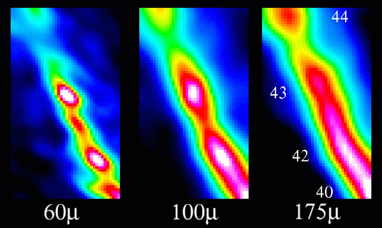
c) The region around the knots 40, 42, 43, and 44.

Figure 2: Detailed maps of the areas around some of the knots at different wavelengths. The 60 and 100 $\mu$m maps are from the IRAS HIRES archive, the 175 $\mu$m map s from Haas et al. (Haas98 (1998)).

2 Identification and flux determination

The 175 $\mu$m map was obtained in February 1997 with ISO’s (Kessler et al. (1996)) photometer ISOPHOT (Lemke et al. (1996)) covering a field of $3^{\circ}\times 1^{\circ}$ oriented along the major axis at PA $39^{\circ}$ with a spatial resolution of about $1.^{\prime}5$. The data reduction and calibration is described in Haas et al. (Haas98 (1998)).

The discrete sources of the 175 $\mu$m map have first been identified visually, then two-dimensional elliptical Gaussians have been fitted over areas of $8^{\prime}\times 8^{\prime}$. In total, 47 sources have been detected above a threshold of 4 sigma of the local background; they are listed in Table 1. Columns (2) and (3) give the 175 $\mu$m position of the sources with an accuracy of about $15^{\prime\prime}$. Column (4) gives an approximation of the knot’s size derived from the average of the FWHMs along the two axes. The sources are catalogued in right ascension order. Fig. 1 shows the distribution of the knots in a map of M 31, and gives a corresponding finding map with the positions for all knots indicated.

Table 1: The catalogued 175 $\mu m$ knots with their reference numbers in column (1). The positions are given in column (2) and (3), an approximated diameter in column (4). The flux densities at 175 $\mu m$ have been derived from the ISO map, the corresponding ones at 60 $\mu m$ and 100 $\mu m$ from the high resolution IRAS maps. Column (8) indicates the classification by spectral appearance. The temperature of the cold component, the mass ratio, the total mass, the luminosity ratio and the total FIR luminosity have been derived by fitting modified Planck functions to the spectra. Column (14) gives the number of the corresponding entry in the 60 $\mu$m point source catalogue of Xu & Helou (Xu96 (1996)) (with uncertain identifications set in brackets), while column (15) lists the detections at other wavelengths (see references below).

(1)	(2)	(3)	(4)	(5)	(6)	(7)	(8)	(9)	(10)	(11)	(12)	(13)	(14)	(15)
No	RA2000	Dec2000	$d$	$\displaystyle\rm\frac{F_{175}}{Jy}$	$\displaystyle\rm\frac{F_{60}}{Jy}$	$\displaystyle\rm\frac{F_{100}}{Jy}$	Type	$\displaystyle\rm\frac{T_{c}}{K}$	$\rm m_{c}/m_{w}$	$\displaystyle\frac{\rm m_{total}}{10^{3}m_{\odot}}$	$\rm L_{c}/L_{w}$	$\displaystyle\frac{\rm L_{total}}{10^{6}L_{\odot}}$	PS60	*)
1	0 39 13.8	40 36 44	$3.^{\prime}6$	4.91	1.59	4.03	II	18.5	152.0	2.702	1.49	2.6	6					E	F
2	0 39 22.4	40 22 15	$6.^{\prime}0$	4.83	1.11	3.45	II	18.2	227.8	2.909	2.02	2.2	3					E	F
3	0 39 41.7	40 29 17	$3.^{\prime}6$	3.64	0.41	2.30	II	18.0	596.5	2.406	4.95	1.4	4						F
4	0 39 43.4	40 21 02	$3.^{\prime}2$	11.68	3.31	11.49	III	21.0	157.1	3.910	3.29	6.2	1			C		E	F	G
5	0 39 51.3	40 53 03	$4.^{\prime}3$	3.73	0.50	2.21	II	18.0	500.0	2.477	4.15	1.5							F
6	0 40 31.4	40 41 06	$4.^{\prime}2$	18.68	0.88	8.40	I	17.0	2300.0	16.253	13.55	6.0	(7)				D		F	G	H
7	0 40 37.6	40 52 51	$3.^{\prime}6$	8.95	0.97	5.57	II	18.0	653.8	6.013	5.43	3.4					D		F	G
8	0 40 39.4	40 36 21	$4.^{\prime}1$	28.82	4.16	15.64	II	17.0	538.5	24.768	3.17	11.1	5						F	G	H
9	0 40 43.1	40 45 51	$3.^{\prime}7$	12.63	0.00	0.16	I										D		F	G
10	0 40 44.2	40 55 51	$3.^{\prime}3$	19.20	1.61	9.88	II	17.0	1043.5	16.969	6.15	6.7				C	D		F	G	H
11	0 40 57.8	40 37 52	$4.^{\prime}5$	23.60	3.28	14.48	II	18.0	488.9	15.571	4.06	9.3					D	E	F	G	H
12	0 40 59.9	41 04 07	$3.^{\prime}0$	27.12	5.64	17.17	II	17.6	287.2	19.138	2.08	11.9	12				D	E	F	G
13	0 41 18.7	40 49 53	$3.^{\prime}0$	25.83	4.57	19.12	II	19.0	316.7	13.463	3.64	11.4					D		F		H
14	0 41 23.6	41 12 23	$3.^{\prime}6$	18.30	3.60	13.40	II	18.5	283.0	10.633	2.77	8.2	18	A			D	E	F	G
15	0 41 34.3	41 08 08	$4.^{\prime}7$	9.14	0.44	4.27	I	17.0	2291.7	7.773	13.50	2.9				C	D				H
16	0 41 44.8	41 17 54	$4.^{\prime}9$	10.22	2.12	6.96	II	18.0	290.9	6.804	2.42	4.6	20	A				E	F
17	0 41 50.4	40 54 09	$6.^{\prime}1$	10.71	0.71	4.32	I	16.3	1454.5	11.309	6.66	3.5					D		F		H
18	0 42 03.4	41 23 24	$4.^{\prime}0$	11.55	0.72	5.23	I	17.0	1555.6	9.895	9.16	3.8		A			D				H
19	0 42 10.2	40 52 09	$4.^{\prime}9$	10.57	1.86	6.86	II	18.0	357.1	7.083	2.97	4.6	10				D		F		H
20	0 42 18.1	41 06 24	$3.^{\prime}5$	8.20	0.91	6.20	III	19.5	733.3	3.890	9.84	3.3	15				D	E
21	0 42 22.1	41 28 09	$3.^{\prime}5$	23.17	4.42	15.41	II	18.0	295.8	14.883	2.46	10.1	25	A	B		D	E	F	G	H
22	0 42 20.8	40 59 09	$5.^{\prime}0$	11.91	0.50	5.97	II	17.5	3250.0	9.185	22.79	3.9					D		F		H
23	0 42 30.1	41 20 09	$4.^{\prime}5$	31.45	7.36	18.48	I	16.5	338.5	31.171	1.67	14.2					D
24	0 42 31.4	40 58 39	$5.^{\prime}0$	14.81	1.18	5.50	I	15.5	1611.1	20.497	5.45	4.8					D		F	G	H
25	0 42 40.7	41 00 39	$4.^{\prime}4$	12.40	1.12	5.48	I	16.3	1117.6	13.453	5.12	4.3					D	E	F	G	H
26	0 42 43.4	41 33 24	$4.^{\prime}5$	27.47	5.56	20.93	II	19.0	270.3	14.179	3.10	12.5	26				D	E	F	G	H
27	0 42 52.7	41 16 09	$4.^{\prime}2$	17.42	19.34	30.62	III	25.0	14.4	2.719	0.85	19.1			B	C	D
28	0 43 00.8	41 37 09	$3.^{\prime}5$	27.12	9.74	26.36	III	20.0	110.7	11.047	1.73	15.7					D		F	G
29	0 43 09.9	41 05 54	$3.^{\prime}7$	17.75	2.12	12.33	II	19.0	619.0	9.197	7.11	7.0	13				D	E	F		H
30	0 43 30.4	41 43 08	$6.^{\prime}2$	10.75	1.58	7.01	II	18.0	434.8	7.080	3.61	4.4	30						F		H
31	0 43 35.2	41 11 53	$3.^{\prime}2$	22.95	3.92	16.08	II	18.5	345.5	13.459	3.38	10.0	(16/17/19)				D	E	F		H
32	0 43 39.4	41 24 38	$4.^{\prime}1$	8.04	1.05	7.51	III	21.3	3700.0	2.614	84.3	3.5				C	D			G
33	0 43 55.5	41 26 52	$3.^{\prime}5$	13.06	2.10	8.63	II	18.2	383.3	8.144	3.40	5.4	24			C	D		F		H
34	0 44 01.3	41 49 07	$3.^{\prime}6$	15.38	6.80	15.97	III	20.5	76.8	5.438	1.39	9.7	31				D	E	F
35	0 44 10.3	41 33 51	$3.^{\prime}2$	13.58	2.67	9.18	II	18.3	287.5	8.151	2.64	6.0	27				D		F	G	H
36	0 44 15.3	41 20 36	$4.^{\prime}5$	21.47	4.35	11.79	I	16.5	407.9	21.951	2.01	9.4	22	A			D	E	F	G	H
37	0 44 15.8	41 37 36	$5.^{\prime}1$	14.21	0.90	6.29	I	16.5	1708.3	14.489	8.41	4.6	29				D			G	H
38	0 44 24.2	41 51 20	$4.^{\prime}1$	24.06	7.25	20.27	III	19.0	154.5	12.086	1.77	12.5	(33)				D	E	F
39	0 44 32.8	41 25 05	$4.^{\prime}0$	20.40	3.54	16.92	III	20.0	342.9	8.501	5.36	9.1	23				D	E		G	H
40	0 44 40.8	41 27 49	$3.^{\prime}6$	30.44	4.31	18.92	II	17.8	491.8	21.234	3.82	12.1					D	E	F	G	H
41	0 44 47.1	41 54 04	$6.^{\prime}9$	12.65	1.53	5.28	I	15.7	851.9	16.265	3.11	4.5	(35)				D		F	G
42	0 44 58.4	41 32 03	$3.^{\prime}6$	23.59	4.69	18.49	II	19.3	266.7	11.344	3.36	10.7					D		F	G	H
43	0 45 10.6	41 38 02	$4.^{\prime}0$	18.32	5.01	17.54	III	20.5	158.3	6.753	2.87	9.5	28			C	D		F	G	H
44	0 45 28.3	41 44 45	$5.^{\prime}2$	16.38	2.06	10.24	II	18.0	574.1	10.967	4.77	6.4					D		F	G	H
45	0 45 35.5	41 54 14	$5.^{\prime}4$	15.69	1.07	8.29	II	17.5	1416.7	12.016	9.93	5.4					D	E	F	G	H
46	0 46 32.2	41 59 08	$3.^{\prime}7$	5.23	0.59	2.70	II	16.7	760.9	4.951	4.03	1.9	36						F		H
47	0 46 33.0	42 11 37	$3.^{\prime}0$	11.01	2.95	8.00	II	18.0	208.3	7.097	1.73	5.4	39					E	F

*)References for Column(15):
(A) 5C3 survey of sources at 1421 MHz (Gillespie (1979)); (B) 6 cm HEASARC-NORTH catalogue; (C) Supernova remnants at 6 cm (Dickel & D’Odorico (1984)); (D) Dark clouds listed in Hodge (Hod80 (1980)); (E) Radio sources from the 36W catalogue at 610 MHz, thought to be H II regions (Bystedt et al. Bys84 (1984)); (F) H II regions from an H$\alpha$ survey of M 31 (Pellet et al. (1978)) (G) CO measurements from Dame et al. (Dam+93 (1993)); (H) H I measurements from Brinks & Shane (Bri84 (1984)).

       

Figure 3: SEDs of three typical knots: type I = cold (left), II = medium (middle), III = warm (right). The flux errors are smaller than the symbol sizes. The lines indicate modified Planck curves (emissivity $\propto\lambda^{-2}$).

Comparing these knots with the list of 60 $\mu$m point sources in M 31 (39 entries, Xu & Helou Xu96 (1996)) yields no complete equivalence (see column (14) of Table 1). In general, more discrete sources are found at 175 $\mu$m, but there are also point sources at 60 $\mu$m, which are not prominent at 175 $\mu$m. Except for Xu & Helou’s point source # 2, which is a background galaxy located outside the 175 $\mu$m map, all of these point sources are faint at 60 $\mu$m. However, at their position we do find some brightness enhancement in the 175 $\mu$m map but no source above the 4 $\sigma$ range is resolvable. The same holds for the 175 $\mu$m sources, that are not included in the list of Xu & Helou. They do all show up in the 60 $\mu$m map, but are either too faint or too extended to have been included in Xu & Helou’s list of point sources.

A close inspection of the areas around the knots shows that most of the 175 $\mu$m knots coincide well with their 60 $\mu$m counterparts (e.g. Fig. 2a, Knot 12, Knot 14), but small shifts between the 60 $\mu$m and 175 $\mu$m peaks are also observed (e.g. Fig. 2a, Knot 15, Fig. 2b, Knot 31, Fig. 2c, Knot 43). Fig. 2c also shows an example of a distinct source at 60 $\mu$m, which is not prominent at longer wavelengths but located in the dip between two 175 $\mu$m knots (42 and 43), whereas Fig. 2b shows Knot 41 at 175 $\mu$m, which is too faint to be recognized at 60 $\mu$m. These shifts and also the additional sources prominent at only one wavelength can be explained by a smooth cold dust distribution which is just heated at several points yielding the 60 $\mu$m peaks, and with the 175 $\mu$m sources as the remaining less heated parts. A situation like this would be expected in a complex of dust clouds and H II regions, where only the dust close to the ionized regions reaches high temperatures. However, these shifts between 60 $\mu$m and 175 $\mu$m peaks are rare and do not affect the basic conclusions drawn from the following investigations.

The total flux densities of the knots have been determined by aperture photometry with standard routines of MIDAS and DAOPHOT, whereby the local background within M 31 has been subtracted. The flux density is sensitive to the size of the chosen aperture as the sources are not completely separated but situated very close together and on top of the ringlike structure. It has been measured within an aperture of $5^{\prime}$, the background in the surrounding $0.5^{\prime}$ wide ring. The aperture has been chosen as being large enough to measure a sufficient area of the knots without being too much affected by the varying background.

The flux densities of the sources are given in column (5) of Table 1. Their values vary between 3 and 32 Jy. Note that at 175 $\mu$m, the brightest source (Knot # 23) is not at the position of the galaxy’s centre. Instead it is situated about $5^{\prime}$ to the NW and is part of the innermost of the concentric rings. It will later be discussed in Sect. 11.5.

The flux densities at 12, 25, 60 and 100 $\mu m$ have been determined from the high resolution IRAS maps smeared to the spatial resolution of $1.^{\prime}5$ as for the ISO 175 $\mu$m data. Special care has been taken to use the same aperture of $5^{\prime}$ for all passbands to allow reasonable comparison. The flux values of the longer, more relevant wavelengths are listed as columns (6) and (7) in Table 1.

3 Spectral Energy Distributions (SEDs)

Since the 12 and 25 $\mu$m are dominated by a different kind of dust (small transiently heated grains, according to Désert et al. (Des+90 (1990)) and Dwek et al. (Dwek+97 (1997))), which does not show up at 175 $\mu$m, we concentrate on the 60 – 175 $\mu$m SEDs. They show a continuous range of shapes. For the purpose of recognising trends we have binned the SEDs into three different types, an example for each is given in Fig. 3. The spectra of type I show a rising flux density with increasing wavelength in a steep slope without any curvature. This indicates a very low temperature, since the maximum of any Planck curve is barely reached at 175 $\mu$m. Type II is the most common case, still with a monotonous rising flux density, but with a clear curvature. Type III contains those spectra where the flux density reaches a maximum value within the observed spectral range.

The comparison with the temperature of the cold dust component (Sect. 4) shows in fact that the SED types are well correlated to this temperature. Hence we get an unbiased definition of the types by using $T\leq 17$ K ($\Rightarrow$ I), 17 K $\leq T\leq 19$ K ($\Rightarrow$ II), $T\geq 19$ K ($\Rightarrow$ III). The type of each individual source is indicated in column (8) of Table 1.

4 Warm and cold dust component

For further investigation of the knots, modified Planck curves have been fitted to the SEDs. We assumed an emissivity law of $Q_{\lambda}\sim\lambda^{-2}$. Only the points at 60, 100, and 175 $\mu$m have been fitted. Except for Knot 32 (close to the centre), all knots require (at least) two dust components with different temperatures to fit the data.

In order to fit two modified Planckians four parameters (two temperatures and two intensities), have to be determined with three data points now available (at 60, 100 and 175 $\mu$m). Therefore the temperature of the warmer component had to be fixed. A temperature of 40 K has been chosen in accordance with previous investigations (Walterbos & Schwering (1987)). Note, that the value itself has no physical meaning, as the flux density at 60 $\mu$m is already influenced by transiently heated very small dust grains. However, when hold constant for the whole knot sample, it allows for a reasonable parameterized comparison of the sources and their dust properties.

5 FIR colours of the knots

In order to visualize the spectral shape of all knots at once Fig. 4 shows the colour-diagram, where $\log(F_{100}/F_{60})$ is plotted against $\log(F_{175}/F_{100})$. For each SED type a different symbol has been chosen for better identification. The types are clearly distributed on different regions in the diagram, although they do not separate completely. The colour-diagram emphasizes the gain, provided by the 175 $\mu$m data. Whereas the knots are not distinguished along the $\log(F_{100}/F_{60})$ axis, the inclusion of 175 $\mu$m yields the separation of the types. $\log(F_{175}/F_{100})$ is actually a colour temperature indicator.

The triangle in the lower left corner of Fig. 4 belongs to Knot 27, which is the nucleus of M 31 having the bluest colour and therefore being the warmest knot, as already discussed by Habing et al. (Hab84 (1984)) and Hoernes et al. (Hoe+98 (1998)). From a single modified Planck fit to the SED, its temperature is estimated at about 29 K ($\lambda^{-2}$ -emissivity law). As the 175 $\mu$m map gives no new information for such warm dust in addition to the 60 $\mu$m and 100 $\mu$m, we exclude this source from our further discussion.

Figure 4: FIR colour – colour diagram: The colour $\log(F_{100}/F_{60})$ is plotted against $\log(F_{175}/F_{100})$ for each knot. The three SED types are indicated by different symbols: ${}^{{}_{\bigcirc}}$ = I (cold), $\Box$ = II (medium), $\triangle$ = III (warm).

6 Luminosities

The IR luminosities have been determined by integrating (1) the modified Planck curves between 8 $\mu$m and 1000 $\mu$m, and – for comparison – (2) the measured fluxes in the three rectangular bandpasses. The latter values are about 10% lower, as expected due to the missing fraction at longer wavelengths: beyond 230 $\mu m$, the flux density is extrapolated by the modified Planck curve. Columns (12) and (13) of Table 1 list the luminosity ratio of cold and warm modified Planckian and the total FIR luminosity within the chosen aperture.

The FIR luminosity integrated over all knots yields $2.98\cdot 10^{8}L_{\odot}$, which is about 12% of the FIR luminosity estimated by Haas et al. (Haas98 (1998)) for the whole galaxy. However, this is only a lower limit, as the apertures cut off some of the flux of each knot. An upper limit can be estimated as follows: the rings comprise about 30% of the total luminosity of the whole galaxy, whereby 5% may be attributed to the disk. The luminosity of the knots is therefore less than 25% of that of the whole galaxy.

7 FIR colour luminosity diagram

Figure 5: FIR luminosity against $\log(F_{175}/F_{60})$ colour. Filled symbols belong to knots in the ring and inside, open ones to the knots in the outer parts of the galaxy.

Fig. 5 shows the FIR luminosity plotted against the colour $\log(F_{175}/F_{60})$. The most luminous knots are also blue and warm, while the cold knots seem to be less luminous. Whereas the points are more or less evenly distributed in the left-hand and lower half of the diagram, none are found for red colours and high luminosities. A statistical bias in our knot sample, due to the apertures cutting extended flux, could produce this empty region to the upper left of the figure if red knots are generally further extended than blue knots. A check on the sizes of the knots revealed, however, that the extension of the knots does not correlate with the colour. Therefore we rather think that the trend in Fig. 5 is real. An explanation may be that for a cloud with high luminosity the mass is also high (see Eqn. 4 below), making it very probable that star formation has already started and shifted the colour towards the blue.

The knots situated outside the 10 kpc ring have a low luminosity, but show all blue or medium colours, suggesting that even in the outermost regions of the galaxy ongoing star formation can be found (see Sect. 11). Interestingly, although the knot sample was 175 $\mu$m selected, we did not find red knots in the outer regions.

Finally, the knots situated in the bright ring and inside of it seem to follow a sequence. This, however, might be partly due to the flux limit of our sample. Only those knots which are prominent enough can be identified within the relatively bright and crowded ring. Then the apparent colour-luminosity trend is expected, as for a given 175 $\mu$m flux those knots with bluer colour have to be more luminous. Nevertheless, our knot sample does not seem to be biased in favour of or against cold knots.

8 Dust masses

For each knot we determined the dust mass M_d, adopting the model parameters of Chini et al. (Chini et al. (1986)):

$$M_{d}=\frac{1}{\kappa_{0}}\frac{D^{2}S_{\nu}}{B_{\nu}(T)}\\$$ (1)

where D is the distance, $S_{\nu}$ the flux density, $B_{\nu}$ the Planck function, and $\kappa_{0}$ the mass absorption coefficient of the dust at a reference wavelength. The fit of the modified Planck functions to the data yields equations

$$S_{\nu}=(\frac{125\mu}{\lambda})^{2}(I_{c}B_{\nu}(\lambda,{\rm 40K})+I_{w}B_{\nu}(\lambda,T_{w}))\\$$ (2)

where $I_{c}$ and $I_{w}$ are the scaling factors of the cold and warm component for each knot. Assuming the same value of $\kappa_{0}$ for the two components, this yields

$$M_{d}=\frac{1}{\kappa_{0}}D^{2}(\frac{125\mu}{\lambda})^{2}(I_{c}+I_{w})\\$$ (3)

We adopted $\kappa$₀ = 0.03 m²/kg for a reference wavelength of 1.3 mm, which has already been successfully used for star forming regions and cold cloud fragments (Chini et al. (1987), Krügel & Chini (1994)). This value is well in between those derived from other investigations and computed to 1.3 mm, i.e. $\kappa_{0}\,=\,0.025\,\rm m^{2}/kg$ from Sodroski et al. (Sod+94 (1994)) (for DIRBE/COBE FIR data) and $\kappa_{0}\,=\,0.036,\rm m^{2}/kg$ from Fich & Hodge (Fich91 (1991)) (for IRAS and mm data). For the distance of M 31 we took $D=690\,\rm kpc$. The resulting mass values are given in column (11) of Table 1.

Note, that these values are only lower limits of the dust masses, as dust with temperatures below about 12 K cannot be detected at 180 $\mu m$ but only at longer wavelengths. The presence of such cold dust has already been found in Galactic molecular cloud complexes (Krügel & Chini (1994), Ristorcelli et al. (1998)) as well as in star forming regions (Ristorcelli et al. (1999)), and might therefore also be common in M 31’s FIR sources. However, for the Chameleon region Toth et al. (Toth+00 (2000)) have shown that the number of such cold protostellar cores is very low, and their mass does not contribute significantly to the total mass of the molecular cloud complex. Hence, we assume that in case there is any dust below 12 K in M 31 the increase of the derived masses will not be very high nor critically influence our discussions.

The integrated mass of all knots (each seen within 5$\arcmin$ aperture) is $5.5\cdot 10^{5}M_{\odot}$, which is only about 6% of the total dust mass of M 31 (10${}^{7}M_{\odot}$, when recalculated with the same model parameters; Haas et al. (Haas98 (1998)) computed the dust mass slightly differently according to Hildebrandt (Hild83 (1983))). It will be interesting to compare the dust masses of M 31 with the masses of the involved gas. For the southwest part of the galaxy, Pagani et al. (Pag+99 (1999)) have found an excellent correlation between the column density of neutral gas and the mid IR intensity. Apparently, the gas of the 10 kpc ring is dominated by H I whereas little H I is found inside, in the inter-ring region. However, the conversion factor between CO and H₂ is not very well known which might change the total column density of neutral gas. Thus, the comparison of M 31’s dust and gas masses derived from H I and CO surveys will be performed in a future detailed work.

9 The L/M ratio as parameter to measure the normalized energy content

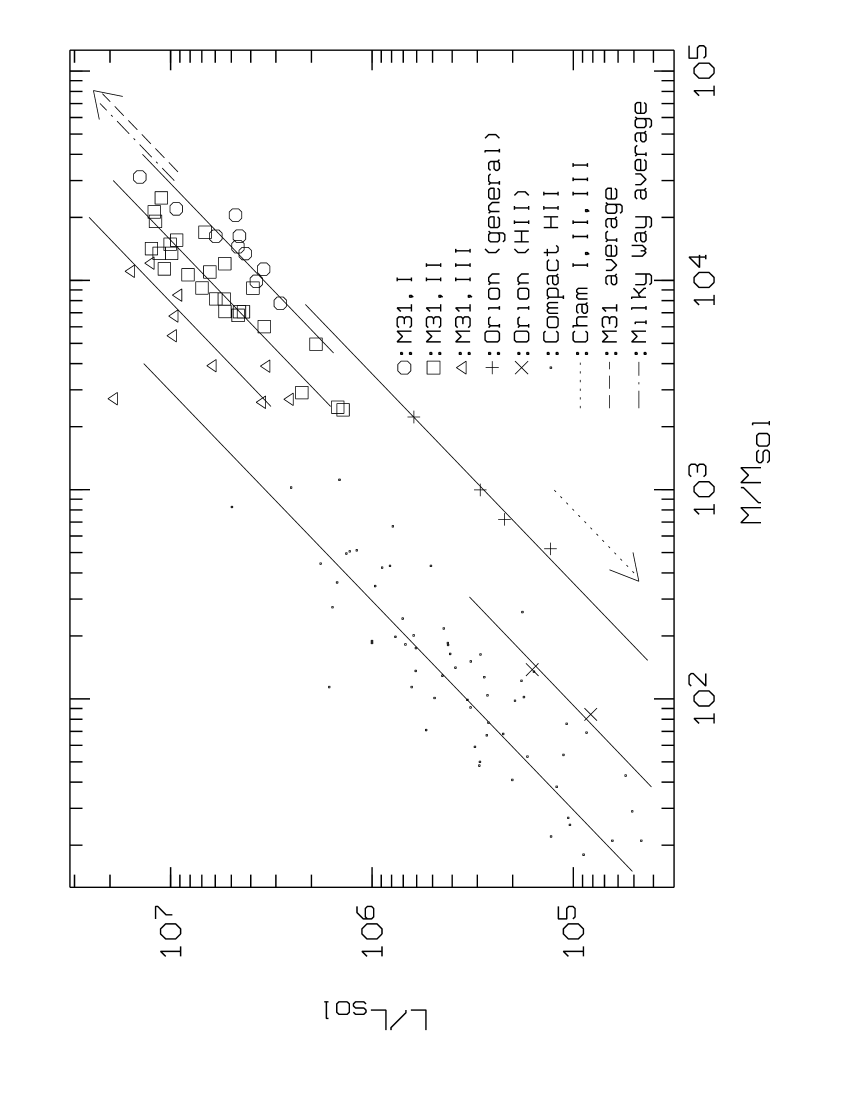
Figure 6: FIR luminosity against dust mass. The symbols refer to the three knot types and to comparison regions as indicated. For each group, the linear fit is shown by the lines, with the offsets illustrating the different $L/M$ values. For the Chameleon clouds and the whole galaxies the data values lie outside the box, thus the positions of their average lines are indicated by arrows. The values and references are given in Table 2.

Table 2: The FIR luminosity to dust mass ratio in solar units averaged for the knots and comparison objects. The data for Orion have been recalculated with our model parameters.

Objects	$L_{\rm FIR}/M_{\rm Dust}$
M 31 knots SED type I	345 $\pm$ 76
M 31 knots SED type II	642 $\pm$ 159
M 31 knots SED type III	1270 $\pm$ 311
M 31 (average)	280 $\pm$ 56
M 31 (10 kpc ring without knots)	267 $\pm$ 35
M 31 (5 kpc ring without knots)	271 $\pm$ 47
M 31 (disk, 8–12 kpc distance)	26 $\pm$ 4
M 31 (disk, 3–6 kpc distance)	45 $\pm$ 7
M 31 (central part 0.8–1.3 kpc)	145 $\pm$ 34
Orion (general) (Wall et al. (1996))	284 $\pm$ 59
Orion (H II) (Wall et al. (1996))	1070 $\pm$ 217
Compact H II regions (Chini et al. (1987))	3396 $\pm$ 264
Chameleon (Boulanger et al. Boul98 (1998))	151 $\pm$ 25
Milky Way (average) (Sodroski et al. Sod+94 (1994))	320 $\pm$ 32

In order to compare knots in M 31 and dust clouds in the Milky Way, a suitable parameterisation is required. We use the $L/M$ ratio as parameter. The advantage over using the temperature alone lies in the fact that $L/M$ accounts simultaneously for an increase of $L$ due to the warm dust and an increase of $M$ due to the cold dust. Note that the 175 $\mu$m data now allow for a reasonable estimate of the cold dust component, which was not possible from the 60 and 100 $\mu$m data alone. In the case of one single modified Planckian, $L/M$ is equivalent to using the temperature (see Eqn. 1). So far the $L/M$ ratio provides a measure for the normalized energy content of the dust. Power sources are the interstellar radiation field (ISRF) and star formation (SF) in the knots. Note that our $L/M$ ratio considers only the dust, thus it differs from previous concepts of L_FIR/M_GAS derived for galaxies, compact H II regions, and various molecular clouds and star forming regions (Chini et al. Chini et al. (1986), Chini et al. (1987), Wall et al. (1996), Boulanger et al. Boul98 (1998)). We will first consider only SF.

In Fig. 6 the FIR luminosity of each knot is plotted against its dust mass. The knots fill a continuous range in this diagram, but the three SED types are well separated. A least square fit

$$L=C\cdot M^{\rm\alpha},\\$$ (4)

yields $\alpha$ = 1.03 $\pm$ 0.10 but a different value $C$ for each SED-type. With $\alpha$ being one, $C$ is equal to the average $L/M$-ratio, listed in Table 2. Thus within each SED type the $L/M$ ratio seems to be independent of the absolute values of $L$ or $M$, which allows for a direct comparison of large and small cloud complexes via $L/M$.

In order to disentangle the power contribution of the ISRF and SF in the knots, we try to find some reasonable values for the ISRF. One can safely assume that the regions outside the rings are mainly heated by the ISRF. This is equivalent to the assumption that in M 31 the SF is confined to the three ring-like structures at radii of 5, 10 and 14 kpc which is consistent with H_α observations (Devereux et al. (1994)). As the ISRF variates along the galaxy, i.e. it is higher in the bulge region than in the outer parts (Pagani et al. Pag+99 (1999)), we have determined the $L/M$-ratios for several fields in the following regions:

• in the central bulge region (0.8-1.3 kpc)

• in the disk between 3 and 6 kpc, excluding the 5 kpc ring

• in the disk between 8 and 12 kpc, excluding the 10 kpc ring

• along the 5 kpc ring but avoiding the knots.

• along the 10 kpc ring but avoiding the knots.

The resulting average values for these regions are given in Table 2. Except for the central part, the $L/M$-ratio of the inter-ring regions are extremely low. In the rings, instead, the average value outside the knots $L/M=269$ is quite high. This might be explained by an increase of the ISRF in the ring or more likely by the assumption that the ring contains more unresolved dust clouds and/or star forming region.

Inside the knots the ISRF cannot be stronger, rather, the knots might be shielded against radiation from outside. Hence, for dust heated only by the ISRF, values between 20 and 50 are expected for the $L/M$ ratio. The power of the warm and probably also the medium knots (having $L/M$ ratios of more than 600) is therefore certainly dominated by SF. The cold knots have an average $L/M$ ratio of 345, which is still too high for a heating of the ISRF only, but the difference to the surrounding inner-ring regions is small. This can be interepreted in the way that in these sources also the ISRF plays a major role, which must then be higher in the rings than outside. However, it does not account for the whole power. Hence, even the cold knots require additional heating, which could come from a high number of low mass stars or from young massive stars. Their UV radiation, however, has to be absorbed effectively within the clouds, since signatures of a strong UV field are not observed (Cesarsky et al. (1998) and Pagani et al. Pag+99 (1999)).

10 Comparison with radio and optical tracers

The celestial coordinates of the knots have been used for identification of the sources in observations at other wavelengths. Special emphasis has been placed on the catalogue of optically identified H II regions (Pellet et al. (1978)) and the radio continuum as tracer for H II regions. We have used the 610 MHz catalogue of Bystedt et al. (Bys84 (1984)) which is flux limited and provides a list of well identified sources. In order to separate the thermal and nonthermal radio emission, maps at 2 cm or 6 cm are required but are not yet available. Furthermore, catalogues of supernova remnants (SNRs) (Dickel & D’Odorico (1984)) and dark clouds (Hodge Hod80 (1980)), and surveys of CO (Dame et al. Dam+93 (1993)) and H I (Brinks & Shane Bri84 (1984)) have been looked up for comparison. We limited our comparison to these catalogues, because they cover the complete area of M 31, where the FIR knots are situated. The results of this search are listed in column (15) of Table 1.

These tracers do not simply correlate with classification of the FIR knots. Nevertheless, some statistical trends can be recognized: A large number of our warm knots (SED types III, and also II) are identified as H II regions. This is expected, as nearly all the 60 $\mu$m point sources coincide with H II regions (Xu & Helou Xu96 (1996)). The 20 cm map of Beck et al. (Beck+98 (1998)) has been looked up and yields coincidence with nearly every knot independant of the SED type. However, the cold knots of type I are not as prominent at 20 cm as the warm knots of type III.

Figure 7: Statistical coincidence of the FIR knots with detections by other tracers separated for each SED type. The cold knots (type I) are more related to detections in H I and CO, whereas the warm knots (type III) are dominant at SNRs and H II regions. The medium knots (type II) follow more a mean distribution.

Although the optically dark dust lanes in M 31 generally match the FIR ring quite well, only a weak correlation with the dark clouds (Hodge Hod80 (1980)) is found. The high number density of these dark clouds, however, considerably increases the likelihood of finding one at any randomly picked position within our spatial resolution of 90^′′. In this respect, it appears more interesting that a number of even large dark clouds like D76, D144, D425 or D517 are not found in the 175 $\mu$m map. They probably do not have sufficient mass to provide a prominent 175 $\mu$m emission. This picture is consistent with the lack of any correlation between optical extinction maps as created by Nedialkov (Ned98 (1998)) and our FIR sources. A moderate amount of just 1 mag of visual foreground extinction already results in a dark lane.

SNRs are found close to the position of some of the knots, but they are not sufficiently coincidental to provide evidence for a correspondence. However, SNRs are only found for warm (and medium) knots with temperatures of the cold dust component above 17 K (SED types II and III). Most of the warm knots correspond with H II regions, hence they contain high mass stars, i.e. the precursors of SNRs. Therefore SNRs are also most likely to be found in warm knots.

In Fig. 7 the coincidence of the FIR knots with the other tracers is illustrated as a histogram for the three SED types. Whereas the knots of type II more or less follow the general distribution, the warm knots are more frequently represented by the SNRs and H II regions as discussed above, and the cold knots of type I correlate with detections in CO and H I.

For the southwest part of M 31, new CO observations with higher resolution and sensitivity have been presented by Neininger et al. (Nei+98 (1998)) and Loinard et al. (Loi+99 (1999)). A comparison of the knots of this area with the new CO data reveals, that all of them have a faint CO counterpart. The same will probably be the case for the other radio tracers, where so far no better data are available. The catalogues used are intensity limited. Hence, the coincidences of the FIR knots with the other tracers must not be interpreted in the way, that e.g. the warm knots do not contain any CO, but that they emit too faintly to be detected in the survey of Dame et al. (Dam+93 (1993)). On the other hand, also the cold knots do probably contain H II, but the emission is too faint to be detected. However, this does not alter the general conclusion, that the cold knots are more related to CO and H I, the warm knots more to H II.

11 Nature of the knots

What are the different types of knots? In this section we combine the information collected so far: the spatial coincidence with other tracers of known physical properties, and the $L/M$ ratio tracing the energy content and providing unbiased clues for the dominating power source. But first we have to consider the spatial extension.

11.1 Extended cloud complexes

The extension of the knots (listed in column (4) of Table 1) is significantly higher than the FWHM of point sources due to ISO’s resolution. With the adopted distance of 690 kpc the average diameter computes up to about 800 pc. Since this appears too large for a single dust cloud, the FIR knots might rather represent numerous clouds in chance projection or giant complexes of molecular clouds with associated H II regions, where the single clouds are too small to be separated within our resolution (300 pc). This consideration is supported by the work of Loinard et al. (Loi+99 (1999)). In their figures 6 e-g, they demonstrate very clearly the influence of angular resolution on the observed size of objects, which consist of several small, unresolved clouds. The additional possibility of chance projection does not alter our conclusions, so in the further discussion we consider only the case of cloud complexes.

This picture explains well the high dust masses and luminosities which are more typical for a dwarf galaxy than for a galactic complex. For example, the fairly large Orion complex in our own Galaxy, including Orion A, Orion B and $\lambda$ Ori, has a diameter of less than 300 pc, and is therefore a factor of three smaller than most of the M 31 knots. Accordingly, for the Orion complex the integrated dust mass of $\rm 2.9\cdot 10^{3}M_{\odot}$, and the combined infrared luminosity of $\rm 9.4\cdot 10^{5}L_{\odot}$ (Wall et al. (1996)) are smaller than for the M 31 knots.

11.2 Warm knots: Huge star forming complexes

The investigations provide evidence that the warm knots of SED type III represent huge complexes mainly powered by high mass star formation. The reasons are (1) the frequent spatial coincidence with H II regions (Fig. 7) and (2) the $L/M$ excess well above the ISRF traced by the rest of M31 (Fig. 6, Table 2).

This excess is similar to that of Orion’s H II regions M 42 and NGC 2024. As explained before, the knots as we see them are most probably not single dust clouds, but cloud complexes with a mixture of several dust clouds with different individual temperatures. Therefore, the derived $L/M$ value is just an average and is expected to be larger for individual clouds, reaching the range of the Galactic compact H II regions. Hence, the warm knots are very good candidates for containing not only moderate SF regions but also compact H II regions.

11.3 Cold knots: Giant molecular cloud complexes

The cold knots of SED type I represent giant molecular cloud complexes which contain at least a few star forming regions. The evidence comes from (1) the spatial coincidence with both the CO and H I detections and (2) the $L/M$ ratio (see Table 2) which is higher for the cold knots than for the rest of M 31 tracing the ISRF as discussed in Sect. 9. For comparison, the $L/M$ values for the Chameleon clouds which exhibit only low mass star formation are clearly lower and even below the average of the Milky Way. Thus, at least a moderate SF also takes place in the cold knots of M 31.

This picture might be supported by the distribution of the thermal radio continuum as tracer for ionized gas. A comparison has been performed with figures 4 and 5 of Beck et al. (Beck+98 (1998)), showing the radio continuum at 20 cm. Except for knot 23, for all cold knots in the overlapping part radio continuum radiation is present, though only weak for knots 15, 17, and 37. Unfortunately in M 31 the synchroton radiation is very strong and still dominates the radio continuum at 20 cm (Hoernes et al. Hoe+98 (1998)). It will therefore be interesting to compare the FIR knots with the new 6 cm Effelsberg survey (Berkhuijsen et al., in prep.) and a corresponding thermal radio map resulting from the decomposition of the radio continuum.

11.4 Medium knots: Mixture of warm and cold knots

The knots of SED type II do probably represent a mixture containing both high mass star forming regions and cold molecular cloud complexes. Arguments in favour of this view come from the middle position in (1) cold dust temperatures and colours and (2) $L/M$ excess and (3) the average spatial coincidence with H II regions as well as CO and H I detections.

11.5 The enigmatic knot # 23

Knot # 23 northwest of M31’s centre is by far the brightest 175 $\mu$m region of M 31. Despite its dominant 175 $\mu$m appearance, the object does hardly show up in the IRAS 12 and 25 $\mu$m HIRES maps, and gets only a little pronounced in the 60 $\mu$m map, especially when compared to the bright knots in the outer rings. At 100 $\mu$m it is clearly visible, but it is not the brightest region of M 31. This object constitutes a real puzzle, since it is not prominent at any other tracers: No radio continuum has been detected so far in this region (Braun (1990); Beck et al. Beck+98 (1998)). Only diffuse and faint H I emission can be found with no dominant feature at the position of the knot (Brinks & Shane Bri84 (1984)). The same yields for optical investigations. In Hodge (Hod80 (1980)) and Hodge (Hod81 (1981)) a lot of extinction is seen around the knot, but no specific dark cloud can be identified with the source. Whereas no CO is seen on the maps of Dame et al. (Dam+93 (1993)), new CO observations at higher resolution reveal a clumpy structure of small and faint CO sources (Nieten et al. (2000)).

With a temperature of 16.5 K, knot # 23 belongs to the cold SED type I. However, the value of $L/M=450$ is still relatively high. Between 100 $\mu$m and 175 $\mu$m the intensity increases by a factor of 2, and we expect the maximum to lie even beyond 175 $\mu$m. In this case the temperature could be lower and the mass even higher, bringing $L/M$ closer to the value of about 150 for the central part powered only by the ISRF. For this, the mass of the dust inside the measured aperture has to increase to at least $10^{5}$ M_⊙. As the Jeans limit for a single cloud with $R=10^{6}$ pc and $T=20$ K can be estimated to be about 500 M_⊙, one will have problems to explain the stability of this complex without assuming SF. Therefore, a pure heating from outside via the ISRF does not seem sufficient, but further observations in the submm will clarify this point. Additional clues will come from future observations of the thermal radio component of this region, and maybe even of the stellar population inside the knot. On the basis of the current data, also the possibility of a background object like a radio galaxy cannot be ruled out.

- (1) Baade, W., Arp, H. 1964, ApJ 139, 1027
- (2) Beck, R., Berkhuijsen, E.M., Hoernes, P. 1998, A&AS 129, 329
- (3) van den Bergh, S. 1991, PASP 103, 1053
- (4) Berkhuijsen, E.M., Wielebinski, R., Beck, R. 1983, A&A 117, 141
- (5) Boulanger, F., Bronfman, L., Dame, T.M., Thaddeus, P. 1998, A&A 332, 273
- Braun (1990) Braun, R. 1990, ApJS 72, 761
- (7) Brinks, E., Shane, W.W. 1984, A&AS 55, 179
- (8) Bystedt, J.E.V., Brinks, E., de Bruyn, A.G., et al. 1984, A&AS 56, 245
- Cesarsky et al. (1998) Cesarsky, D., Lequeux, J., Pagani, L., et al. 1998, A&A 337, L35
- Chini et al. (1986) Chini, R., Krügel, E., Kreysa, E. 1986, A&A 167, 315
- Chini et al. (1987) Chini, R., Krügel, E., Wargau, W. 1987, A&A 181, 378
- Cram et al. (1980) Cram, T.R., Roberts, M.S., Whitehurst, N.S. 1980, A&AS 40, 215
- (13) Dame, T.M., Koper, E., Israel, F.P., Thaddeus, P. 1993, ApJ 418, 730
- (14) Désert, F.-X., Boulanger, F., Puget, J.L. 1990, A&A 237, 215
- Devereux et al. (1994) Devereux, N.A., Price, R., Wells, L.A., Duric, N. 1994, AJ 108, 1667
- Dickel & D’Odorico (1984) Dickel, J.R., D’Odorico, S. 1984, MNRAS 206, 351
- (17) Dwek, E., Arendt, R.G., Fixsen, D.J., et al. 1997, ApJ 475, 565
- (18) Fich, M., Hodge, P. 1991, ApJ 374, L17
- Gillespie (1979) Gillespie, A.R. 1979, MNRAS 188, 481
- (20) Haas, M., Lemke, D., Stickel, et al. 1998, A&A 338, L33
- (21) Habing H.J., Miley G., Young E., et al. 1984, ApJ 278, L59
- (22) Hildebrandt, R.H. 1983, QJRAS 24, 267
- (23) Hodge, P. 1980, AJ 85, 376
- (24) Hodge, P. 1981, Atlas of the Andromeda galaxy, University of Washington Press 1981
- Hodge (1990) Hodge, P. 1990, ’The Andromeda Galaxy, Kluwer Academic Publishers, Dordrecht, 1992
- (26) Hoernes, P., Berkhuijsen, E.M., Xu, C. 1998, A&A 334, 57
- Kessler et al. (1996) Kessler, M.F., Steinz, J.A., Anderegg M.E., et al. 1996, A&A, 315, L27
- Krügel & Chini (1994) Krügel, E., Chini, R. 1994, A&A 287, 947
- Lemke et al. (1996) Lemke, D., Klaas, U., Abolins J., et al. 1996, A&A 315, L64
- Loinard & Allen (1998) Loinard, L., Allen, R.J. 1998, ApJ 499, 227
- Loinard et al. (1996) Loinard, L., Dame, T.M., Koper, E., et al. 1996, ApJ 469, L101
- (32) Loinard, L., Dame, T.M., Heyer, M.H., Lequeux, J., Thaddeus, P. 1999, A&A 351, 1087
- (33) Nedialkov, P. L. 1998, Ph.D. Thesis, Sofia University
- Nieten et al. (2000) Nieten, Ch., Neininger, N., Guelin, M. et al., 2000, The Interstellar Medium in M31 and M33, Proceedings of the WE-Heraeus-Seminar, in press
- (35) Neininger, N., Guelin, M., Ungerechts, H., Lucas, R., Wielebinski, R., 1998, Nat 395, 871
- (36) Pagani, L., Lequeux, J., Cesarsky, D., et al. 1999, A&A 351, 447
- Pellet et al. (1978) Pellet, A., Astier, N., Viale, A., et al. 1978, A&AS 31, 439
- Ristorcelli et al. (1998) Ristorcelli, I., Serra, G., Lamarre, J.M., et al. 1998, ApJ 496, 267
- Ristorcelli et al. (1999) Ristorcelli, I., Serra, G., Lamarre, J.M., et al. 1999, Solid Interstellar Matter: The ISO Revolution, d’Hendecourt L., Joblin C., Jones A. (eds.), EDP Sciences and Springer-Verlag, 49
- (40) Sodroski, T.J., Bennett, C., Boggess, N., et al. 1994, ApJ 428, 638
- Sofue et al. (1981) Sofue, Y., Kato, T. 1981, PASJ 33, 449
- (42) Toth, V., Hotzel., S., Lemke, D., et al., 2000, submitted to A&A
- Wall et al. (1996) Wall,W.F., Reach, W.T., Hauser, M.G. et al. 1996, ApJ 456, 566
- Walterbos & Schwering (1987) Walterbos, R.A.M., Schwering, P.B.W. 1987, A&A 180, 27
- (45) Xu, C., Helou, G. 1996, ApJ 456, 152