Properties of galaxy halos in Clusters and Voids

Abstract

We use the results of a high resolution N-body simulation to investigate the rôle of the environment on the formation and evolution of galaxy-sized halos. Starting from a set of constrained initial conditions, we have produced a final configuration hosting a double cluster in one octant and a large void extending over two octants of the simulation box. In this paper we concentrate on gravitationally bound galaxy-sized halos extracted from these two regions and from a third region hosting a single, relaxed cluster without substructure. Exploiting the high mass resolution of our simulation ($m_{body}=2.1\times 10^{9}h^{-1}M_{\odot}$), we construct halo samples probing more than 2 decades in mass, starting from a rather small mass threshold: $5\times 10^{10}h^{-1}M_{\odot}\leq M$. We present results for two statistics: the relationship between 1-D velocity dispersion $\sigma_{v}$  and mass $M_{0}$  and the probability distribution of the spin parameter $P(\lambda)$, and for three different group finders. The $\sigma_{v}-M_{0}$  relationship is well reproduced by the Truncated Isothermal Sphere (TIS) model introduced by Shapiro et al. (1999), although the slope is different from the original prediction. A series of $\sigma_{v}-M_{0}$  relationships for different values of the anisotropy parameter $\beta$, obtained using the theoretical predictions by Łokas & Mamon (2001) for Navarro et al. (1996, 1997) density profiles are found to be only marginally consistent with the data. Using some properties of the equilibrium TIS models, we construct subsamples of fiducial equilibrium TIS halos from each of the three subregions, and we study their properties. For these halos, we do find an environmental dependence of their properties, in particular of the spin parameter distribution $P(\lambda)$. We study in more detail the TIS model, and we find new relationships between the truncation radius and other structural parameters. No gravitationally bound halo is found having a radius larger than the critical value for gravithermal instability for TIS halos ($r_{t}$  $\geq 34.2r_{0}$, where $r_{0}$ is the core radius of the TIS solution). We do however find a dependence of this relationship on the environment, like for the $P(\lambda)$ statistics. These facts hint at a possible rôle of tidal fields at determining the statistical properties of halos.

1 Introduction

One of the distinguishing features of any scenario for the formation of the Large Scale Structure of the Universe within the Cold Dark Matter (CDM) cosmological model is represented by the hierarchical clustering paradigm for the assembly of gravitationally bound structures (White 1996, 1997). In its simplest form, the idea of hierarchical clustering implies the fact that the growth of halos proceeds by accretion of smaller units from the surrounding environment, either by infall (Gunn & Gott 1972) or by a series of of “merging“ events (White & Rees 1978), whereby the subunits are accreted in a discontinous way, or (more likely) by a combination of the two. In the first case the typical halo profiles evolve adiabatically, while in the merging scenario each merging “event” will induce some transients in the characteristic properties which in turn will induce some evolution in the typical profiles, after the subunits have been accreted and destroyed. In either case, one expects that relaxation processes should drive the evolution towards a quasi-equilibrium state on a dynamical timescale, a state characterized by relationships among global quantities related to the halo, like its mass, density, velocity dispersion $\sigma_{v}$, and possibly others. Recently a considerable attention has been devoted to the study of one of these relationships: the radial dependence of the (spherically averaged) density, also known as the density profile. Unfortunately the density profile is a very difficult tool to use when trying to characterize the statistical properties of halo populations, because the predictions of different models of halo formation differ only in the behaviour in the central parts, where the statistics is typically poor. Less attention has been paid to another global quantity, namely the velocity dispersion and to its relationship with other global quantities, like the mass. The velocity dispersion enters the second-order Jeans equation, while the density profile is described by the zeroth-order Jeans equation (Binney & Tremaine 1987). For this reason it contains different physical information than the density profile. Recently Bryan & Norman (1998) have looked at the $\sigma_{v}-M_{0}$  relationship for clusters, and they find a good agreement with the standard, singular isothermal sphere model as far as the slope of the relationship is concerned. Also Knebe & Müller (1999) looked at this relationship, using a different code. Halo equilibrum models make predictions about the $\sigma_{v}-M_{0}$  relationship, but these are difficult to compare with observations, because some of the involved quantities (e.g. the velocity dispersion itself) are not directly deducible from observations. They can however be studied with N-body simulations, and one of the purposes of this paper will be to show that the $\sigma_{v}-M_{0}$  relationship can be used to discriminate among different halo equilibrium models.
A second problem we will study concerns the dependence of halo properties on the environment within which they form. In both the hierarchical clustering scenarios mentioned above one could imagine that the properties of the halos do depend on the environment. For instance, the dynamics of the infall process could be affected by the average overdensity of the environment within which the halo grows (Gunn 1977), or by its shear (Buchert et al. 1999; Takada & Futamase 1999). Also typical quantities related to the merging, like the frequency of merging events, could intuitively be affected by the average density of the environment, at least for galaxy-sized halos forming within clusters. High resolution N-body simulations (e.g. Moore et al. 1999) show that most of the galaxies lying in the central (i.e. virialised) parts of clusters do not easily reach a velocity larger than the escape velocity: so, they are bound to the cluster for the largest part of their evolutionary history, and consequently form in an overdense environment. It would then be interesting to try to understand whether there are systematic differences between halos forming in clusters and in voids.
Some of these issues have been recently discussed in the literature. Lemson & Kauffmann (1999) have analysed the dependence of various statistical properties, including the spin probability distribution, on the environment, and found no evidence for any dependence apart for the extent of the mass spectrum. They divide their halos in groups according to the overdensity of the environment within which they are found, and show that the scatter diagrams between different quantities are indistinguishable among the different groups. In the present study, we follow a different strategy. We study a simulation obtained from a constrained set of initial conditions, in order to get a few clusters (and, in particular, a double cluster) and a large void within the same simulation box. We then extract our halos from three spatially disjoint regions: one containing a double cluster, a second one contaning a single cluster a third one containing the void. This is in some sense complementary to the procedure which Lemson & Kauffmann seem to have followed, because our halos are grouped according to the spatial distribution, rather than according to the overdensity, so they are grouped according to the environment within which they form.
Very recently Gardner (2000) presented a study of the spin probability distribution for 6 different cosmological models and environments. He finds a difference between the distributions of halos resulting from recent mergers and halos which did not experience mergers, almost independent of the environment within which they form. This could have significant consequences for the construction of merger histories, and, ultimately, for the semi-analytical modelling of galaxies. Similar results have been recently obtained by Vitvitska et al. (2001).
The plan of the paper is as follows. In section  2 we describe the numerical setup of the simulations and the algorithm adopted to identify halos. In section  3 we describe the halo equilibrium models with which we compare the results of our simulation, and in section  4 we show the results of this comparison and discuss their physical interpretation. Finally, in the conclusions we summarize our results and suggest some directions for future studies.

In the following we will always assume a $\Omega=1$ Standard Cold Dark Matter model, with a Hubble constant $H_{0}=100h\,{\rm Km\,s^{-1}\,Mpc^{-1}}$, and $h=0.5$. All lengths, unless explicitly stated, are assumed to be comoving.

2 Simulations

The simulation from which the data have been extracted has been performed using FLY (Becciani et al. 1997, 1998) a parallel, collisionless treecode optimised for Shared Memory and/or clustered computing systems. FLY deals with periodic boundary conditions using a standard Ewald summation technique (Hernquist et al. 1991). The algorithm adopted is the octal-tree algorithm of Barnes & Hut (Barnes & Hut 1986), with some modifications (“grouping” of cells belonging to the lists of nearby particles, Barnes 1987) during the phase of tree walking. These changes have a negligible impact on the overall numerical accuracy, as shown elsewhere (Becciani et al. 2000), but they have a strong positive impact on parallel peformance and scaling.
We have performed two simulations starting from the same initial conditions. In both cases the underlying cosmological model is a Standard Cold Dark Matter (SCDM), with $\Omega_{0}=1,\sigma_{8}=0.9$. The main reason for this choice lies in the fact that the specific prediction for the $\sigma_{v}-M_{0}$  statistics we consider in the next sections were done for this particular cosmological model. We plan to extend our work to other cosmological models in future work.
Each simulation used $256^{3}$ particles, and the box size was 50$h^{-1}$Mpc, so that the mass of each particle is $m_{part}=2.07\times 10^{9}$ $h^{-1}{\rm M}_{\odot}$. The simulations were designed to study the evolution of a Coma-like cluster, and for this purpose constrained initial conditions were prepared, changing only the softening length, which was fixed to $\epsilon=10$ $h^{-1}$kpc  and $5$ $h^{-1}$kpc, respectively. As far as the results presented in this paper are concerned, there are no differences among these two simulations, so for the rest of this paper we will concentrate only on the simulation with the largest softening length, which we designate in the following as 16ML_1.

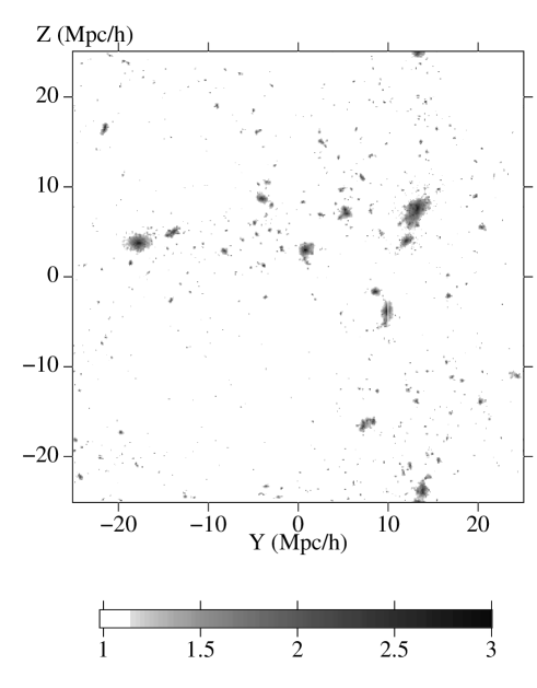
Figure 1: Snapshot of the simulation box at the end of the simulation. The scale of grey corresponds to density in logarithmic units. The large void is clearly seen in projection extending over the lower left octant.

Constrained initial conditions were prepared using the implementation of the constrained random field algorithm of Hoffman & Ribak (1991) by van de Weygaert & Bertschinger (1996). We took the same initial conditions adopted in one of the simulations from the catalogue of van Kampen & Katgert (1997). More specifically, we constrain the initial conditions to have a peak at the centre of the simulation box, with height $3.04\sigma$, Gaussian smoothed at a scale of $6h^{-1}$ Mpc, and a $-2\sigma$ void centered at $(15,0,-10)$. The final configuration is shown in Figure 1. In order to study the environmental dependence of the properties of galaxy-sized halo populations, we selected three regions within the computational box, which we call DOUBLE, SINGLE and VOID. All the three are cubical with centers and sizes as specified in Table 1. The DOUBLE region hosts a double cluster, with two large parts in the act of merging by the end of the simulation (see Fig. 2). The SINGLE region hosts a more relaxed cluster without any apparent substructure. Finally, we have included in the analysis a significantly underdense region, the VOID, which is more extended than the former two, so as to contain enough halos to allow a reasonable statistics.

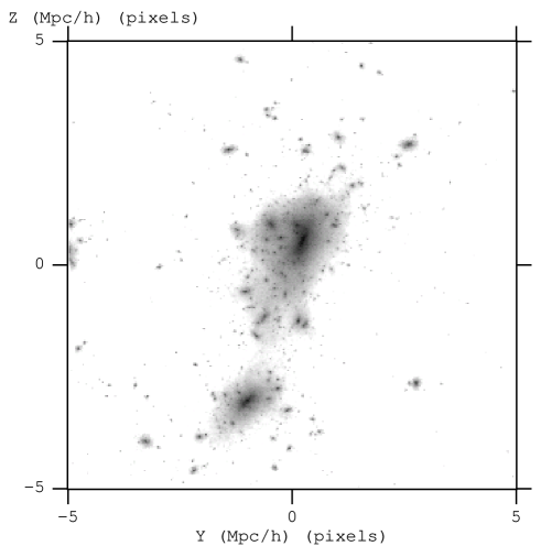
Figure 2: The region of the DOUBLE cluster.

Table 1: Properties of the analyzed regions.

Region	$x$	$y$	$z$	$L$	Number of halos
DOUBLE	15	12.5	7.5	10	827
SINGLE	12	-18	4	10	786
VOID	-10	-10.	-10.	20	609

All lengths are in $h^{-1}$Mpc. From left to right, columns are as follows: label of the region, x,y,and z coordinate of its center, size of the region, total number of halos found.

2.1 Finding halos

Various methods have been devised to extract halos from the outputs of N-body simulations. Some of these methods make use only of particle positions, like the standard Friends-Of-Friends (herefater FOF) and the various versions of the Adaptive FOF, while others take into account also particle velocities (e.g. $SKID$, Governato et al. 1997) and/or environmental properties like local densities (like HOP, Eisenstein & Hut 1998). Most of the results we will present later have been obtained using $SKID$ because it selects gravitationally bound groups of particles. In short, $SKID$ first builds catalogues of groups using a standard FOF algorithm, selecting only particles lying within regions whose density is larger than a critical value $\delta_{crit}$. It then computes the escape velocity of each particle and discards those particles having a rms velocity larger than the escape velocity. This “pruning” procedure should then leave only those particles which are actually bound to the group, discarding those “background” particles which find themselves by accident at a given time within it. The initial linking length of the FOF phase determines the approximate size of the groups we are considering. We assumed a linking length of $100h^{-1}{\rm kpc}$, corresponding to the typical size of a galaxy-sized object at the present epoch. The softening length for the calculation of the gravitational potential was assumed to be the same as in the simulation, and the critical density $\delta_{crit}$ was set equal to $178/(1+z)$, the value for nonlinear collapse in the Gunn & Gott collapse model, so that only particles from genuinely nonlinearly collapsed shells should be included.
Following a suggestion of the anonymous referee, we have also adopted two more halo finders to check the robustness of the results: an Adaptive FOF method devised by van Kampen & Katgert (1997) and a modified version of SKID  which should avoid the problems posed by the original version. This particular AFOF halo finder selects only those haloes that are virialized, by specifically testing for virialization. Concerning the second method, we have modified SKID  only in that part which engenders the input group list which is subsequently “pruned” of the non-gravitationally bound particles: in place of a standard FOF (as in the original version of SKID) we have adopted HOP(Eisenstein & Hut 1998) as input group finder. As we will see later, some of the relationships we find do depend on the group finder adopted, but those relationships holding for the equilibrium TIS halos are not affected by this. All the results we present in the following are for the final redshift of the simulation, $z=0.0047$, unless otherwise stated.

3 Halo equilibrium models

The internal properties of halos formed by gravitational collapse can be described by looking at correlations among different physical quantities. The density profile has often been used to study the properties of relaxed, virialised halos, particularly since the findings by Navarro, Frenk, & White (1996) that this profile has a universal character when expressed in dimensionless units. However, the density profile can be reliably determined only for halos having enough particles in each shell to minimise the statistical fluctuations. For instance, Navarro et al. (1997) considered only 8 halos extracted from a low resolution simulation and re-simulated with a higher mass resolution.
Typical N-body simulations on cluster scales tend to produce a large amount of halos, whose density profile can not be reliably determined, because each of them contains on average less than $10^{5}$ particles. For this reason we have chosen to study relationships involving global halo properties. This choice is not free from potential problems: systematic biases can be introduced by the particular group finder adopted. Consider for instance SKID, which works by stripping out gravitationally unbound particles from halos builded using FOF: the group catalogues so produced tend to be more biased towards less massive halos than catalogues produced using FOF. We have then decided to adopt three different group finders, in order to be able to understand the role of these systematic factors. We have also considered two different statistics to characterize the properties of dark matter halos, and particularly their equilibrium properties at the end of the simulation: the internal 1-dimensional velocity dispersion - mass relationship ($\sigma_{v}-M_{0}$ ) and the spin probability distribution ${\rm P}(\lambda)$. Theoretical predictions concerning both of them are available in the literature. In particular, we will compare the results from our N-body simulations with four models: the Standard Uniform Isothermal Sphere (SUS) (see e.g. Padmanabhan 1993, chap. 8 for a detailed treatment), the Truncated Isothermal Sphere models (TIS) recently introduced by Shapiro et al. (1999), the “peak-patch” (PP) Montecarlo models by Bond & Myers (1996a), and some models derived from the Navarro et al. (1996, 1997) (hereafter NFW) density profiles. The first two models predict a $\sigma_{v}-M_{0}$  relationship given by:

$$\sigma_{v}=c_{f}\,{\rm M}_{12}^{1/3}\left(1+z_{coll}\right)^{1/2}h^{1/3}\,{\rm Km\,s^{-1}}$$ (1)

where the subscript $f\equiv SUS\,{\rm or}\,TIS$, while for the PP model the relation is given in Bond & Myers (1996b):

$$\sigma_{v}=c_{PP}\,{\rm M}_{12}^{0.29}\left(1+z_{coll}\right)^{1/2}h^{1/3}\,{\rm Km\,s^{-1}}$$ (2)

In the equations above ${\rm M}_{12}$ is the mass in units of $10^{12}\,{\rm M}_{\odot}$ and $z_{coll}$ is the collapse redshift. The coefficients for these cases are given by

$$c_{SUS,TIS,PP}=(71.286,104.69,117.60)$$ (3)

respectively. We restrict our attention to these four models because the physical ingredients which enter in their formulation are very different, and encompass a sufficiently wide range among all the possible nonlinear collapse and virialization mechanisms. This wide choice reflects our generally poor level of understanding of the nonlinear physics of gravitational collapse, of its dependence on the local environment and on other properties like the merging history of the substructures.
The SUS model is based on the spherical nonlinear collapse model (Gunn & Gott 1972). In this model the collapse towards a singularity of a spherically simmetric shell of matter in a cosmological background is halted when its radius reaches a value of half the maximum expansion radius. The velocity dispersion is then fixed by imposing the condition of energy conservation, which must hold in the case of collisionless dark matter as that envisaged here. The TIS model also considers the highly idealized case of a spherically symmetric configuration, but assumes that the final, relaxed system is described by an isothermal, isotropic distribution function and that the density profile is truncated at a finite radius. Shapiro et al. (1999) have shown that this configuration could arise from a top-hat collapse of an isolated spherical density perturbation if, as shown by Bertschinger (1985), the dimensionless region of shell crossing almost coincides with the region bounded by the outer shock in a ideal gas accretion collapse with the same mass (in a $\Omega=1$ CDM model). The truncation radius is then assumed to coincide with the region of shell crossing, and this allows them to specify completely the model.
The peak-patch models introduced by Bond & Myers (1996a) are more general than the SUS model, in that they include a more realistic collapse model where deviations from spherical symmetry are taken into account. The density perturbation is approximated as an axisymmetric homogeneous spheroid. Coupling between the deformation tensor and the external and internal torques are consistently taken into account up to a few first orders, and Montecarlo realizations are used to build up catalogues of halos. These have been compared with the N-body simulations of Couchman (1991) in order to properly normalize the statistics. Note that eq. 2 is a best-fit relationship and holds for a range of halo mass ($2.5\times 10^{14}\leq M_{h}\leq 5\times 10^{15}{\rm M}_{\odot}$) much larger than that considered here. Nonetheless, we include it into our comparison because the physical model it is based on is significantly different from the other models we consider.
Finally, we have considered models for the $\sigma_{v}-M_{0}$  statistics consistent with the NFW density profile, which were recently derived by Łokas & Mamon (2001) solving the second order Jeans equation:

$$\frac{1}{\rho}\frac{\rm d}{{\rm d}r}(\rho\sigma_{\rm r}^{2})+2\beta\frac{\sigma_{\rm r}^{2}}{r}=-\frac{{\rm d}\Phi}{{\rm d}r}\ ,$$ (4)

where $\beta=1-\sigma_{\theta}^{2}(r)/\sigma_{\rm r}^{2}(r)$ quantifies the anisotropy of the velocity dispersion. For a NFW density profile we have:

$$\rho_{NFW}(r)\equiv\rho_{NFW}(s)=\frac{\rho_{c}^{0}c^{2}g(c)}{3}\cdot\frac{1}{s\left(1+cs\right)^{2}}$$ (5)

$$\Phi_{NFW}(s)=-\frac{GM_{VIR}}{r_{VIR}}\cdot g(c)\frac{\ln\left(1+cs\right)}{s}\,$$ (6)

where we have defined: $r_{VIR},M_{VIR}$ as the virialisation radius and mass, respectively, $s=r/r_{VIR}$, $c=c(M,z)$ is the concentration parameter and: $g(c)=1/(\ln(1+c)-c/(1+c))$. Eq. 4 can be solved by quadrature, and the solution finite in the limit $r\rightarrow\infty$ is:

$$\frac{\sigma_{\rm r}^{2}}{V_{v}^{2}}(s,\beta={\rm const}) = g(c)(1+cs)^{2}s^{1-2\beta}$$ (7)

$$\times \int_{s}^{\infty}\left[\frac{s^{2\beta-3}\ln(1+cs)}{(1+cs)^{2}}-\frac{cs^{2\beta-2}}{(1+cs)^{3}}\right]{\rm d}s.$$

Note that we have always chosen as critical treshold for our group finders the virialisation overdensity ($\delta\geq\delta_{crit}=178$), so the quantities $r_{VIR},M_{VIR}$ are the actual radius and mass found by the group finders for each halo.
In order to make use of eq. 7 we have yet to specify the dependence of the concentration parameter on the mass at the final redshift: $c=c(M,z=0)$. We adopt the relationship provided by Bullock et al. (2001), by running their code CVIR for the relevant cosmological model. In the mass range we are interested to ($5\times 10^{10}\leq M/M_{\odot}\leq 5\times 10^{13}$) we find a power law fit: $c(M,z=0)=472.063\times M^{-0.127\pm 0.01}$. Finally, in order to make a proper comparison with the quantity computed by the group finder, we evaluate the mass averaged velocity dispersion:

$$\sigma_{v}^{2}=\frac{4\pi\int_{0}^{1}\sigma_{v,NFW}^{2}(s)\rho(s)s^{2}ds}{M(1)}$$ (8)

where we have defined:

$$\sigma_{v,NFW}^{2}=\sigma_{r}^{2}+\sigma_{\theta}^{2}=(2-\beta)\sigma_{r}^{2}$$

and:

$$M(1)=4\pi\int_{0}^{1}\rho(s)s^{2}ds$$

4 Statistical Properties

4.1 The $\sigma_{v}-M_{0}$  relation

In Figure 3 we show plots of the final $\sigma_{v}-M_{0}$  relationship for galaxy-sized halos in the DOUBLE, SINGLE and VOID regions, respectively, obtained using SKID. The most striking difference is probably the different character of halos in the VOID region when compared with the clustered regions. Halos in VOID have a much smaller dispersion around the mean than halos in the clustered regions, and the distribution is almost symmetric with respect to the best fitting approximation. Halos in the DOUBLE region have a larger dispersion and they do show an asymmetry in the distribution around the best fit solution, i.e. an excess of low mass halos at low $\sigma_{v}$. The latter point is useful to understand the potential systematic effects introduced by a particular group finder. In Figure 4 we show the $\sigma_{v}-M_{0}$  relationship for the DOUBLE region obtained by using the two other group finders mentioned above. As is evident, the excess of low-mass halos is only an artifact introduced by SKID, which makes use of a FOF  algorithm to build up an input list of groups. The main results of the next sections, however, do not depend on the particular group finder adopted, because we will select subsamples of halos which can be regarded as equilibrium TIS halos, and for them the slope of the $\sigma_{v}-M_{0}$  relationship is independent of the particular group finder initially adopted.
A more important difference is evident from a comparison between clustered and void regions. Halos in VOID have a larger mass extent (a property already noted by Lemson & Kauffmann 1999) and also the slope of the $\sigma_{v}-M_{0}$  relation seems to be larger than for the other two cases.
In Figure 5 we show a comparison with some theoretical predictions for NFW density profiles. In order to apply eqs. 6, 7 we have still to specify a relationship between the virial radius and the corresponding mass, which enters into eq. 6. We do this by fitting a power law relationship to the data obtained from the simulations (Figure 7), which shows that the slope depends signficantly on the environment. As is evident from Figure 5, none of the models fits adequately the data. Note that there is only a slight difference bewteen isotropic ($\beta=0$) and anisotropic ($\beta=0.5$) models. Only if we allow for an unrealistically low value of the slope of the $r_{VIR}-M_{VIR}$ relationship we get a limited agreement for the DOUBLE cluster, but not for the other two regions.
The slopes of the $\sigma_{v}-M_{0}$  relationship for different regions and using different group finders seem to be consistent with each other, within the errors (Table 2). None of the theoretical models we are considering, however, seems to offer a good fit for all the cases. The TIS model seems to give a good fit for the DOUBLE region and for the SKID  group finder, but when we use the modifed SKID  group finder, which produces a sample over a more extended mass interval, we see that the original TIS model does not offer a good fit (Figure 4).

Note that the rms uncertainty of $\sigma_{v}$  in Figures 3-7 is less than 30 Km/sec, a value much lower than that found by Knebe & Müller (1999) in their simulations (see their Fig. 3). We believe that this is a consequence of the larger mass and force resolution of our simulation, and also of the use of a larger dynamic range than adopted by previous authors.

Generally speaking, a power-law seems to offer a good fit for all the three regions (although with different ranges for the three regions), but in order to determine the slope one must probably go a step further in modelling the physical state of these halos. In the next section we will explore in more detail the properties of TIS halos and we will focus our attention on their statistical properties.

Table 2: Least-square best fit parameters for $\sigma_{v}$  relationship.

Region	$\alpha$	$\Delta\alpha$	$c_{0}$		Method
DOUBLE	0.38	0.08	74.13		SKID
	0.39	0.05	87.74		SKID with HOPinput
	0.42	0.07	72.48		AFOF
	0.42	0.03	82.16		TIS selected halos
SINGLE	0.35	0.04	80.28		SKID
	0.37	0.04	82.15		SKID with HOPinput
	0.42	0.07	71.22		AFOF
VOID	0.39	0.04	86.81		SKID
	0.40	0.04	89.43		SKID with HOPinput
	0.45	0.05	63.12		AFOF
	0.38	0.02	88.60		TIS selected halos

$\alpha,c_{0}$ are the fitting parameters of a power law fit of the form: $\sigma_{v}=c_{0}M_{12}^{\alpha}$, $\Delta\alpha$ is the rms error associated with $\alpha$.

Figure 3: 1-D velocity dispersion versus mass for halos extracted from the three regions. The three fitting curves corrsond to the three cases considered in the text: Truncated Isothermal Sphere (continuous line), Bond & Myers 1996 (dotted line), Standard Uniform Sphere (dashed line). Note the larger mass extent for halos in the VOID. In all the cases, the slope is larger than predicted by models, although within clusters the statistical uncertainty is large.

Figure 4: 1-D velocity dispersion versus mass for the DOUBLE cluster region, halos selected using the AFOF and modified SKID  with HOPinput group finders. The same parameters adopted for SKID  in Figure 3 are adopted. The best fit power law for the plot in the upper figure has a slope: $\alpha=0.039\pm 0.05$.

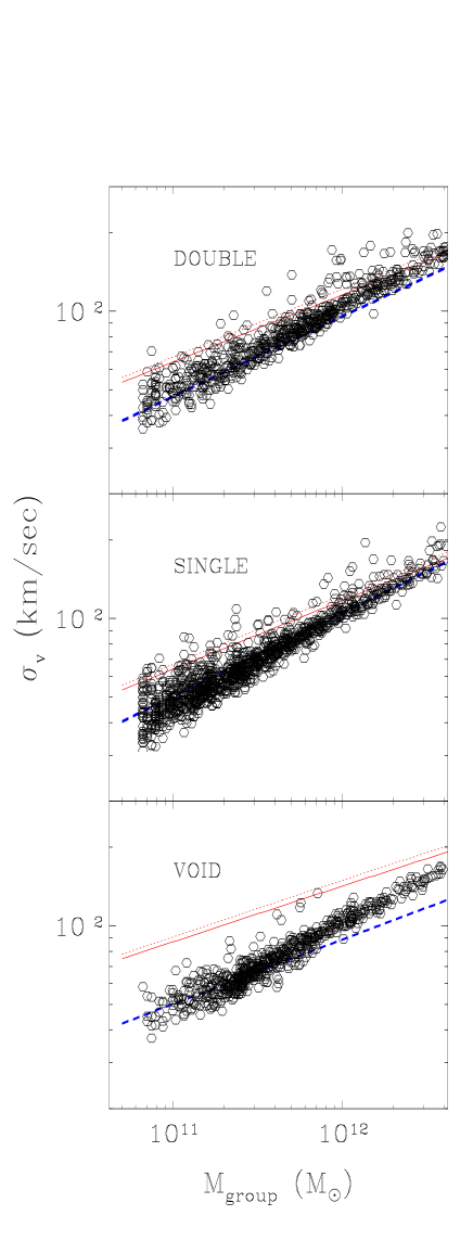
Figure 5: The $\sigma_{v}-M_{0}$  relationship for three models based on the NFW density profile. Continous line: $\beta=0$, slope of the $r_{VIR}-M_{VIR}$ given by $\alpha=\alpha_{mean}$. Dotted line: $\beta=0.5,\alpha=\alpha_{mean}$. Dashed line: $\beta=0,\alpha=\alpha_{mean}-\Delta\alpha$ (i.e. the 1$\sigma$ limit).

4.2 Comparison with the Truncated Isothermal Sphere model

We will now consider the possibility of obtaining a reasonable fit of the $\sigma_{v}-M_{0}$  relationship by modifying the minimum-energy TIS model. We will then present here some more features of this model.
Following Shapiro et al. (1999), the TIS solution is obtained by imposing a finite truncation radius $r_{t}$  on an isothermal, spherically symmetric collisionless equilibrium configuration. Shapiro et al. define a typical radius:

$$r_{0}=\frac{\sigma_{v}}{\left(4\pi G\rho_{0}\right)^{1/2}}$$ (9)

where $\rho_{0}$ is the central density (TIS models are non-singular). Combining the Poisson and the Jeans’ equilibrium equations, and making the hypothesis of isothermality for the distribution function, they obtain an equation for the dimensionless density (see Shapiro et al. 1999, eq. 29):

$$\frac{d}{d\zeta}\left(\zeta^{2}\frac{d(\ln\tilde{\rho})}{d\zeta}\right)=-\tilde{\rho}\zeta^{2}.$$ (10)

where we have used the definitions:

$$\tilde{\rho}=\displaystyle{\frac{\rho}{\rho_{0}}},\qquad\zeta=\displaystyle{\frac{r}{r_{0}}},$$

Shapiro et al. have shown that nonsingular solutions of eq. 10 form a one-parameter family depending only on $\zeta_{t}=r_{t}/r_{0}$. The total mass is then given by:

$$M_{0}=M(r_{t})=\int^{r_{t}}_{0}4\pi\rho(r)r^{2}d\,r=4\pi\rho_{0}r_{0}^{3}\tilde{M}(\zeta_{t})$$ (11)

where we have defined a dimensionless total mass:

$$\tilde{M}(\zeta_{t})=\frac{1}{r_{0}}\int_{0}^{r_{t}}dr{\rho\over\rho_{0}}\bigg{(}{r\over r_{0}}\bigg{)}^{2}$$

We follow further Shapiro et al. (1999, eq. 41) and write the virial theorem for a collisionless truncated isothermal sphere:

$$0=2K+W+S_{p},$$ (12)

where: $K=M_{0}\langle v^{2}\rangle/2\equiv\left(3/2\right)M_{0}\sigma_{v}^{2}$ and $S_{p}$ is the surface pressure term. In the Appendix we show that, after some simple algebra, starting from eq. 12 one obtains the following relation:

$$\frac{GM_{0}}{r_{t}\sigma_{v}^{2}}=\frac{3\tilde{M}(\zeta_{t})-\tilde{\rho}(\zeta_{t})}{\zeta_{t}\Psi(\zeta_{t})}\tilde{M}(\zeta_{t})\equiv\Phi(\zeta_{t})$$ (13)

The function $\Psi(\zeta_{t})$ is specified in the Appendix.
We have already seen that a power-law fit describes well the $\sigma_{v}-M_{0}$  relationship. Then from eq. 13 we deduce that also the truncation radius $r_{t}$  has a power -law dependence on the total mass: $r_{t}\propto c(\zeta_{t})M_{0}^{1-2\alpha}$. Using the values of $\alpha$ from Table 2 we see that the slope of this relationship should lie within the range 0.22-0.3, i.e. it should be quite small. In Figure 7 we plot $r_{t}$ as a function of $M_{0}$. The best-fit values we find for the slope are inconsistent with the predictions from the $\sigma_{v}-M_{0}$  relationship.
The right hand side of equation 13 depends only on the dimensionless truncation radius $\zeta_{t}$, which in the minimum-energy TIS solution of Shapiro et al. (1999) should be fixed to $\zeta_{t}=29.4$. The function $\Phi(\zeta_{t})$ has a singularity at $\zeta\approx 0.97$, where the denominator goes to zero (Figure 8). However, we are interested in the region $\zeta_{t}>1$, where the truncation radius is at least comparable to the core radius. As is clear from Fig. 10, the function has minimum at $\zeta\approx 59.5$.

Figure 6: The truncation parameter $\zeta_{t}$ as a function of group’s mass.

Figure 7: Relationship betwen truncation radius and mass. Data are fitted using a power-law relationship: $r_{t}=cM^{\alpha}$. Least-squares fit values are: $c_{SINGLE}=1.0789\times 10^{-1},\alpha_{SINGLE}=0.2637\pm 0.1335;c_{VOID}=2.7989\times 10^{-3},\alpha_{VOID}=0.3816\pm 0.0789;c_{DOUBLE}=7.3451\times 10^{-2},\alpha_{DOUBLE}=0.2791\pm 0.1193$.

We will then look for solutions in the interval $2.91\leq\zeta_{t}\leq 59.5$. Within these limits the function $\Phi(\zeta)$ is monotonically decreasing and the solution of eq. 13 is certainly unique. Note that the TIS solution is unstable for $\zeta_{t}>34.2$ (Shapiro et al. 1999; Antonov 1962; Lynden-Bell & Wood 1968), so our choice of the upper limit will allow us to verify a posteriori this prediction. Equation 13 can be inverted w.r.t. $\zeta_{t}\,$  given the left-hand side, because for each group all the quantities in the left-hand side are computed by the group finder. As for the truncation radius $r_{t}$ we adopt the groups’ radius as computed by SKID, which coincides with the virial radius $r_{VIR}$.
An interesting feature of the TIS solution, which is evident from Figure 8, is that in order to invert eq. 13 to find $\zeta_{t}\,$, the value of the left-hand side must lie within a rather small range of values: $2.75\leq GM_{0}/r_{t}\sigma_{v}^{2}\leq 4.56$. As we can see from Figure 9 for the case of the DOUBLE region, this is not the case for all the halos, even for those halos closely verifying the $\sigma_{v}-M_{0}$  relationship. For instance, out of 827 halos identified by SKID  within the DOUBLE region, only 382 lie within the region for which eq. 13 can be inverted. For those halos for which eq. 13 can be inverted, we are able to determine $\zeta_{t}\,$  and to compare it with the predictions of the minimum-energy TIS model. The results of this exercise give us some insight into the properties of these halos. In Figure 6 we plot the relationship between $\zeta_{t}\,$  and the mass for halos in the VOID and DOUBLE region (the behaviour of halos in the SINGLE region is similar to that of those in DOUBLE). The difference between halo properties in these two regions is striking. In the DOUBLE region there is no clear relationship between $\zeta_{t}\,$  and mass, but we do not either find a clustering around the value $\zeta_{t}=29.4$, characterizing the minimum-energy TIS solution as suggested by Shapiro et al. (1999). On the other hand, there seems to be a relationship between $\zeta_{t}\,$  and mass for halos in the VOID region, although with a rather large dispersion, particularly for halos having $M_{0}\la 3\times 10^{11}h^{-1}M_{\sun}$.

Figure 8: Plot of $\Phi\zeta_{t})$. We start plotting from $\zeta=0.97$, where the function has an absolute maximum. The vertical scale is the same as that adopted in Fig. 7.

A very interesting property of halos in Figure 6 is that we do not find halos having $\zeta_{t}\geq 34.2$, the upper limit for gravothermal instability for TIS halos, although our upper limit for the $\zeta_{t}\,$  values extends up to $\zeta_{t}\leq 59.5$. We do however also find a few halos having $\zeta_{t}<4.738$, the critical value below which the total energy $E=T+K>0$ and the TIS solution can not exist (Shapiro et al. 1999). It is important to remember that the halos we find in a simulation are not spherical and not even “ideal”, being a discrete realization of some equilibrium state, so the above quoted bounds can not be taken literally.
At first sight, it may seem curious that only a fraction of all the halos (46% in the DOUBLE and 37% in the VOID, respectively) have values of $\sigma_{v}$  and $M_{0}$ for which eq. 13 can be solved. The obvious interpretation is that only a fraction of halos have reached equilibrium, even at the end of the simulation; but it also remains the possibility that these “out-of-equilibrium” halos relax to an equilibrium state different from any of the three considered in the present work.

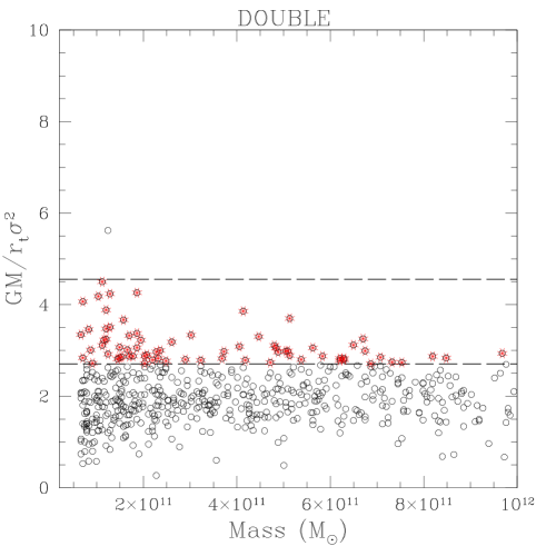
Figure 9: Measured values of $GM_{0}/r_{t}\sigma_{v}^{2}$ versus Mass for the region of the DOUBLE cluster. Groups marked with a star lie within the allowed region where solutions of eq. 13 exist, and the corresponding value of $\zeta_{t}\,$can be found.

Finally, in Figs. 10-11 we plot the $\sigma_{v}-M_{0}$  relation of those halos for which a $\zeta_{t}\,$  can be found, for the DOUBLE and VOID regions, respectively. Note that for these halos the intrinsic dispersion is even smaller than in Figs. 3 and 4. These halos can be then regarded as very near to a TIS equilibrium state. Note also that the coefficient of eq. 1 for the TIS solution has been computed for the minimum energy TIS solution. In fact, from eq. (98) of Shapiro et al. (1999) we see that this coefficient would depend on $\zeta$:

$$\sigma_{v}^{2}=\frac{\left(3\pi G\right)}{5}^{2/3}\frac{\alpha(\zeta)}{\alpha(\zeta)-2}H_{0}^{2/3}(1+z_{coll})M_{0}^{2/3}$$ (14)

where: $\alpha(\zeta)=3\tilde{M}(\zeta)/\zeta^{3}\tilde{\rho}(\zeta)$. As we can see from the figures, the scatter induced by this dependence is very small and less than the intrinsic Poisson scatter.

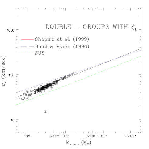
Figure 10: The $\sigma_{v}-M_{0}$  relation for groups in the DOUBLE region for which the truncation radius can be computed by inverting eq. 13. The scatter is less than in the analogous plot for all the groups found by SKID  in the DOUBLE region, Fig. 3. The error bar in the lower left part of the plot represents the uncertainty in the zero point of the best-fit curve induced by the scatter in observed values of $\zeta_{t}$. Notice that it is less than the observed scatter.

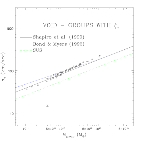
Figure 11: Same as Fig. 10 for the VOID region. Note that the scale of the axes is the same as in Figure 5.

4.3 Probability distribution of the spin parameter

The angular momentum distribution is an interesting statitistics, because the halo angular momentum originates from gravitational interactions between the collapsing region and its environment. Following Peebles (1971) and Efstathiou & Jones (1979) we will present results for the distribution of the spin parameter $\lambda$ defined as:

$$\lambda=\frac{L|E|^{1/2}}{GM^{5/2}}$$ (15)

where $L$ and $|E|$ are the angular momentum and the total energy of each halo, respectively. The calculation of $|E|$ is not free of ambiguities, because in order to compute the potential energy $W$ one should take into account the fact that the halo is not isolated, i.e. one should also account for the contribution from the environmental gravitational field, and this is not currently done by any of the group finders we have adopted. For this reason, we show in Figure 12 the spin probability distribution ${\rm P}(\lambda)$  computed only for TIS halos in the three regions, i.e. for those halos verifying eq. 13. As we have seen in the preceding paragraphs, these halos seem to verify the $\sigma_{v}-M_{0}$  relationship with a much smaller scatter than halos selected by any group finder, so we regard them as our fiducial equilibrium halos. Combining eqs. 44 and 45 from Shapiro et al. (1999) we find that for a TIS halo the total energy $E$ is connected to the potential $W$ by:

$$E=-\frac{2-\alpha}{2(\alpha-1)}W$$ (16)

The potential $W$ for these halos is then computed exactly, i.e. by summing the contribution from each particle in the simulation. Note that the parameter $\alpha$ depends on the dimensionless truncation radius $\zeta_{t}\,$  which can be evaluated only for TIS halos.
One immediately notices that ${\rm P}(\lambda)$  seems to depend on the environment. It has been shown in recent work that a very good fit to ${\rm P}(\lambda)$  is given by a lognormal distribution (Dalcanton et al. 1997; Mo et al. 1998):

$$\lambda{\rm P}(\lambda)=\frac{1}{\sqrt{2\pi}\sigma_{\lambda}}\exp\left\{-\frac{\ln^{2}(\lambda/\langle\lambda\rangle}{2\sigma_{\lambda}^{2}}\right\}d\lambda$$ (17)

Mo et al. (1998) suggest that Eq. 17 with $\langle\lambda\rangle=0.05,\sigma_{\lambda}=0.05$ provides a good fit to the probability distribution of all halos, independently of the environment. What we observe is, on the other hand, that all the three observed distributions seem to be reasonably well fitted by eq. 17, but the values of the fitting parameters are certainly very different from those mentioned above. Moreover, for those halos selected with AFOF, the distributions seem to be all consistent with each other but not well fitted by the lognormal model (Figure 13).
This discrepancy may appear puzzling. However, Figures 12 and 13 cannot be compared, because of two reasons. First, the total energy $E$ entering the definition of $\lambda$ was evaluated directly in Figure 12, while it was estimated from eq. 16 in Figure 8. The procedure we have adopted to extract fiducial TIS halos does actually produce a sample which verifies the $\sigma_{v}-M_{0}$  relationship with a much less statitistical noise than the parent sample. But there is an even stronger reason which makes the comparison doubtful: the total number of halos extracted using AFOF  is much less than that obtained using SKID. Moreover, the extent over $\lambda$ of the spin probability distribution is smaller than for SKID  as is evident from a comparison of the figures. If we take these differences into account, we do not see any significant difference among the distributions in the VOID region. For all these reasons, we can conclude that there is a dependence of the spin probability distribution ${\rm P}(\lambda)$  on the environment only for TIS halos. It would be interesting to speculate about the physical mechanisms producing this dependence, and we hope to be able to address this question in further work.

Table 3: Fits of ${\rm P}(\lambda)$  with lognormal distribution, for TIS halos.

Region	Median	$\langle\lambda\rangle$	$\sigma_{\lambda}$
VOID	0.018	0.018	0.5
DOUBLE	0.018	0.03	0.9
SINGLE	0.051	0.07	1.4
All (SKID)	0.06	0.07	0.65

Before closing this section, we would like to remind the reader that recent theoretical calculations predict a rather large distribution in the average values and shape of ${\rm P}(\lambda)$  , with a rather marked dependence on the peak’s overdensity (Catelan & Theuns 1996) or on the details of the merging histories (Nagashima & Gouda 1998; Vitvitska et al. 2001). A direct comparison of our results with the conditional probability distribution ${\rm P}(\lambda|\nu)$ of Catelan & Theuns (1996) is made difficult by the fact that the relationship between the linear overdensity $\nu$ and (for instance) the final mass of the halo turns out to be quite noisy (Sugerman et al. 2000, Fig. 10), so it is not possible to “label” unambigously each halo with its initial overdensity. However, one could hope to further increase the number of halos by further diminishing the softening length, and we hope to get a better statistics from future simulations which would help us to address also the latter points.

Figure 12: Probability distribution of the spin parameter for the three regions, for TIS halos. The dashed curves are the best-fit approximations obtained using the lognormal distribution adopted by Mo et al. (1998) (eq. 15). Histograms and fitting curves are normalized to unity.

Figure 13: Same as Figure 14 but for halos selected using AFOF. The dashed curve is a lognormal distribution with $\rangle\lambda\langle=0.5,\sigma_{v}=0.05$.

4.4 Density profiles of massive halos

As we already mentioned in the Introduction, even the most massive halos we find in this simulation using SKID  do not contain enough particles to allow a reliable determination of the density profile. This is clearly visible from Figure 13, where we plot the profiles of the four most massive halos extracted from the DOUBLE cluster region. None of these halos lies in the integrability strip of Figure 11, so the best fit TIS profiles displayed as continous curves have been obtained by least square fittings, where we have varied $\rho_{0}$ and $r_{0}$.

Figure 14: Density profiles for the four most massive halos within the DOUBLE region. The number of particles contained in each halo is shown. Best fit solutions using the minimum energy TIS solution by Shapiro et al. (1999) are shown.

The distinguishing feature of the TIS density profile, when compared with the universal density profile of Navarro et al. (1996, 1997) is the presence of a central core. Although the minimum energy TIS profiles fit reasonably well the central regions, they fall out too gently at distances larger than a few times the core radius, and in no case we can find a reasonably good overall agreement. It would be hazardous to draw any conclusion from this comparison, in view of the above mentioned poor resolution. However, a reasonable explanation for the sharp decline of the density profiles is tidal stripping, which should be effective at a few times the core radius.

5 Conclusion

The properties of galaxy-sized halos we have considered in this paper seem to be very constraining for halo collapse and equilibrium models. However, none of the equilibrium models considered (neither the minimum energy TIS model) seems to be able to give a comprehensive description of our findings. We would like to summarize now our findings and to point to some controversial issues that they pose.
First of all, the $\sigma_{v}-M_{0}$  statistics seems to be a sensitive tool to discriminate among different halo equilibrium models. This statistics is easy to evaluate, because it relies on global quantities, and it can then be applied to samples of halos. In this context, it is more difficult to discriminate models using statistics like the density profile, which would require a considerably larger mass range in order to give reliable results (see for instance Jing & Suto 2000).
Models for the $\sigma_{v}-M_{0}$  statistics based on the NFW density profile seem to be only marginally consistent with simulation data. The rôle of the anisotropy parameter in this context does not seem to be crucial: it is the slope of the radius-mass relationship for these halos which seems to mostly affect the normalisation of the $\sigma_{v}-M_{0}$  .
As we have seen, the TIS model seems to offer a very good quantitative framework to explain the $\sigma_{v}-M_{0}$  statistics, even in the VOID region where the slope of the relationship is very different from that predicted by the minimum energy TIS model of Shapiro et al. The fact that a model based on the hypothesis that halos have a finite extent provides a good description should not come as a surprise. Halos forming in clusters experience a complex tidal field originating from neighbouring halos and from the large scale web in which they are embedded. The tidal radii of the environments within which they lie, although often larger than the mean distance, could limit the extent of halos. A theoretical treatment of the growth of the angular momentum is complicated by the fact that the distribution of the torques induced by nearby halos depends on clustering (Antonuccio-Delogu & Atrio-Barandela 1992). However, we believe that it would be difficult to think that the truncation is a numerical artifact due to the finite mass resolution: were this the case, we should expect the same relationship between truncation radius $r_{t}$ and mass in all the three regions, but this is clearly not the case.
We have already noted the fact that the truncation radii we find are always less than the critical value for the onset of gravothermal instability, $\zeta_{crit}=34.2$. This leads us to think that this instability is at work in our simulations, but in order to investigate this issue one would need simulations with a dynamical range at least 3 orders of magnitudes larger than those used in this simulation.
Concerning the dependence of the distribution of spin parameters on the environment, we find that halos selected using AFOF  do not show any dependence on the environment (the same holds for halos selected using SKID ), but if we select subsamples of fiducial TIS halos, we do find a dependence of the properties of ${\rm P}(\lambda)$  on the environment. In particular, this fact seems to be at odds with the recent investigation by Syer et al. (1999), who find that the observed distribution of the spin parameter for a large homogeneous sample of spirals is well described by a lognormal distribution with $\langle\lambda\rangle\approx 0.05$ and a variance $\sigma_{\lambda}\approx 0.36$. This result is in contrast also with other work mentioned above (Warren et al. 1992; Eisenstein & Loeb 1995). If confirmed by further investigations, this discrepancy could suggest that there is probably some systematic trend in the way the angular momentum of the luminous discs is connected with that of the halo, which is not accounted for by the models of Syer et al. (1999).
Last but not least, it is important to stress that Lemson & Kauffmann (1999) conclude that “Only the mass distribution varies as a function of environment. This variation is well described by a simple analytic formula based on the conditional Press–Schechter theory. We find no significant dependence of any other halo property on environment…”. In comparing their results with ours, we must keep in mind that we have followed a very different procedure from theirs, because we have prepared a simulation using constrained initial conditions with the purpose of obtaining a final configuration containing certain features (i.e. a double cluster and a void). Although our simulation box is not an “average” region of the Universe, it is certainly a representative one. We stress again the fact that all the halos from underdense regions in our simulation come from a void, and not from the outer parts of clusters. Lemson & Kauffmann, on the other hand, seem to take their halos from all the volume and group them according to the overdensity of their parent regions. We think then that a direct comparison between the results of these two different investigations would be misleading, given the complementarity of our approaches.

6 Appendix

We give a full derivation of equation 13. The starting point is the virial theorem for systems with boundary pressure terms, as given in eq. 41 from Shapiro et al. (1999):

$$0=2K+W+S_{p}$$ (18)

In the above equation the kinetic energy $K$ can be rewritten in terms of the 1-D velocity dispersion:

$$K=\frac{M_{0}\langle v\rangle^{2}}{2}=\frac{3}{2}M_{0}\sigma_{v}^{2}$$ (19)

The potential energy term $W$:

$$W=4\pi G\int_{0}^{\infty}\rho M(r)rdr\equiv 4\pi G\int_{0}^{r_{t}}\rho M(r)rdr$$ (20)

can be rewritten in terms of global quantities and of the dimensionless radius $\zeta_{t}\,$:

$$W=-\frac{GM_{0}^{2}}{r_{t}}\frac{\zeta_{t}\Psi(\zeta_{t})}{M^{2}(\zeta_{t})}$$ (21)

where we have defined:

$$\Psi(\zeta_{t})=\int_{0}^{\zeta_{t}}d\zeta\zeta\tilde{\rho}(\zeta)\tilde{M}(\zeta)$$

Finally, $S_{p}$ is a surface term which arises from the constraint that the system has a finite radius, and is given by (Shapiro et al., eq. 43):

$$S_{p}=-4\pi r_{0}^{3}p_{t}\zeta_{t}$$ (22)

We are adopting here the same notation as Shapiro et al., so that $r_{0}$ and $p_{t}$ are the core radius and an external “pressure” term, respectively. Using eqs. 34 and 38 from Shapiro et al., the latter equation can be rewritten in terms of the dimensionless integrated mass and density:

$$S_{p}=-\frac{M_{0}}{\tilde{M}_{t}(\zeta_{t})}\tilde{\rho}(\zeta_{t})\sigma_{v}^{2}$$ (23)

Substituting eqs. 19, 21, 23 into eq. 18 we get:

$$3M_{0}\sigma_{v}^{2}=-\frac{GM_{0}^{2}}{r_{t}}\frac{\zeta_{t}\Psi(\zeta_{t})}{M^{2}(\zeta_{t})}-\frac{M_{0}}{\tilde{M}_{t}(\zeta_{t})}\tilde{\rho}(\zeta_{t})\sigma_{v}^{2}$$ (24)

from which we get the desired equation.

References

- Antonov (1962) Antonov, V. A. 1962, ”Solution of the problem of stability of stellar system Emden’s density law and the spherical distribution of velocities” (Vestnik Leningradskogo Universiteta, Leningrad: University, 1962)
- Antonuccio-Delogu & Atrio-Barandela (1992) Antonuccio-Delogu, V. & Atrio-Barandela, F. 1992, ApJ, 392, 403
- Barnes (1987) Barnes, J. 1987, Computer Physics Communications, 87, 161
- Barnes & Hut (1986) Barnes, J. & Hut, P. 1986, Nature, 324, 446
- Becciani et al. (1997) Becciani, U., Ansaloni, R., Antonuccio-Delogu, V., Erbacci, G., Gambera, M., & Pagliaro, A. 1997, Computer Physics Communications, 106, 105
- Becciani et al. (2000) Becciani, U., Antonuccio-Delogu, V., & Gambera, M. 2000, Journal of Computational Physics, 163, 118
- Becciani et al. (1998) Becciani, U., Antonuccio-Delogu, V., Gambera, M., Pagliaro, A., Ansaloni, R., & Erbacci, G. 1998, in ASP Conf. Ser. 145: Astronomical Data Analysis Software and Systems VII, Vol. 7, 7
- Bertschinger (1985) Bertschinger, E. 1985, ApJS, 58, 39
- Binney & Tremaine (1987) Binney, J. & Tremaine, S. 1987, ”Galactic dynamics” (Princeton, NJ, Princeton University Press, 1987)
- Bond & Myers (1996a) Bond, J. R. & Myers, S. T. 1996a, ApJS, 103, 1
- Bond & Myers (1996b) —. 1996b, ApJS, 103, 41
- Bryan & Norman (1998) Bryan, G. L. & Norman, M. L. 1998, ApJ, 495, 80
- Buchert et al. (1999) Buchert, T., Kerscher, M., & Sicka, C. 1999, astro-ph/9912347
- Bullock et al. (2001) Bullock, J. S., Kolatt, T. S., Sigad, Y., Somerville, R. S., Kravtsov, A. V., Klypin, A. A., Primack, J. R., & Dekel, A. 2001, MNRAS, 321, 559
- Catelan & Theuns (1996) Catelan, P. & Theuns, T. 1996, MNRAS, 282, 436
- Couchman (1991) Couchman, H. M. P. 1991, ApJ Letters, 368, L23
- Dalcanton et al. (1997) Dalcanton, J. J., Spergel, D. N., & Summers, F. J. 1997, ApJ, 482, 659+
- Efstathiou & Jones (1979) Efstathiou, G. & Jones, B. J. T. 1979, MNRAS, 186, 133
- Eisenstein & Hut (1998) Eisenstein, D. J. & Hut, P. 1998, ApJ, 498, 137+
- Eisenstein & Loeb (1995) Eisenstein, D. J. & Loeb, A. 1995, ApJ, 439, 520
- Gardner (2000) Gardner, J. 2000, astro-ph/0006342
- Governato et al. (1997) Governato, F., Moore, B., Cen, R., Stadel, J., Lake, G., & Quinn, T. 1997, New Astronomy, 2, 91
- Gunn (1977) Gunn, J. E. 1977, ApJ, 218, 592
- Gunn & Gott (1972) Gunn, J. E. & Gott, J. R. I. 1972, ApJ, 176, 1
- Hernquist et al. (1991) Hernquist, L., Bouchet, F. R., & Suto, Y. 1991, ApJS, 75, 231
- Hoffman & Ribak (1991) Hoffman, Y. & Ribak, E. 1991, ApJ Letters, 380, L5
- Jing & Suto (2000) Jing, Y. P. & Suto, Y. 2000, ApJ Letters, 529, L69
- Knebe & Müller (1999) Knebe, A. & Müller, V. 1999, A& A, 341, 1
- Lemson & Kauffmann (1999) Lemson, G. & Kauffmann, G. 1999, MNRAS, 302, 111
- Łokas & Mamon (2001) Łokas, E. L. & Mamon, G. A. 2001, MNRAS, 321, 155
- Lynden-Bell & Wood (1968) Lynden-Bell, D. & Wood, R. 1968, MNRAS, 138, 495
- Mo et al. (1998) Mo, H. J., Mao, S., & White, S. D. M. 1998, MNRAS, 295, 319
- Moore et al. (1999) Moore, B., Ghigna, S., Governato, F., Lake, G., Quinn, T., Stadel, J., & Tozzi, P. 1999, ApJ Letters, 524, L19
- Nagashima & Gouda (1998) Nagashima, M. & Gouda, N. 1998, MNRAS, 301, 849
- Navarro et al. (1996) Navarro, J. F., Frenk, C. S., & White, S. D. M. 1996, ApJ, 462, 563
- Navarro et al. (1997) —. 1997, ApJ, 490, 493
- Padmanabhan (1993) Padmanabhan, T. 1993, ”Structure formation in the universe” (Cambridge, UK: Cambridge University Press, —c1993)
- Peebles (1971) Peebles, P. J. E. 1971, A& A, 11, 377
- Shapiro et al. (1999) Shapiro, P. R., Iliev, I. T., & Raga, A. C. 1999, MNRAS, 307, 203
- Sugerman et al. (2000) Sugerman, B., Summers, F. J., & Kamionkowski, M. 2000, MNRAS, 311, 762
- Syer et al. (1999) Syer, D., Mao, S., & Mo, H. J. 1999, MNRAS, 305, 357
- Takada & Futamase (1999) Takada, M. & Futamase, T. 1999, General Relativity and Gravitation, 31, 461
- van de Weygaert & Bertschinger (1996) van de Weygaert, R. & Bertschinger, E. 1996, MNRAS, 281, 84
- van Kampen & Katgert (1997) van Kampen, E. & Katgert, P. 1997, MNRAS, 289, 327
- Vitvitska et al. (2001) Vitvitska, M., Klypin, M., Kravtsov, A., Bullock, J., Wechsler, R., & Primack, J. 2001, astro-ph/0105349
- Warren et al. (1992) Warren, M. S., Quinn, P. J., Salmon, J. K., & Zurek, W. H. 1992, ApJ, 399, 405
- White (1996) White, S. D. M. 1996, in Gravitational dynamics, 121
- White (1997) White, S. D. M. 1997, in The Evolution of the Universe: report of the Dahlem Workshop on the Evolution of the Universe, 227
- White & Rees (1978) White, S. D. M. & Rees, M. J. 1978, MNRAS, 183, 341