Construction of Cosmic String Induced Temperature Anisotropy Maps with CMBFAST and Statistical Analysis

Abstract

We use the publicly available code CMBFAST as modified by L. Pogosian and T. Vachaspati to simulate the effects of wiggly cosmic strings on the Cosmic Microwave Background (CMB). Using the modified CMBFAST code which takes into account vector modes and models wiggly cosmic strings by the one scale model, we go beyond the angular power spectrum to construct CMB temperature maps with resolution of a few degrees. The statistics of these maps are then studied using conventional and recently proposed statistical tests optimized for the detection of hidden temperature discontinuities induced by the Gott-Kaiser-Stebbins effect. We show however, that these realistic maps can not be distinguished in a statistically significant way from purely Gaussian maps with identical power spectrum.

I Introduction

A promising method of identifying the origin of the large–scale structure of the universe, is the statistical analysis of the CMB fluctuations [1-5]. What one hopes to get out of this is the possible distinction between the two major classes of physical theories of structure formation, namely theories of inflation [6] and topological defects [7]. An important differentiating feature of these two classes of theories is the statistics of primordial fluctuations. Temperature anisotropies $\frac{\Delta T}{T}$ of the CMB, if originating from quantum fluctuations in an inflationary context, should obey Gaussian statistics. However, the confidence by which the CMB anisotropies were shown to follow that statistic is reduced [8], taking in mind the work done by [9, 10] using COBE–DMR maps. This could favor topological defect theories.

Cosmic strings seeding structure formation [11-15] consist a promising case of these theories. However, despite the significant progress made recently [12,13,16-18] in understanding the effects of cosmic strings on the CMB, the uncertainty of the derived predictions remains significant [19, 20]. The main source of this uncertainty is that there is no simple way to characterize the network of strings. In order to bypass this difficulty various studies have attempted to model the string network by incorporating simplifying assumptions. Such simplifications have made possible the realization of cosmological string network simulations [21-23] that attempt to model evolution in a very wide range of scales. They have also made possible the construction of semi-analytical models that attempt to capture features missed by the inherent limitations of full scale numerical simulations. For example, early work [24, 25] based on the latter approach had revealed important features of the cosmic string induced CMB fluctuations that were missed by detailed numerical simulations. In particular it was shown[25], using a simple model of string network evolution, that the wiggles (small scale structure) of long cosmic strings tend to amplify the height of the Doppler peak of the CMB angular spectrum of string induced fluctuations.

The main reason for this amplification may be attributed to the two main factors that determine the string induced fluctuations. These are, first the Integrated Sachs–Wolfe effect (long strings present between last scattering and the present time interacting gravitationally directly with the photons) for scales larger than 2 degrees and second, for scales about 1-2 degrees, interactions of the photons with the string perturbed plasma performing acoustic oscillations on the last scattering surface (LSS) excited by long strings. It may be shown [25-27] that the latter effect leads to temperature fluctuations ${\Delta T}\over T$ that are amplified compared to the fluctuations induced by the former effect. The amplification factor $\lambda>1$ is due to the fact that the wiggles do not interact gravitationally directly with the photons, while they do interact with the plasma [25, 27] on the LSS leading indirectly to additional fluctuations on the CMB through the last scattering of photons on the fast moving plasma electrons. Therefore this amplification can only affect the last scattering horizon scale, i.e. a scale of about 1-2 degrees. The factor $\lambda$ can be expressed as [25, 27]

$$\lambda=(1+{{(1-{T\over\mu})}\over{2<(v_{s}\gamma_{s})^{2}>}})$$ (1)

where T is the tension of the wiggly long string which decreases with the wiggliness and is estimated by simulations to be $T\simeq 0.7\mu$ where $\mu$ is the mass per unit length of the string. Also, $v_{s}$ is the string velocity and $\gamma_{s}$ the corresponding Lorentz factor.

This result of Doppler peak amplification due to cosmic string wiggles has recently been verified by the numerical modeling developed by Pogosian and Vachaspati [26]. These authors used the line of sight integration approach of the publicly available code CMBFAST [28] combined with the one–scale model [29, 30] for wiggly cosmic string evolution to derive the angular CMB power spectrum and the matter power spectrum. One of their main results was that small scale structure (wiggles) of long strings tends to increase the height of the Doppler peak of the CMB spectrum thus confirming the expectations of Ref. [25] and improving the agreement of the predicted angular spectrum with observations.

In the present work we use the approach of Pogosian and Vachaspati and modify their publicly available code based on CMBFAST to go beyond the CMB spectrum and construct realistic maps of CMB fluctuations produced by wiggly strings. Our goal is to apply statistical tests on several realizations of these maps and attempt to identify their non-Gaussian features. Some of the tests we applied [31] (which were specially designed for this purpose) were able to identify non-Gaussian features on simple CMB maps [9], constructed by the superposition of a small temperature discontinuity (produced by a single long string via the Gott-Kaiser-Stebbins effect [32, 33]) on a Gaussian background. In the present study however, we show that these same tests are not able to identify the string induced non-Gaussianity of more realistic maps on the scales considered. This is due to the fact that the superposition of several line-like temperature discontinuities tends to wash out the effects of each individual discontinuity and reduces the effectiveness of the proposed tests. Therefore, the detection of the small non-Gaussianity induced by cosmic strings on a few degrees scale remains a challenging open issue.

II Construction of the maps

The construction of the CMB temperature anisotropy maps on which the statistical tests were performed, was made possible by two major contributions: the wiggly string  one–scale model as the cosmic string network model and the use of the line of sight integration approach.

The cosmic string network model that we used is the one found in detail in [26]. Briefly, the network is approximated [12-14] by a collection of uncorrelated straight string segments which are assumed to be produced at some early epoch, with positions drawn randomly from a uniform distribution in space, moving with random uncorrelated velocities, their directions drawn from a uniform distribution on a two sphere. This model has the merit of being relatively simple and amenable to modifications that seem to be indicated by direct simulations [23, 34].

Small–scale structure, wiggles, were incorporated in order to make the model more realistic, since lattice simulations of string formation and evolution [23] suggest that strings are not straight. However, a distant observer would not be able to discern this small–scale structure, but see instead a smooth string with effective mass per unit length $\tilde{U}$ and tension $\tilde{T}$. The wiggly string is heavier and slower than the ordinary Nambu-Goto straight string (whose equation of state is: $\mu_{0}=T$, where $\mu_{0}$ is the mass per unit length). The equation of state of a wiggly string (averaged over the small–scale structure) is [35, 36]:

$$\tilde{U}\tilde{T}=\mu_{0}^{2},$$ (2)

$$\tilde{U}=\alpha\mu_{0},\ \tilde{T}=\mu_{0}/\alpha$$ (3)

where $\alpha$ is the “wiggliness” parameter, estimated [23] in the radiation and matter eras to be $\alpha_{r}\simeq 1.9$ and $\alpha_{m}\simeq 1.5$ respectively. The expected evolution of the wiggliness parameter is fitted by [23, 26]:

$$\alpha(\tau)=1+\frac{(\alpha_{r}-1)a}{\tau\dot{a}}$$ (4)

where $a$ is the scale factor.

The parameters of the segments: length, velocity and wiggliness are modeled using the  one–scale model [29, 30]. The evolution of the two competing processes of string stretching on the one hand (due to cosmic expansion), and the chopping off of loops and their subsequent decay on the other (due to long string reconnection), are described by [37]:

$$\frac{dl}{d\tau}=\frac{\dot{a}}{a}lv^{2}+\frac{1}{2}\tilde{c}v$$ (5)

$$\frac{dv}{d\tau}=(1-v^{2})(\frac{\tilde{k}}{l}-2\frac{\dot{a}}{a}v)$$ (6)

where $l$ is the comoving correlation length, $v$ is the $rms$ string velocity, $\tilde{c}$ is the loop chopping efficiency and $\tilde{k}$ is the effective curvature of the strings [13]. At every subsequent epoch, a certain fraction of the number of segments decays in a way that preserves scaling.

The Fourier transform of the energy–momentum tensor for an individual string segment $m$ is:

$$\Theta_{00}^{m}=\frac{\mu\alpha}{\sqrt{1-v^{2}}}\frac{\sin{(k\hat{X}^{\prime}_{3}l/2)}}{k\hat{X}^{\prime}_{3}l/2}\cos{({\bf{k}}\cdot{\bf{x_{0}}}+k\hat{\dot{X}}_{3}v\tau),}$$ (7)

$$\Theta_{ij}^{m}=\left[v^{2}\hat{\dot{X}}_{i}\hat{\dot{X}_{j}}-\frac{(1-v^{2})}{\alpha^{2}}\hat{X^{\prime}}_{i}\hat{X^{\prime}}_{j}\right]\Theta_{00},$$ (8)

while $\Theta_{0i}^{m}$ can be found from the relation: $\nabla^{\mu}\Theta_{\mu\nu}^{m}=0$. ($X^{\mu}(\sigma,\tau)$ are the coordinates of the segments: $X^{0}=\tau,\hskip 5.69054pt{\bf{X}}={\bf{x}_{0}}+\sigma\hat{{\bf{X^{\prime}}}}+v\tau\hat{{\bf{\dot{X}}}}$, where ${\bf{x}_{0}}$ is the random location of the center of mass, $\hat{{\bf{X^{\prime}}}}$ and $\hat{{\bf{\dot{X}}}}$ are unit vectors along and perpendicular to the string which are randomly oriented, also satisfying $\hat{{\bf{X}^{\prime}}}\cdot\hat{{\bf{\dot{X}}}}=0$ and $\sigma$ is the coordinate along the string).

A consolidation of all string segments that decay at the same epoch into one with the appropriate statistical weight is used, as was suggested in [12], so that the number of segments can be dealt with computationally. The total energy–momentum tensor of the network is the sum over the contributions of the consolidated string segments [26]:

$$\Theta_{\mu\nu}({\bf{k}},\tau)=\sum^{N_{0}}_{m=1}\Theta_{\mu\nu}^{m}({\bf{k}},\tau)T^{off}(\tau,\tau_{m}),$$ (9)

where $N_{0}$ is the initial number of segments, and $T^{off}$ is a smooth function that turns off the $m^{th}$ segment by time $\tau_{m}$ [12, 13]. $\Theta_{\mu\nu}({\bf{k}},\tau)$ will be incorporated into the sources: $S(k,\tau)$ (cf eqs.(14,16)).

Our main goal is to compute the CMB anisotropy seeded by cosmic strings:

$$\frac{\Delta T}{T}(\hat{{\bf{n}}})\equiv\frac{\Delta T}{T}({\bf{x}}=0,\hat{{\bf{n}}},\tau_{0})=\sum_{l,m}a_{lm}Y_{lm}(\hat{{\bf{n}}})$$ (10)

(${\bf{x}}$ is the position of the observer and $\hat{{\bf{n}}}$ is the line of sight direction). The code of [26] (based on CMBFAST ) which we modified and used, uses the line of sight integration approach [28] to compute, among other things, the angular power spectrum $C_{l}$:

$$C_{l}=\frac{1}{2l+1}\sum^{l}_{m=-l}<a_{lm}^{*}a_{lm}>$$ (11)

originating from temperature perturbations seeded by cosmic strings by incorporating the sources into $\Theta_{\mu\nu}$ in the way described below.

The Fourier transform $\Delta({\bf{k}},\hat{{\bf{n}}},\tau_{0})$ of $\frac{\Delta T}{T}(\hat{{\bf{n}}})$ depends only on the angle $q$ between the two vectors $(q\equiv\hat{{\bf{k}}}\cdot\hat{{\bf{n}}})$ and can be expanded in multipole moments $\Delta_{l}({\bf{k}},\tau_{0})$ [38]:

$$\Delta({\bf{k}},\hat{{\bf{n}}},\tau_{0})=\sum^{\infty}_{l=0}(-i)^{l}(2l+1)\Delta_{l}({\bf{k}},\tau_{0})P_{l}(\hat{{\bf{k}}}\cdot\hat{{\bf{n}}})$$ (12)

further, $\Delta_{l}({\bf{k}},\tau_{0})$ is decomposed into [38]:

$$\Delta_{l}({\bf{k}},\tau_{0})\equiv\xi({\bf{k}})\Delta_{l}(k,\tau_{0})$$ (13)

However, according to the line of sight integration approach [28, 39]:

$$\Delta(k,q,\tau_{0})=\int_{0}^{\tau_{0}}e^{ikq(\tau-\tau_{0})}S(k,\tau)d\tau$$ (14)

where the term $S(k,\tau)$ contains the contributions from all the sources, as well as $\Theta_{\mu\nu}$ from the string network [28]. Using the relation:

$$e^{ikq(\tau-\tau_{0})}=\sum_{l}(-i)^{l}(2l+1)j_{l}[k(\tau_{0}-\tau)]P_{l}(q)$$ (15)

we get [28]:

$$\Delta_{l}(k,\tau_{0})=\int_{0}^{\tau_{0}}S(k,\tau)j_{l}[k(\tau_{0}-\tau)]d\tau$$ (16)

In order to get the $a_{lm}$ coefficients needed to construct the maps, we have to assume arbitrary direction for $\hat{{\bf{k}}}$, or equivalently use the more general relation :

$$e^{i{\bf{k}}\cdot{\bf{r}}}=4\pi\sum_{l=0}^{\infty}\sum_{m=-l}^{l}i^{l}j_{l}(kr)Y^{*}_{lm}(\hat{{\bf{k}}})Y_{lm}(\hat{{\bf{r}}})$$ (17)

in (12,14). Otherwise we would be able to compute only the $a_{l0}$ terms as we shall see next. Then (16) still holds. The $a_{lm}$s read [38]:

$$a_{lm} = \int d\Omega Y^{*}_{lm}(\hat{{\bf{n}}})\frac{\Delta T}{T}(\hat{{\bf{n}}})=4\pi(-i)^{l}\int d^{3}{\bf{k}}Y^{*}_{lm}(\hat{{\bf{k}}})\Delta_{l}({\bf{k}},\tau_{0})$$ (18)

$$= 4\pi(-i)^{l}\int d^{3}{\bf{k}}Y^{*}_{lm}(\hat{{\bf{k}}})\xi({\bf{k}})\Delta_{l}(k,\tau_{0})$$ (19)

where $\Delta_{l}(k,\tau_{0})$ is given in (16) (had we not assumed the arbitrariness of $\hat{{\bf{k}}}$, we would only get: $a_{lm}=(-i)^{l}\sqrt{4\pi(2l+1)}\int d^{3}{\bf{k}}\xi({\bf{k}})\Delta_{l}(k,\tau_{0})\delta_{m0}=a_{l0})$.

Since the linearized Einstein equations may be decomposed into scalar, vector and tensor parts (S, V, T) [40], we have three distinct contributions to the sources (e.g. S: density perturbations, V: cosmic strings, T: gravitational radiation, [13, 16]). So, $(\Delta,\Delta_{l})$ are actually: $(\Delta^{I},\Delta^{I}_{l})$, where $I\equiv S,V,T$. Then:

$$a_{lm}=a^{S}_{lm}+a^{V}_{lm}+a^{T}_{lm},$$ (20)

while $C_{l}=C^{S}_{l}+C^{V}_{l}+C^{T}_{l}$. Following the normalization used in the code, the $a_{lm}$s are defined as:

$$a^{S}_{lm}=\sqrt{\frac{4}{\pi}}\int d^{3}{\bf{k}}Y^{*}_{lm}(\hat{{\bf{k}}})\Delta^{S}_{l}({\bf{k}},\tau_{0})$$ (21)

$$a^{V}_{lm}=\sqrt{\frac{4}{\pi}l(l+1)}\int d^{3}{\bf{k}}Y^{*}_{lm}(\hat{{\bf{k}}})\Delta^{V}_{l}({\bf{k}},\tau_{0})$$ (22)

$$a^{T}_{lm}=\sqrt{\frac{4}{\pi}\frac{(l+2)!}{(l-2)!}}\int d^{3}{\bf{k}}Y^{*}_{lm}(\hat{{\bf{k}}})\Delta^{T}_{l}({\bf{k}},\tau_{0})$$ (23)

where: $\Delta^{I}_{l}({\bf{k}},\tau_{0})\equiv\xi({\bf{k}})\Delta^{I}_{l}(k,\tau_{0})$. In order to implement this scheme, we had to extend the code of [26] to provide for the amplitude of the initial perturbations $\xi({\bf{k}})$, which must be such that [38, 39, 41]:

$$<\xi^{*}({\bf{k}})\ \xi({\bf{k^{\prime}}})>=P_{\xi}(k)\ \delta({\bf{k}}-{\bf{k^{\prime}}})$$ (24)

where $P_{\xi}(k)$ is their power spectrum.

As in [26], we chose the initial power spectrum to be that of white–noise, i.e. $P_{\xi}(k)=$ constant. Consequently, $\xi({\bf{k}})$ was chosen to be proportional to a uniformly random number: $\xi_{{\bf{k}}}\ \epsilon[-1,1]$. Since: $<\xi_{{\bf{k}}}\xi_{{\bf{k^{\prime}}}}>=\frac{1}{3}\delta_{{\bf{kk^{\prime}}}}$, each $a^{I}_{lm}$ was multiplied by a factor of $\sqrt{3}$ when the ensemble average $<a^{I*}_{lm}a^{I}_{lm}>$ was taken in order to compute and verify the $C^{I}_{l}$s .

Applying: $\int d^{3}{\bf{k^{\prime}}}<\xi^{*}({\bf{k}})\ \xi({\bf{k^{\prime}}})>=P_{\xi}(k)$ to our discrete case we get: $\sum_{{\bf{k}}}\Delta V_{{\bf{k}}}<\xi_{{\bf{k}}}\xi_{{\bf{k^{\prime}}}}>=\frac{1}{3}\sum_{{\bf{k}}}\Delta V_{{\bf{k}}}\delta_{{\bf{kk^{\prime}}}}=\frac{1}{3}\Delta V_{{\bf{k}}}$. This leads to the definition of $\xi({\bf{k}})$ as:

$$\xi({\bf{k}})\equiv\frac{\xi_{{\bf{k}}}}{\sqrt{\Delta V_{{\bf{k}}}}},\hskip 11.38109pt\xi_{{\bf{k}}}:random\ \epsilon[-1,1]\ ,$$ (25)

$$\Delta V_{{\bf{k}}}\equiv k^{2}dk\ d\Omega(\hat{{\bf{k}}})$$ (26)

Having chosen this particular realization for $\xi({\bf{k}})$, we can proceed to the construction of the temperature anisotropy maps using eqs.(10,21).

III Results

We chose to construct maps with $l=40$, so that the pixel size is comparable to that of the COBE maps, although our method enables us to proceed even up to much higher $l$s (e.g. $l\simeq 1500$), with greater cost in computational time though. The angular power spectrum of such a map is depicted in Fig.1 in agreement with Ref. [26].

FIG. 1.: Angular power spectrum of a $l=1500$ map.

A typical example of such a map is depicted in Fig.2, where a $30^{\circ}\times 30^{\circ}$ patch of a standardized temperature anisotropy map is shown.

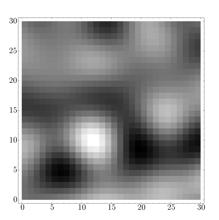
FIG. 2.: A $30^{\circ}\times 30^{\circ}$ patch of one of the constructed standardized temperature anisotropy maps. (Lighter colors correspond to higher values of $\frac{\Delta T}{T}$).

We have applied statistical tests on the above maps in an attempt to identify possible non-Gaussian features. Such statistical tests [31] have recently been proposed for the detection of the particular type of non–Gaussianity induced by coherent discontinuities (edges) hidden in CMB maps. The main advantage of these statistical tests is that they focus on the large–scale coherent properties of CMB maps and are therefore effective even in cases of low resolution maps provided that the area covered is large. The statistics calculated for maps of CMB anisotropies seeded by cosmic strings which we have constructed are the skewness, kurtosis and the recently devised MSD, SMD [31] which are optimized for the detection of coherent discontinuities in 1-D and 2-D pixel maps. It should be pointed out that the skewness and kurtosis statistics have proven[31] to be notably unsuitable to detect the subtle non-Gaussianity in CMB maps. However they have been used as a benchmark[31] to test the effectiveness of more complex statistics like the SMD and the MSD specially designed for the detection of specific types of non-gaussian signatures.

In addition to the statistics discussed here, there are a number of other more complex statistics[42] (minkowski functionals and bispectrum and higher order cumulant estimates in harmonic space) that may be applied to CMB maps to check for non-Gaussianity or topological signatures of defects. Those statistics which are particularly effective on high resolution CMB maps have been discussed extensively in the literature and their application on string maps produced by CMBFAST can be an interesting extension of the present work. Here we focus on the MSD and SMD statistics which are specially designed[9] to detect the specific signature of large scale coherent discontinuities on CMB maps of low resolution.

Assuming a $30^{\circ}\times 30^{\circ}$ (in pixels) standardized temperature map $T_{ij}$($i,j=1,\ldots,30$), the skewness $s$ and kurtosis $k$ are defined as :

$$s=<T^{3}>\equiv\sum_{i,j}T_{ij}^{3}/(30)^{2},$$ (27)

$$k=<T^{4}>\equiv\sum_{i,j}T_{ij}^{4}/(30)^{2}.$$ (28)

These are conventional statistics and their values for Gaussian maps with uncorrelated pixels are $s=0,k=3$. To define the statistics MSD and SMD we consider a partition of the CMB maps in two parts separated by a random curve. In this study we have considered straight lines as well as right angles. Let $\bar{k}$ denote the set of parameters that define the partition line and let $\bar{T_{u}}$ and $\bar{T_{l}}$ be the mean temperatures of the two parts of the map (the indices “u” and “l” stand for “upper” and “lower” parts). The statistical variable $Y_{\bar{k}}$ is defined as :

$$Y_{\bar{k}}\equiv|\bar{T_{u}}-\bar{T_{l}}|.$$ (29)

The statistics MSD and SMD are defined as:

$$MSD\equiv\frac{1}{N}\sum_{\bar{k}}Y_{\bar{k}},$$ (30)

$$SMD\equiv\max(Y_{\bar{k}}),$$ (31)

where $N$ is the total number of partitions. Both MSD and SMD approach asymptotic values for large-$N$. Consider now a Gaussian pattern of temperature fluctuations with a small coherent temperature discontinuity defined by a partition $\bar{k_{0}}$ superposed on the map with coherence scale comparable to the size of the pattern. In [31] it was shown that the presence of such a discontinuity can be detected much more efficiently by the statistics MSD and SMD than by the skewness and kurtosis. A physically motivated mechanism which can lead to the production of a coherent discontinuity on CMB maps is the presence of a moving long cosmic string in our horizon via the fore-mentioned Gott-Kaiser–Stebbins effect [32, 33].

The four statistical tests (MSD, SMD, skewness, kurtosis) have been performed on patches of the maps (Fig.2) produced by the simulation in a way similar to the one in [9]:

• First the values of the 4 statistical variables were computed for a specific $30^{\circ}\times 30^{\circ}$ patch obtained using the simulation code.

• A large number (1200) of Gaussianized maps were constructed from this patch by randomizing the phases in Fourier space and using a Gaussian spectrum with 0 mean and variance equal to the measured spectrum of the map.

• The 4 statistics were calculated for each of these Gaussianized maps.

• Using these results, the probability distribution for each statistic was constructed.

• Finally, the probability for obtaining the already calculated (in step 1) values of the 4 statistics was found.

The results are shown in Figs. 3, 4. Clearly, the applied statistics can not reveal non-Gaussianity in a statistically significant amount in the maps produced by the simulation. The values of the statistics considered for the string induced maps (black dots) are within $1\sigma$ in the probability distributions produced by the gaussianized maps.

FIG. 3.: Probability distribution of the MSD based on 1200 Gaussianized maps. The probability for obtaining the MSD value of the string–induced map (MSD=7.378, represented by the dot) is 0.35.

FIG. 4.: Probability distribution of the kurtosis based on 1200 Gaussianized maps. The probability for obtaining the kurtosis value of the string–induced map (kurtosis=3.08, represented by the dot) is 0.17.

We have also extended the above results using right angles as partition lines instead of straight lines. However, the sensitivity of the statistics considered was not increased, rendering results similar to Figs. 3, 4.

IV Concluding Remarks

String–induced maps on large angular scales are hard to distinguish from maps with Gaussian fluctuations, even using specially designed tests. We have suggested a technique for constructing string-induced temperature anisotropy maps which can be exploited in many ways. The maps constructed the way described in section 2 are proved not to be dominated by late long strings. On the contrary, small–scale structure features come into play which, in a way, destructively interfere and ruin the large–scale coherence which the MSD and SMD tests are proposed to optimally detect. Thus, we offered a confirmation to the fact that string–induced temperature anisotropy maps are practically Gaussian on large scales.

V Acknowledgements

We would like to thank Levon Pogosian and Tanmay Vachaspati for their assistance in acquiring and better understanding the code they developed by modifying CMBFAST.

REFERENCES

- [1] J. Gott et al., Ap. J 352, 1 (1990).
- [2] R. Moessner, L. Perivolaropoulos, and R. Brandenberger, Ap. J. 425, 365 (1994).
- [3] J. Magueijo, Phys. Rev. D 52, 4361 (1995).
- [4] P. G. Ferreira and J. Magueijo, Phys. Rev. D 56, 4578 (1997).
- [5] A. Lewin, A. Albrecht, and J. Magueijo, Mon. Not. R. Astron. Soc. 302, 131 (1999).
- [6] D. Lyth, Phys. Rept. 314, 1 (1999).
- [7] A. Vilenkin and E. Shellard, in Cosmic Strings and other Topological Defects, edited by P. Landshoff (Cambridge University Press, Cambridge CB2 1RP, 1994).
- [8] A. Kogut et al., Ap. J. Lett. 464, L29 (1996).
- [9] L. Perivolaropoulos and N. Simatos, Mod. Phys. Lett. A 13, 2945 (1998).
- [10] P. G. Ferreira, J. Magueijo, and K. Gorski, Ap. J. 503, L1 (1998).
- [11] U. Pen, U. Seljak, and N. Turok, Phys. Rev. Lett. 79, 1611 (1997).
- [12] A. Albrecht, R. Battye, and J. Robinson, Phys. Rev. Lett. 79, 4736 (1997).
- [13] A. Albrecht, R. Battye, and J. Robinson, Phys. Rev. D 59, 023508 (1999).
- [14] R. Battye, J. Robinson, and A. Albrecht, Phys. Rev. Lett. 80, 4847 (1998).
- [15] C. Contaldi, M. Hindmarsh, and J. Magueijo, Phys. Rev. Lett. 82, 679 (1999).
- [16] N. Turok, U. Pen, and U. Seljak, Phys. Rev. D 58, 023506 (1998).
- [17] U. Seljak, U. Pen, and N. Turok, Phys. Rev. Lett. 79, 1611 (1997).
- [18] U. Seljak, U. Pen, and N. Turok, Phys. Rev. Lett. 79, 1615 (1997).
- [19] A. Riazuelo, N. Deruelle, and P. Peter, astro-ph/9910290 (1999).
- [20] R. Durer and M. Sakelariadou, Phys. Rev. D 56, 4480 (1997).
- [21] B. Allen et al., Phys. Rev. Lett. 79, 2624 (1997).
- [22] B. Allen et al., Phys. Rev. Lett. 77, 3061 (1996).
- [23] D. Bennett and F. Bouchet, Phys. Rev. D 41, 2408 (1990).
- [24] L. Perivolaropoulos, Phys. Lett. B 298, 305 (1993).
- [25] L. Perivolaropoulos, Ap. J. 451, 429 (1995).
- [26] L. Pogosian and T. Vachaspati, Phys. Rev. D 60, 083504 (1999).
- [27] T. Vachaspati and A. Vilenkin, Phys. Rev. Lett. 67, 1057 (1991).
- [28] U. Seljak and M. Zaldarriaga, Ap. J. 469, 437 (1996).
- [29] T. Kibble, Nucl. Phys. B 252, 227 (1985).
- [30] T. Kibble, Nucl. Phys. B 261, 750 (1986).
- [31] L. Perivolaropoulos, Phys. Rev. D 58, 103507 (1998).
- [32] J. Gott, Ap. J. 288, 422 (1985).
- [33] N. Kaiser and A. Stebbins, Nature 310, 391 (1984).
- [34] D. Bennett, F. Bouchet, and A. Stebbins, Nature(London) 335, 410 (1988).
- [35] B. Carter, Phys. Rev. D 41, 3869 (1990).
- [36] A. Vilenkin, Phys. Rev. D 41, 3038 (1990).
- [37] C. Martins and E. Shellard, Phys. Rev. D 54, 2535 (1996).
- [38] C. P. Ma and E. Bertschinger, Ap. J. 455, 7 (1995).
- [39] U. Seljak, Ap. J. 482, 6 (1997).
- [40] R. Crittenden and N. Turok, Phys. Rev. Lett. 75, 2642 (1995).
- [41] M. Zaldarriaga and U. Seljak, Phys. Rev. D 55, 1830 (1997).
-
[42]
J.Magueijo,
Phys.Lett.B 342 32-39 (1995), ERRATUM- ibid. B352 499 (1995)
P.Ferreira and J.Magueijo, Phys.Rev. D 55 3358 (1997)
P. Ferreira, J. Magueijo, and J. Silk, Phys.Rev. D56 , 4592-4603 (1997).