Gravitational Collapse in Turbulent Molecular Clouds. II. Magnetohydrodynamical Turbulence

Abstract

Hydrodynamic supersonic turbulence can only prevent local gravitational collapse if the turbulence is driven on scales smaller than the local Jeans lengths in the densest regions, a very severe requirement (Paper I). Magnetic fields have been suggested to support molecular clouds either magnetostatically or via magnetohydrodynamic (MHD) waves. Whereas the first mechanism would form sheet-like clouds, the second mechanism not only could exert a pressure onto the gas counteracting the gravitational forces, but could lead to a transfer of turbulent kinetic energy down to smaller spatial scales via MHD wave interactions. This turbulent magnetic cascade might provide sufficient energy at small scales to halt local collapse.

We test this hypothesis with MHD simulations at resolutions up to $256^{3}$ zones, done with ZEUS-3D. We first derive a resolution criterion for self-gravitating, magnetized gas: in order to prevent collapse of magnetostatically supported regions due to numerical diffusion, the minimum Jeans length must be resolved by four zones. Resolution of MHD waves increases this requirement to roughly six zones. We then find that magnetic fields cannot prevent local collapse unless they provide magnetostatic support. Weaker magnetic fields do somewhat delay collapse and cause it to occur more uniformly across the supported region in comparison to the hydrodynamical case. However, they still cannot prevent local collapse for much longer than a global free-fall time.

1 Introduction

All star formation takes place in molecular clouds. However, the star formation rate in these clouds is surprisingly low. From the Jeans argument one would expect that they should collapse within their free fall time

$$t_{\rm ff}=\sqrt{\frac{3\pi}{32G\bar{\rho}}}\approx(1.06\times 10^{6}\mbox{ yr})\left(\frac{n}{10^{3}\mbox{ cm}^{-3}}\right)^{-1/2},$$ (1)

where $\bar{\rho}$ is the mean mass density of the cloud, $G$ the gravitational constant and $n=\bar{\rho}/\mu$ the number density, with $\mu=2.36m_{H}$. A catastrophic collapse of a giant molecular cloud on this timescale would yield a single starburst event. However, molecular clouds have classically been thought to survive without global collapse for much longer than their free-fall time $t_{\rm ff}$ (Blitz & Shu 1980). Moreover, stars are not usually observed in nearby star-forming regions to form in such a catastrophic collapse. Instead, they form in localized regions dispersed through an apparently stable cloud.

Observations of spectral line widths in molecular clouds show that the gas moves at speeds exceeding the thermal velocities by up to an order of magnitude (Williams et al. 1999). These supersonic motions seem not to be ordered, so that turbulent support models have often been suggested, with the turbulence giving rise to an effectively isotropic turbulent pressure counteracting the gravitational forces.

However, such models have two problems. First, simulations of supersonic, compressible turbulence show that it typically decays in a time less than the cloud’s free-fall time $t_{\rm ff}$ (Gammie & Ostriker 1996, Mac Low et al. 1998, Mac Low 1999). So, in order to be really able to support the cloud, the turbulence would have to be constantly driven. Second, although hydrodynamical turbulence can prevent global collapse, it can never completely prevent local collapse except with unrealistically short driving length scale $\lambda_{D}$ (Klessen, Heitsch & Mac Low 2000; hereafter Paper I). The efficiency of local collapse depends on the wavelength and on the strength of the driving source. Long wavelength driving or no driving at all results in efficient, coherent star formation, with most collapsed regions forming near each other (Klessen & Burkert 2000). Strong, short wavelength driving, on the other hand, results in inefficient, incoherent star formation, with isolated collapsed regions randomly distributed throughout the cloud.

The model of molecular clouds being supported by turbulence has been widely discussed and investigated, as reviewed in Paper I and Vázquez-Semadeni et al. (2000). Recently, Ballesteros-Paredes et al. (1999), Hennebelle & Pérault (1999), and Elmegreen (2000) have suggested that molecular clouds might not have to be supported for these long time scales at all, but might be transient features caused by colliding flows in the interstellar medium. This would solve very naturally not only the problem of cloud support, but also, according to Ballesteros-Paredes et al. (1999), the pronounced lack of 5–10 million year old post-T Tauri-stars directly associated with star-forming molecular clouds.

Magnetic fields might alter the dynamical state of a molecular cloud sufficiently to prevent gravitationally unstable regions from collapsing (McKee 1999). They have been hypothesized to support molecular clouds either magnetostatically or dynamically through MHD waves.

Mouschovias & Spitzer (1976) derived an expression for the critical mass-to-flux ratio in the center of a cloud for magnetostatic support. Assuming ideal MHD, a self-gravitating cloud of mass $M$ permeated by a uniform flux $\Phi$ is stable if the mass-to-flux ratio

$$\frac{M}{\Phi}<\left(\frac{M}{\Phi}\right)_{cr}\equiv\frac{c_{\Phi}}{\sqrt{G}}.$$ (2)

with $c_{\Phi}$ depending on the geometry and the field and density distribution of the cloud. A cloud is termed subcritical if it is magnetostatically stable and supercritical if it is not. Mouschovias & Spitzer (1976) determined that $c_{\Phi}=0.13$ for their spherical cloud. Assuming a constant mass-to-flux ratio in a region results in $c_{\Phi}=1/(2\pi)\simeq 0.16$ (Nakano & Nakamura 1978). Without any other mechanism of support such as turbulence acting along the field lines, a magnetostatically supported cloud will collapse to a sheet which then will be supported against further collapse. Fiege & Pudritz (1999) discussed a sophisticated version of this magnetostatic support mechanism, in which poloidal and toroidal fields aligned in the right configuration could prevent a cloud filament from fragmenting and collapsing.

Investigation of the second alternative, support by MHD waves, concentrates mostly on the effect of Alfvén waves, as they (1) are not as subject to damping as magnetosonic waves and (2) can exert a force along the mean field, as shown by Dewar (1970) and Shu et al. (1987). This is because Alfvén waves are transverse waves, so they cause perturbations $\delta\mathbf{B}$ perpendicular to the mean magnetic field $\mathbf{B}$. McKee & Zweibel (1994) argue that Alfvén waves can even lead to an isotropic pressure, assuming that the waves are neither damped nor driven. However, in order to support a region against self-gravity, the waves would have to propagate outwardly, rather than inwardly, which would only further compress the cloud. Thus, as Shu et al. (1987) comment, this mechanism requires a negative radial gradient in wave sources in the cloud.

Most molecular clouds show evidence of magnetic fields. However, the discussion of their relative strength is lively. Crutcher (1999) summarizes all 27 available Zeeman measurements of magnetic field strengths in molecular clouds. He concludes that (1) static magnetic fields are not strong enough to support the observed clouds alone, with typical ratios of the mass $M$ to the critical mass for the observed magnetic field $M/M_{cr}\approx 2$; (2) the ratio of thermal to magnetic pressure $\beta=P_{th}/P_{mag}\approx 0.04$; (3) internal motions are supersonic, with a velocity dispersion $\sigma_{v}\gg c_{s}$ but approximately equal to the Alfvén speed, $\sigma_{v}\approx v_{A}$; and (4) that the kinetic and magnetic energies are roughly equal, which he interprets as suggesting that static magnetic fields and MHD waves are equally important in cloud energetics. However, McKee (1999) remarks that (a) Crutcher’s data do not address the strength of the field on large scales (threading an entire GMC) and (b) that the data deal with dense regions in the clouds, so that ambipolar diffusion already might have altered the mass-to-flux ratio observed. Moreover, Crutcher’s fourth conclusion about the role of static fields and MHD waves is based on the assumption that the kinetic energy stems mainly from MHD waves.

Nakano (1998) made two further arguments against magnetostatic support of cloud cores. First, magnetically subcritical condensations cannot have column densities much higher than their surroundings. However, observed cloud cores have column densities significantly higher than the mean column density of the cloud, indicating that they are not magnetostatically supported. Second, if the cloud cores were magnetically supported and subcritical it would be difficult to maintain the observed non-thermal velocity dispersions for a significant fraction of their lifetime. Mac Low (1999) confirmed this by numerically determining the dissipation rate of supersonic, magnetohydrodynamic turbulence. He concludes that the typical decay time constant is far less than the free-fall time of the cloud.

Polarization measurements might give us a clue whether the fields are well ordered or in a turbulent state. However, up to now, most measurements refer to the highest density regions, thus giving information about the fields in small scale structures, but not about scales of the whole cloud. Hildebrand et al. (1999) present polarization measurements of cloud cores and envelopes. They find polarization degrees of at most $10$%. More recent observations of the molecular cloud filament OMC-3 by Matthews & Wilson (1999) suggest that the magnetic field is well ordered perpendicularly to the filament, but with a mean polarization degree of only $4.2$%.

Vázquez-Semadeni et al. (1996) performed three-dimensional simulations including self-gravity and MHD with a resolution of $64^{3}$. They found that hydrodynamical and supercritically magnetized turbulence can lead to gravitationally bound structures. Gammie & Ostriker (1996) did simulations in $1\mbox{ }2/3$ dimensions, while more recently $2.5$ dimensional models were presented by Ostriker et al. (1999). Mac Low et al. (1998), Stone et al. 1998, Padoan & Nordlund (1999) and Mac Low (1999) studied decaying magnetized turbulence and found short decay rates with as well as without magnetic fields.

We present the first high-resolution ($256^{3}$ zones) simulations of magnetized, self-gravitating, driven, supersonic turbulence to test the hypothesis that magnetic fields can contribute to the support of molecular clouds. The following section describes the technique and parameters used for the simulations. In section 3 we discuss requirements regarding the resolution needed for simulations of self-gravitating magnetized turbulence. In section 4 we present the results, and we summarize our conclusions in section 5.

2 Technique and Models

2.1 Technique

For our computations, we use ZEUS-3D, a well-tested, Eulerian, finite-difference code (Stone & Norman 1992a, b; Clarke 1994). It uses second-order advection and resolves shocks employing a von Neumann artificial viscosity. Self-gravity is implemented via an FFT-solver for cartesian coordinates (Burkert & Bodenheimer 1993). The magnetic forces are calculated via the constrained transport method (Evans & Hawley 1988) to ensure ${\mathbf{\nabla}}\cdot{\mathbf{B}}=0$ to machine accuracy. In order to stably propagate shear Alfvén-waves, ZEUS uses the method of characteristics (Stone & Norman 1992b, Hawley & Stone 1995). This method evolves the propagation of Alfvén-waves as an intermediate step to compute time-advanced quantities for the evolution of the field components themselves to ensure that signals do not propagate upwind unphysically.

We use a three-dimensional, periodic, uniform, Cartesian grid for the models described here. This gives us equal resolution in all regions, and allows us to resolve shocks and magnetic field structures well everywhere. On the other hand, collapsing regions cannot be followed to scales less than a few grid zones.

We do not include ambipolar diffusion in this work, although numerical diffusion acts on scales in our simulations that, when translated to astronomical scales with typical parameters, correspond to the scales on which ambipolar diffusion begins to dissipate power (see Paper I). Moreover, we do not use a physical resistivity, relying on numerical dissipation at grid scale, due to averaging quantities over zones. The limited resolution in high-density regions can lead to excessive numerical diffusion of mass through the magnetic fields that must be accounted for when analyzing these or similar computations. In § 3 we derive the appropriate resolution criterion.

2.2 Models & Parameters

We employ two sets of parameters. The first one is the same as in Paper I and allows us to compare its results to the ones of this work. The second parameter set enables us to determine the numerical reliability of these results. All parameters are given in normalized units, where physical constants are scaled to unity and where we consider gas cubes with mass $M\equiv 1$ and side length $[-1.0,1.0]$. The system can be scaled to physical units using the Jeans mass $M_{J}$ and length scale $\lambda_{J}$. In Paper I we adopt a normalized sound speed of $c_{s}=0.1$, which yields $M_{J}=0.0156$ and $\lambda_{J}=0.5$ such that the computed box contains $M=64\,M_{J}$ and is $L=4\,\lambda_{J}$ in size. Our second parameter set is based on a sound speed of $c_{s}=0.213$, which in turn gives a ten times larger Jeans mass $M_{J}=0.156$ and yields $\lambda_{J}=1.068$, so that follows $M=6.4\,M_{J}$ and $L=1.873\,\lambda_{J}$.

We use the same driving mechanism described in Mac Low (1999). Each time step, a fixed velocity pattern is added to the actual velocity field thus, that the input energy rate is constant. The driving field pattern is derived from a Gaussian random field with a given spectrum. This allows us to drive the cloud on selected spatial scales. The rms Mach number for the first parameter set is ${\cal M}_{rms}=10$, for the second one it is ${\cal M}_{rms}=5$.

The MHD simulations start with a uniform magnetic field in the $z$-direction. As soon as the cube has evolved into a fully turbulent state, gravity is switched on. The critical field value according to equation 2 is $B_{cr}=1.56$ in code units. The initial field strength varies between $B=0.19-1.77$, corresponding to $M/M_{cr}=0.4-8.3$, covering the sub- and supercritical range. The ratio $\beta=P_{th}/P_{mag}=0.01-4.04$. For an overview of the parameters used see Table 1. There are four series of models: ${\cal D}$ (pure hydrodynamics, same runs as in Paper I); ${\cal E}$ (MHD models with the same parameter set as the hydro models); ${\cal F}$ (magnetostatic models for numerical tests); and ${\cal G}$ (MHD models with a reduced number of Jeans masses). The second letter in the model names stands for the resolution (low, $64^{3}$; intermediate, $128^{3}$; or high, $256^{3}$), followed by a digit denoting the driving scale. For the MHD models, a third letter gives the relative field strength (low, intermediate, moderate, strong).

The dynamical behavior of isothermal, self-gravitating gas depends only on the ratio between potential and kinetic energy. Therefore we can use the same scaling prescriptions as in Paper I, defining the physical time scale by the free-fall time (eq. 1), the length scale by the initial Jeans length

$$\lambda_{J}=c_{\rm s}(\pi/(G\bar{\rho}))^{1/2}\approx(0.71\mbox{ pc})\hat{\lambda}_{J}\left(\frac{c_{\rm s}}{0.2\mbox{ km s}^{-1}}\right)\left(\frac{n}{10^{3}\mbox{ cm}^{-3}}\right)^{-1/2},$$ (3)

and the mass scale by the Jeans mass

$$M_{J}=\bar{\rho}\lambda_{J}^{3}\approx(20.8M_{\odot})\hat{M}_{J}\left(\frac{c_{\rm s}}{0.2\mbox{ km s}^{-1}}\right)\left(\frac{n}{10^{3}\mbox{ cm}^{-3}}\right)^{-1/2},$$ (4)

where $\hat{\lambda}_{J}$ and $\hat{M}_{J}$ are expressed in code units. We include the magnetic field $B$ via the pressure, using $P=\rho c_{\rm s}^{2}=B^{2}/(8\pi)$. This yields

$$B=(4.44\times 10^{-6}G)\hat{B}\left(\frac{c_{\rm s}}{0.2\mbox{ km s}^{-1}}\right)\left(\frac{n}{10^{3}\mbox{ cm}^{-3}}\right)^{1/2},$$ (5)

with $\hat{B}$ again in code units.

3 Numerical Resolution Criterion

We must consider the resolution required to accurately follow gravitational collapse. To follow fragmentation in a grid-based, hydrodynamical simulation of self-gravitating gas, the criterion given by Truelove et al. (1997) holds. They studied fragmentation in self-gravitating, collapsing regions and found that the mass contained in one grid zone must remain significantly smaller than the local Jeans mass throughout the computation to accurately follow the fragmentation. Bate & Burkert (1997) found a similar criterion for particle methods. Applying it strictly would limit our simulations to the very first stages of collapse. We therefore only apply this criterion to the resolution of initial collapse. Thereafter, we only study the gross properties of collapsed cores, such as mass and location, but not their underresolved internal details.

The Truelove analysis does not include magnetic fields, which must also be sufficiently resolved to determine whether initial collapse occurs. Numerical diffusion can reduce the support provided by a static or dynamic magnetic field against gravitational collapse. Increasing the numerical resolution decreases the scale at which numerical diffusion acts. In this section we attempt to determine the resolution necessary to adequately resolve magnetic support against collapse in the presence of supersonic turbulence. Two regimes of field strength concern us. For strong, subcritical fields, the resolution should ensure that numerical diffusion remains unimportant even for the dense, shocked regions (subsection 3.1). For weaker, supercritical fields, the resolution should enable us to evolve MHD waves within the shocked regions (subsection 3.2).

3.1 Numerical Diffusion in Magnetostatic Configurations

We begin by considering magnetostatic support. Figure 1 demonstrates that numerical diffusion can dominate the behavior in this case. The left panel displays the peak density $\rho_{max}$ and magnetic field amplitude $B_{max}$ for the low and intermediate resolution undriven models ${\cal E}l0s$ and ${\cal E}i0s$, while the right panel contains the same quantities for the driven, but otherwise identical, models ${\cal E}l1s$ and ${\cal E}i1s$ (see Table 2). All these models have initial magnetic field strength sufficient to support the region, with $M/M_{cr}=0.8$.

Starting with a sinusoidal density perturbation in the undriven case, both the driven and undriven models first collapse into sheet structures. The dotted lines in the density plots show the density $\rho_{\rm sheet}$ corresponding to having all the mass in the box in a layer one zone thick. In a volume filled with otherwise unperturbed gas of initially uniform density, reaching peak densities $\rho_{max}$ higher than this threshold means that numerical diffusion across field lines must have begun, as can be seen in the top left panel of Figure 1. However, in driven, isothermal, supersonic turbulence, the peak densities in shocked regions scale with the Mach number ${\cal M}$ as $\rho_{pk}\propto{\cal M}^{2}$. Thus, $\rho_{pk}$ can reach values orders of magnitude higher than the mean density, easily exceeding $\rho_{sheet}$ even in the absence of diffusion.

The magnetic field provides an alternate diagnostic. In the absence of numerical diffusion, mass should be tied to the field lines running vertically through the cube, so the mass to flux ratio along any given field line should not change. In the lower panels, we plot the magnetic field strength $B_{sup}(\rho)$ required to support a region of density $\rho_{max}$ (thin lines) according to equation 2. The magnetic field starts out significantly stronger than $B_{sup}$, as the mass is insufficient for collapse to occur. If $B_{max}$ grows more slowly than $B_{sup}$, then density must be diffusing across field lines. If the two values cross, then numerical diffusion has allowed collapse to occur unphysically. This happens in the undriven models at $t=4.7t_{\rm ff}$, while in the driven models with their greater density contrasts, collapse already occurs at $t=0.5t_{\rm ff}$. We conclude that in these low and intermediate resolution models, the resolution is not sufficiently high for the magnetic field to follow the turbulence, especially in shocked regions.

We can use this example to derive a criterion for the resolution of a magnetostatically supported sheet. We can also confirm that we are using the correct numerical constant in the mass-to-flux criterion given by equation (2). We did a suite of models ${\cal F}$ (see Table 1) varying the sound speed and the mass in the cube while holding the magnetic field strength constant, thus varying $M/M_{cr}$ and the number of zones in a Jeans length $\lambda_{J}$. For $\lambda_{J}=1.0$, we certainly cannot expect to get reliable results, as this Jeans length does not even fulfill the hydrodynamic criterion of Truelove et al. (1997). In Figure 2 we present the results. We find unphysical collapse occurring for physically supported regions until $\lambda_{J}\geq 4.0$ zones. We also find that at this resolution, a model with $M/M_{cr}=1.1$ collapses (thin line in first panel) while a model with $M/M_{cr}=0.88$ does not collapse, confirming equation 2. We conclude that for a self-gravitating magnetostatic sheet to be well resolved, its Jeans length must exceed four zones.

3.2 MHD Waves in High Density Regions

As we want to investigate whether MHD turbulence can prevent gravitationally unstable regions from collapsing, we have to be sure to resolve the MHD waves, which are the main agent in this mechanism. The same argument holds as for the criterion to prevent local collapse in the pure hydro case (Paper I): If the wavelength of the turbulent perturbation is smaller than the local Jeans length $\lambda_{J}$, stabilization should be possible, at least in principle. To sample a sinusoidal wave on a grid, we need at least four zones. Polygonal interpolation of a sine wave with evenly spaced supports would then yield an error of $\approx 21$%. This decreases to $\approx 9$% with six zones and $\approx 5$% using eight zones. We choose to set the minimum permitted Jeans length to six zones, admittedly somewhat arbitrarily.

In table 2 we list the local Jeans lengths for all model types and their resolution. Models of type ${\cal E}$ start to be resolved at a resolution of $N=256^{3}$, whereas the ones of type ${\cal G}$ can already be regarded as resolved at $N=128^{3}$.

4 Results

In the previous section we considered under what circumstances numerical effects could allow unphysical gravitational collapse. In this section we now consider adequately resolved models in order to determine whether magnetized turbulence can prevent the collapse of regions that are not magnetostatically supported. We begin by demonstrating that supersonic turbulence does not cause a magnetostatically supported region to collapse, and then demonstrate that in the absence of magnetostatic support, MHD waves cannot completely prevent collapse, although they can retard it.

4.1 Magnetostatic Support

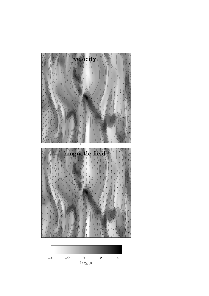
Figure 3: Two dimensional slice of increased Jeans mass model ${\cal G}i1s$ with velocity field vectors (upper panel) and magnetic field vectors (lower panel), displaying the wohle computational domain. The initial magnetic field is oriented along the $z$-direction, i.e. vertically in all plots presented. Driving happens at $k=1-2$. The field is strong enough in this case not only to prevent the cloud from collapsing perpendicular to the field lines, but even suppress the turbulent motions in the cloud. The turbulence only scarcely affects the mean field. The picture is taken at $t=5.5t_{\rm ff}$.

In a subcritical region with $M<M_{cr}$, the cloud is expected to collapse to a sheet, which in turn should be stable. Figure 3 shows the corresponding model ${\cal G}i1s$. These runs have been computed with a lower Mach number ${\cal M}=5.0$ in order to demonstrate the behavior of a magnetostatically supported cloud. The initially uniform magnetic field runs parallel to the $z$-axis. The field is strong enough to force significant anisotropy in the flow, although the dense sheets that form do not always lie perpendicular to the field lines as the driving can shift the sheets along the field lines without changing the mass-to-flux ratio. The sheets do not collapse further, because the shock waves cannot sweep gas across field lines and the cloud is initially supported magnetostatically.

Figure 4 demonstrates that this result is reasonably well resolved numerically. As in figure 1, we show peak densities and magnetic field strength for two models that differ only in their sound speeds, and thus by the number of zones in a Jeans wavelength $\lambda_{J}$. Whereas model ${\cal E}i1s$, with $\lambda_{J}=3.2$ zones does collapse, although it should be supported, model ${\cal G}i1s$, with $\lambda_{J}=6.8$ zones behaves as expected physically, just as our resolution criterion predicts. Note that the actual field strength in model ${\cal G}i1s$ always exceeds $B_{sup}$, the field strength necessary to support the region.

4.2 MHD Wave Support

A supercritical cloud with $M>M_{cr}$ is not magnetostatically supported, and could only be stabilized by MHD wave pressure, assuming ideal MHD. In this section we show that this appears to be insufficient to completely prevent gravitational collapse, although it can slow the process down.

4.2.1 Morphology

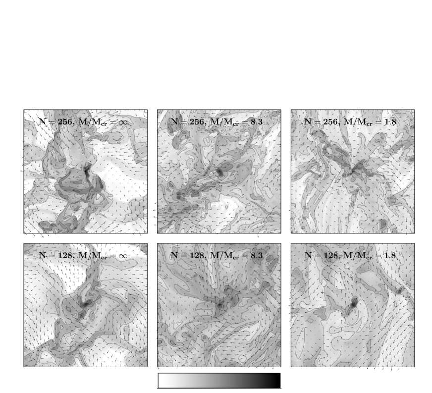
Figure 5: Two-dimensional slices of the high-resolution models ${\cal D}h1$, ${\cal E}h1w$ and ${\cal E}h1i$ and the corresponding models at intermediate resolution ${\cal D}i1$, ${\cal E}i1w$, and ${\cal E}i1i$, displaying the whole computational domain. Slices are taken at the location of the zone with the highest density at the time when $10$% of the total mass has been accreted onto cores. The plot is centered on this zone. Arrows denote velocities in the plane. The length of the largest arrows corresponds to a velocity of $v\sim 2.0$. Greyscale stands for density, where highest density regions are darkest. All slices are scaled equally, using the same scale as 3. Driving, as in figure 3, happens at $k=1-2$.

In the upper panels of Figure 5 we compare the morphology of hydrodynamical (${\cal D}h1$), weakly magnetized (${\cal E}h1w$), and strongly magnetized (${\cal E}h1i$) supercritical models at a resolution of $256^{3}$ zones. The figure presents two dimensional slices through the three dimensional simulation volume centered on the locations of the most massive clumps. In order to compare the models at similar stages of their evolution, we took the snapshots at a time when roughly 10% of the total mass had been accreted onto collapsing clumps. All three runs show well developed turbulence, rarefied regions, shocked regions, and at least one clump. However, model ${\cal E}h1w$, with $M/M_{cr}=8.3$, seems to contain more power on small scales than the pure hydro run, model ${\cal D}h1$ ($M/M_{cr}=\infty$). We discuss this more quantitatively below. In model ${\cal E}h1i$, with $M/M_{cr}=1.8$, the vertically oriented mean field (in the plane of the Figure) starts producing some anisotropy. This model represents a morphological transition from the pure hydrodynamical model ${\cal D}h1$ with completely randomly oriented motions to the magnetostatically supported model ${\cal G}i1s$, with its ordered strucures.

4.2.2 Resolution Study

We must address the question of whether our magnetodynamic simulations are indeed well resolved. The parameters for models ${\cal E}$ yield a global Jeans length of $\lambda_{J}\approx 0.5$, corresponding to a local, post-shock Jeans length of $\lambda_{J}\approx 0.05$ for isothermal shocks with Mach number ${\cal M}\approx 10$ (see Table 2). At $N=128^{3}$ zones, this results in a local Jeans length of only $3.2$ zones, but at $256^{3}$ the local Jeans length is $6.4$ zones, satisfying our resolution criterion. Instead of increasing the resolution, we increased the Jeans length in the models ${\cal G}$ discussed below in § 4.2.4 by increasing the sound speed. In these models we used a global Jeans length of $\lambda_{J}\approx 1.1$, corresponding to a local Jeans length of $6.8$ zones at $N=128^{3}$.

Figure 5 compares high resolution $256^{3}$ zone models with the corresponding lower resolution $128^{3}$ zone models in the same dynamical state, when 10% of the mass has been accreted onto cores. The lower resolution makes itself felt in broader shocks in all cases, so that the peak densities are lower than in the high-resolution runs. In the MHD models decreasing the resolution also leads to thicker collapsed sheets. Thus, unstable regions form at later times in both the MHD and hydrodynamical cases, as can be seen in Figure 6. There, we show the core mass accretion history for three weakly magnetized models varying only in their resolution ${\cal E}l1w$ ($64^{3}$), ${\cal E}i1w$ ($128^{3}$) and ${\cal E}h1w$ ($256^{3}$) (lower panel) and the corresponding hydrodynamical models (${\cal D}l1$, ${\cal D}i1$, ${\cal D}h1$) (upper panel). Cores were determined using the modified CLUMPFIND algorithm of Williams et al. (1994) as described in Paper I.

Collapse occurs in both cases at all resolutions. However, increasing the resolution makes itself felt in different ways in hydrodynamical and MHD models. In the hydrodynamical case, higher resolution results in thinner shocks and thus higher peak densities. These higher density peaks form cores with deeper potential wells that accrete more mass and are more stable against disruption. If we increase the resolution in the MHD models, on the other hand, we can better follow short wavelength MHD waves, which appear to be able to delay collapse, although not to prevent it.

The turbulent formation of gravitationally condensed regions via shock interactions is a highly stochastic process. As in Paper I, we demonstrate this by choosing different random realizations of the driving velocity field with the same characteristic wavelengths. Figure 7 shows the core mass accretion history for a pure hydrodynamical model set and a MHD set. In the upper panel, we plotted the models ${\cal D}l1$, ${\cal D}i1$, ${\cal D}h1$, where the low-resolution model ${\cal D}l1$ has been repeated multiple times (solid thin lines). The dotted thick line denotes the average of these runs. We find that resolution effects are exceeded by statistical variations caused by random variations of the driving fields.

In the MHD case (lower panel) the thickness of the lines stands for the strength of the field, expressed in terms of the ratio $M/M_{cr}$. Dotted lines denote low-resolution runs computed with varying driving velocity fields, as in the upper panel. The high-resolution run with $M/M_{cr}=1.8$ was stopped at $t=1.0t_{\rm ff}$ because the Alfvén timestep became prohibitively small. Increasing the resolution makes itself felt for the runs with stronger fields in the same way as for the ones with weak fields: The higher the resolution, the better the small-scale MHD waves are resolved, and thus the slower the collapse. Collapse does always occur, however.

4.2.3 Core Distribution

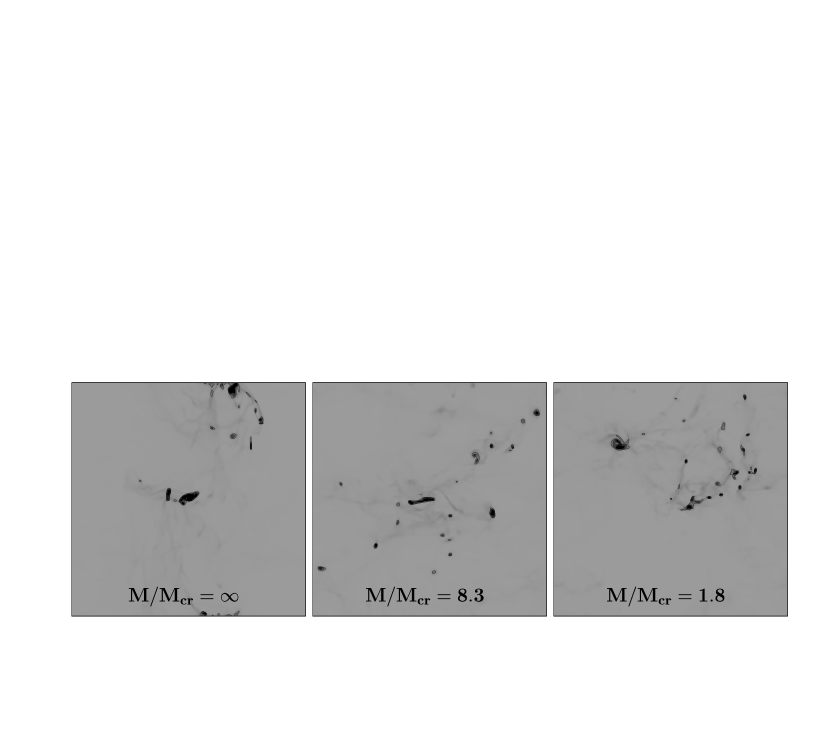
Figure 8: Projected coordinates of clumps found when $10$% of the total mass has been accreted onto cores. All simulations (models ${\cal D}h1$, ${\cal E}h1w$ and ${\cal E}h1i$) are driven at wavenumbers $k=1-2$. For the pure hydro case, we get strongly clustered collapse, whereas for supercritical fields, the cores are more evenly distributed. For slightly supercritical fields ($M/M_{cr}=1.8$, model ${\cal E}h1i$), the cloud tends to collapse along the field lines, so that the extent of the core distribution is reduced in direction parallel to the initial field (vertically oriented in the plots).

Although MHD waves cannot prevent local collapse entirely, the resulting collapse appears qualitatively different from collapse in the hydrodynamic case with corresponding global $\lambda_{J}$ and driving strength. In the hydrodynamical case driven at $\lambda_{D}>\lambda_{J}$, shocks are widely separated and sweep up substantial mass, producing isolated clusters of cores. In the presence of a weak supercritical field, the shock structure appears to have more small-scale structure, resulting in cores distributed more uniformly across the simulation volume, as shown in the middle panel of Figure 8. In fact, the weakly magnetized model driven on large scales with $\lambda_{D}>\lambda_{J}$ rather more resembles the hydro model driven on small scales with $\lambda_{D}<\lambda_{J}$ shown in Figure 11 of Paper I.

Figures 9 and 10 try to quantify this difference. Figure 9 shows the histogram of core distances for each panel of Figure 8, multiplied with the mean core mass. A clustered ensemble of high-mass cores should result in a peaked distribution at small distances, whereas a spread-out ensemble of low-mass cores should have a broader distribution. Figure 9 hints at such a behaviour, although we are well aware of the fact, that the statistics barely suffice. Nevertheless, the distribution for the magnetized runs is shifted to larger radii. Note that the total mass in the cores found is within $10$% the same for all three models. Figure 10 shows the weighted means of core distances, with their standard deviations as error bars. Again, we see a slight shift towards larger separations, suggesting a more uniform distribution of cores in the MHD cases, although larger simulations with greater core numbers will be needed to confirm this result.

4.2.4 Energy Distribution

Further evidence for a qualitative difference between hydrodynamic and MHD collapse comes from Figure 11. Here, we show the time evolution of the ratio of kinetic to potential energy, decomposed into contributions from four spatial scales. (The time resolution is somewhat coarse as these models with $256^{3}$ zones were only dumped every $t=0.3t_{\rm ff}$.) Whereas the hydrodynamic model (${\cal D}h1$) driven at $k=1-2$ collapses within less than $0.5t_{\rm ff}$, the weakly magnetized model ${\cal E}h1w$ ($M/M_{crit}=8.3$) is supported until $t\gtrsim 1t_{\rm ff}$ before also collapsing. This is at least qualitatively similar to the behavior of model ${\cal D}h3$, which is driven at wavenumbers $k=7-8$ and thus has a denser network of shocks. On the other hand, Figure 11 suggests that the stronger-field model ${\cal E}h1i$ ($M/M_{cr}=1.8$) collapses even more thoroughly than its hydrodynamical counterpart due to the ordering influence of the strong mean field.

We use the model series ${\cal G}$ to follow the collapse to later times and with more frequent time sampling. These $128^{3}$ models still resolve the Jeans length in the densest clumps, as discussed in § 4.2.2. We reduced the Mach number to ${\cal M}=5$ in order to maintain an energy input comparable to models ${\cal E}$. This decreases the rms post-shock density, so we actually expect the ${\cal G}$ series to form cores with somewhat more difficulty than the ${\cal E}$ series. Figure 12 shows the ratio of kinetic to potential energy of the magnetized models in the ${\cal G}$ series. (The hydrodynamical model ${\cal G}i1$ collapses within half a free-fall time after gravity is turned on at $t=0.0$.) With increasing field strength (models ${\cal G}i1w$ and ${\cal G}i1i$), the collapse is delayed, but never prevented. This even applies for ${\cal G}i1m$, where the field strength is only marginally supercritical ($M/M_{crit}=1.1$). In this model, bound cores form, but are then destroyed by passing shocks, probably for the unphysical reason that they cannot continue collapsing to sizes smaller than a few zones (see discussion in Paper I). Increasing the field strength further leads to model ${\cal G}i1s$ ($M/M_{crit}=0.8$), where the field supports the cloud magnetostatically, and gravitationally bound cores do not form.

4.2.5 Energy Spectra

We next examine Fourier spectra of the energy. Figure 13 presents the spectra of kinetic, potential and magnetic energies at times $t=0.0$ and $t=1.5t_{\rm ff}$ of the high-resolution models ${\cal D}h1$ (hydrodynamic), ${\cal E}h1w$ ($M/M_{cr}=8.3$) and ${\cal E}h1i$ ($M/M_{cr}=1.8$), all driven at wavenumber $k=1-2$. The spectra at time $t=0.0$ represent fully developed turbulence just before gravity is switched on. Here we find another reason for the fast collapse of the more strongly magnetized model ${\cal E}h1i$. The density enhancements due to shock interactions are larger for models ${\cal D}h1$ and ${\cal E}h1i$ than for ${\cal E}h1w$, as can be inferred from comparing the potential energies at $t=0.0$. Although still supercritical, the field in model ${\cal E}h1i$ is already strong enough to suppress motions perpendicular to the mean field, so that the field strength perpendicular to its initial mean direction is small, while strong shocks/waves can be formed parallel to the mean field, as observed as well by Smith et al. (2000). Thus, somewhat surprisingly, the density enhancements are larger for the stronger-field model ${\cal E}h1i$ than for the weak-field model ${\cal E}h1w$, leading to earlier collapse, as seen in Figure 11. In model ${\cal E}h1w$ the weaker, more turbulent magnetic field produces a more isotropic magnetic pressure that cushions and broadens the shocks, thus decreasing the density enhancements and delaying collapse.

We illustrate this effect in Figure 14, where we plot the $x$- $y$- and $z$-components of the magnetic energy against time for the magnetized models ${\cal E}h1w$ and ${\cal E}h1i$. In the weak-field case, the field is quickly tangled by the flow, so that it has no preferred direction by $t=0.0$, when gravity is switched on. The magnetic energy, and so the magnetic pressure, is isotropic. There is no secular increase of any component with time, supporting the picture of local collapse: In a globally collapsing environment, the magnetic field lines would follow the global gas flow and lead to a noticeable increase of magnetic energy. In the stronger-field case, on the other hand, the flow is dominated by the mean field oriented along the $z$-axis. The field allows matter to move more freely in the parallel than in the perpendicular direction. Matter thus collapses preferentially along field lines first, and then globally collapses.

After one free-fall time all the models have collapsed (Figure 13). Note that, as in Paper I, $E_{pot}(k)>E_{kin}(k)$ for all $k$ does not necessarily mean that the model becomes globally unstable. With increasing time, $E_{pot}(k)$ becomes constant for all $k$ just because this is the Fourier transform of a $\delta$-function, signifying that local collapse has produced point-like high-density cores. A similar argument applies for the kinetic energy: The flat spectrum stems from local concentrations of kinetic energy around the collapsing regions. Here, the spectral analysis no longer yields information on global stability.

4.2.6 Conclusions

We conclude that the delay of local collapse seen in our magnetized simulations is caused mainly by weakly magnetized turbulence acting as a more or less isotropic pressure in the gas, decreasing density enhancements due to shock interactions. We feel justified in claiming that magnetic fields, as long as they do not provide magnetostatic support, can not prevent local collapse, even in the presence of supersonic turbulence.

We note that once bound cores form, we take this as evidence for local collapse, although subsequent shock interactions may destroy these cores again. In a real cloud, ambipolar diffusion would set in at the length scale of transient cores, so that any internal turbulence would be quickly dissipated, allowing further collapse, as discussed in Paper I.

A large-scale driver, such as interacting supernova remnants or galactic shear, together with magnetic fields, seems to act like a driver with a smaller effective scale in the sense that both yield a more uniform core distribution and a somewhat slower collapse rate. In weakly magnetized turbulence, a more or less isotropic magnetic pressure reduces the density enhancements behind shocks and thus slows down the process of isolated collapse. In strongly magnetized turbulence, however, the mean magnetic field dominates. The magnetic pressure is not isotropic any more, so the shocks perpendicular to the mean field direction cause high enough density enhancements for the regions to collapse within a free-fall time.

Thus, for small field strength, the effective additional pressure may be represented by a simple pressure term. However, in the regime of field strength interesting for molecular clouds, the field, although supercritical, is strong enough to result in an anisotropic magnetic pressure. Magnetic turbulence is an all-scale non-isotropic phenomenon, and the compression and perturbations on large scales make the cloud finally collapse.

5 Summary

In this paper, we investigated whether magnetized turbulence can prevent collapse of a Jeans-unstable region. From our high-resolution simulations we conclude that

1. In order to resolve self-gravitating MHD turbulence using a grid-based method like ZEUS-3D, the local Jeans length should not fall short of at least four grid zones for magnetostatic support and six grid zones for magnetodynamic support.

2. Local collapse cannot be prevented by magnetized turbulence in the absence of mean-field support. Strong local density enhancements due to shock interactions start collapsing at once.

3. However, the magnetic fields do delay local collapse by decreasing local density enhancements via magnetic pressure behind shocks.

4. Weakly magnetized turbulence appears qualitatively similar to hydrodynamic turbulence driven on a slightly smaller scale, while stronger fields close to but under the value for magnetostatic support tend to organize the flow into sheets and allow more clustered collapse.

5. The strength and wavelength of turbulent driving governs the behaviour of the cloud, overshadowing the effects of magnetic fields that do not provide magnetostatic support.

6. MHD turbulence can not prevent local collapse for much longer than a global free-fall time. Stars begin to form at a low rate as soon as local density enhancements contract. This result favours a dynamical picture of molecular clouds being a transient feature in the ISM (Ballesteros-Paredes et al. 1999, Elmegreen 2000) rather than living for many free-fall times.

Name	Resolution	$k_{drv}$	$M_{J}^{turb}$	$\beta$	$\beta_{turb}$	$M/M_{cr}$	$t_{5\mbox{\%}}$
${\cal D}h1$	$256^{3}$	$1-2$	$15$	$\infty$	$\infty$	$\infty$	$0.4$
${\cal D}h3$	$256^{3}$	$7-8$	$15$	$\infty$	$\infty$	$\infty$	$0.7$
${\cal E}h1w$	$256^{3}$	$1-2$	$15$	$0.9$	$87.2$	$8.3$	$1.4$
${\cal E}i1w$	$128^{3}$	$1-2$	$15$	$0.9$	$87.2$	$8.3$	$1.3$
${\cal E}l1w$	$64^{3}$	$1-2$	$15$	$0.9$	$87.2$	$8.3$	$0.6$
${\cal E}h1i$	$256^{3}$	$1-2$	$15$	$0.04$	$3.9$	$1.8$	$0.8$
${\cal E}i1i$	$128^{3}$	$1-2$	$15$	$0.04$	$3.9$	$1.8$	$0.4$
${\cal E}l1i$	$64^{3}$	$1-2$	$15$	$0.04$	$3.9$	$1.8$
${\cal E}i1s$	$128^{3}$	$1-2$	$15$	$0.01$	$1.0$	$0.8$	$1.5$
${\cal E}l1s$	$64^{3}$	$1-2$	$15$	$0.01$	$1.0$	$0.8$	$1.0$
${\cal E}i0s$	$128^{3}$	$0$	$-$	$0.01$	$-$	$0.8$	$-$
${\cal E}l0s$	$64^{3}$	$0$	$-$	$0.01$	$-$	$0.8$	$-$
${\cal F}l0w$	$64^{3}$	$0$	$-$	$3\cdot 10^{-3}-0.14$	$-$	$1.10$	$-$
${\cal F}l0i$	$64^{3}$	$0$	$-$	$2\cdot 10^{-3}-0.09$	$-$	$0.88$	$-$
${\cal F}l0m$	$64^{3}$	$0$	$-$	$1\cdot 10^{-3}-0.04$	$-$	$0.59$	$-$
${\cal F}l0s$	$64^{3}$	$0$	$-$	$3\cdot 10^{-4}-0.02$	$-$	$0.44$	$-$
${\cal G}i1$	$128^{3}$	$1-2$	$19$	$\infty$	$\infty$	$\infty$	$1.2$
${\cal G}i1w$	$128^{3}$	$1-2$	$19$	$4.04$	$100.0$	$8.3$	$2.1$
${\cal G}i1i$	$128^{3}$	$1-2$	$19$	$0.23$	$5.9$	$2.0$	$1.0$
${\cal G}i1m$	$128^{3}$	$1-2$	$19$	$0.07$	$1.8$	$1.1$	$(3.5)$
${\cal G}i1s$	$128^{3}$	$1-2$	$19$	$0.05$	$1.1$	$0.8$	$-$

Table 1: Parameters of models used. $M_{J}^{turb}=\rho^{1/2}(\pi/G)^{3/2}(c_{s}^{2}+\langle v^{2}\rangle/3)^{3/2}$ gives the turbulent Jeans mass, $\beta=P_{th}/P_{mag}=8\pi c_{s}^{2}\rho/B^{2}$ and $\beta_{turb}=P_{turb}/P_{mag}$. $t_{5\mbox{\%}}$ denotes the time at which $5$% of the total mass has been accreted onto cores. Times have been normalized to the global free-fall time. $M/M_{cr}$ gives the ratio of cloud mass to critical mass according to equation 2. Models ${\cal E}l1i$ and ${\cal E}l1s$ have been computed three times with varying random seeds to check the influence of the velocity field on the results. They are not listed explicitly. Models ${\cal E}l0s$, ${\cal E}i0s$ and ${\cal F}$ are non-driven runs, used for the analysis of numerical diffusion. Model ${\cal G}i1s$ collapses so slowly, that it only reached $M_{*}=3$% after $t=3.5t_{\rm ff}$.

model	$c_{s}$	$n_{J}$	${\cal M}$	$\lambda^{pk}_{J}$	$64^{3}$	$128^{3}$	$256^{3}$
${\cal D/E}$	$0.10$	$64$	$10$	$0.05$	$1.6$	$3.2$	$6.4$
${\cal G}$	$0.213$	$6.4$	$5$	$0.11$	$3.4$	$6.8$	$13.6$

Table 2: Peak Jeans lengths for all turbulent models, where $\lambda^{pk}_{J}$ is determined via the peak density $\rho_{pk}={\cal M}^{2}\rho_{0}$. The second column lists the sound speed $c_{s}$, followed by the Mach number ${\cal M}$ and the number of thermal Jeans masses in the box $n_{J}$. The last three columns contain the Jeans lengths in zones for the resolution denoted in the top row.

Figure 1: Peak densities and maximum magnetic field strengths for strong field ($M/M_{cr}=0.8$), driven (${\cal E}l1s$ and ${\cal E}i1s$) and undriven (${\cal E}l0s$ and ${\cal E}i0s$) runs. The dotted lines (upper $N=128^{3}$, lower $N=64^{3}$) denote the sheet densities, i.e the densities corresponding to all mass concentrated in a layer of one grid zone’s height. Gravity is turned on at $t=0.0$ with $t$ in units of the global free-fall time scale $t_{\rm ff}$. The time interval at $t<0.0$ is necessary for the driven models to reach a state of fully developed turbulence. In the lower panels, the thin lines denote the magnetic field strength required to support a region of density $\rho_{max}$ according to equation 2

Figure 2: Peak densities for all test models of type ${\cal F}$. $\lambda_{J}$ is the Jeans length in units of grid zones, when all the mass is collected in a sheet of a single zone’s height. The horizontal dotted line denotes the density reached if all mass is collected in sheet of a single zone’s height. Note that for $\lambda_{J}=4.0$ zones we get collapse in the supercritical case ($M/M_{cr}=1.1$), but not in the subcritical one. Thus, we verify the mass-to-flux criterion (equation 2).

Figure 4: Peak densities and maximum magnetic field strengths for strong field model ${\cal E}i1s$ (solid line) and model ${\cal G}i1s$ (dashed line). The dotted line denote the sheet density, i.e the density corresponding to all mass concentrated in a layer of one grid zone’s height. Gravity is turned on at $t=0.0$ with $t$ in units of the global free-fall time. In the lower panel, the thin lines denote the magnetic field strength required to support a region of density $\rho_{max}$ according to equation 2. Whereas model ${\cal E}i1s$ shows unphysical, numerical collapse, model ${\cal G}i1s$ is well resolved.

Figure 6: Comparison of the mass accretion behaviour for runs driven at $k=1-2$ with varying resolution. Pure hydro runs are shown in the upper panel (models ${\cal D}l1$ (dotted), ${\cal D}i1$ (dashed), and ${\cal D}h1$ (solid)), and MHD runs are shown in the lower panel (models ${\cal E}l1$ (dotted), ${\cal E}i1$ (dashed), and ${\cal E}h1$ (solid)). $M_{*}$ denotes the sum of masses found in all cores determined by the modified CLUMPFIND (Williams et al. 1994, see also Paper I). Times are given in units of free-fall time as defined in equation 1. Although the collapse rate varies, we get collapse in all cases.

Figure 7: (Upper panel) Core-mass accretion rates for $10$ hydro runs with equal parameter set (model ${\cal D}l1$) but different realizations of the turbulent velocity field. The thick line shows a “mean accretion rate”, calculated from averaging over the sample. For comparison, the higher-resolution runs ${\cal D}i1$ and ${\cal D}h1$ are shown. The latter one ($N=256^{3}$) can be regarded as an envelope for the low resolution models. (Lower panel) Mass accretion rates for runs with identical magnetic fields but different driving fields, and runs with identical driving fields but different magnetic fields (models ${\cal E}l1w$, ${\cal E}i1w$, ${\cal E}h1w$ and ${\cal E}l1i$, ${\cal E}i1i$, ${\cal E}h1i$). The effects of magnetic fields are covered by variations due to the turbulent velocity field. Identical line styles stand for models with identical parameters, but different driving velocity fields. Models ${\cal E}l1w$ and ${\cal E}l1i$ have been computed $3$ times with varying driving velocity fields.

Figure 9: Histogram of core distances weighted with the mean core mass for the projected cores of Figure 8. The box length is $L=2$. The weighted means and their standard deviations are shown in Figure 10. Although the statistics are not sufficient, the magnetized models tend to show a more uniform distribution.

Figure 10: Weighted means and their standard deviations for the core distances of Figure 9. The effect of low number statistics is clearly to be seen (between six and ten cores were found).

Figure 11: Time evolution of the ratio of kinetic to potential energy, $T/V$ split up according to wavenumber $k=1,2,4,8$ (solid, dashed, dash-dotted and dotted lines) for models ${\cal D}h1$, ${\cal D}h3$ (driven at $k=7-8$), ${\cal E}h1w$ and ${\cal E}h1i$. The horizontal line at $T/V=1.0$ indicates the instability boundary. Time is normalized to units of global free-fall time $t_{ff}$. Note that a strong subcritical field leads to faster collapse than a weak subcritical one.

Figure 12: Ratio of kinetic to potential energy against time for models ${\cal G}$ with reduced number of Jeans masses ($n_{J}=6.4$), split up into contributions from four spatial scales ($k=1,2,4,8$). All models show collapse except for the magnetostatically supported one (${\cal G}i1s$). Note that models ${\cal G}i1w$ and ${\cal G}i1i$ behave as their counterparts ${\cal E}h1w$ and ${\cal E}h1i$ shown in figure 11.

Figure 13: Kinetic, potential and magnetic energies for models ${\cal D}h1$ ($k=1-2$, $M/M_{cr}=\infty$), ${\cal E}h1w$ ($k=1-2$, $M/M_{cr}=8.3$) and ${\cal E}h1i$ ($k=1-2$, $M/M_{cr}=1.8$) at the time $t=0.0$ at which gravity is turned on in a state of fully developed turbulence (upper row). For comparison we included power spectra of $P(k)\propto k^{-5/3}$ and $P(k)\propto k^{-2}$ (dotted lines). The lower row contains the same models, but for time $t=1.0t_{\rm ff}$.

Figure 14: Magnetic energy components for magnetic models ${\cal E}h1w$ (thick lines) and ${\cal E}h1i$ (thin lines) against time. Solid lines denote the energy of the $z$-component (initial mean field orientation), dashed lines the $x$- and $y$-components. Gravity is turned on at $t=0.0$. In the weakly magnetized model ${\cal E}h1w$, the field has ceased to show a net orientation at $t=0.0$. It has developped a fully turbulent state. The strong field (${\cal E}h1i$) continues to keep its mean orientation.

References

- (1) Ballesteros-Paredes, J., Hartmann, L., Vázquez-Semadeni, E. 1999 ApJ, 527, 285
- (2) Bate, M. R., & Burkert, A. 1997, MNRAS, 288, 1060
- (3) Blitz, L., Shu, F. H. 1980, ApJ, 238, 148
- (4) Burkert, A. & Bodenheimer, P. 1993, MNRAS, 264, 798
- (5) Clarke, D. 1994, National Center for Supercomputing Applications Technical Report
- (6) Crutcher, R.M. 1999, ApJ, 520, 706
- (7) Dewar, R.L. 1970, Phys. Fluids, 13, 2710
- (8) Elmegreen, B. 2000, ApJ, 530, 277
- (9) Evans, C., Hawley, J.F. 1988, ApJ, 33, 659
- (10) Fiege, J.D. & Pudritz, R.E. 1999, in New Perspectives on the Interstellar Medium, ASP Conference Series 168, edited by A. R. Taylor, T. L. Landecker, and G. Joncas, 248
- (11) Gammie, C. F., Ostriker, E. C. 1996, ApJ, 466, 814
- (12) Hawley, J. F., Stone, J. M. 1995, Comp. Phys. Comm. 89, 127
- (13) Hennebelle, P., & Pérault, M. 1999, A&A, 351, 309
- (14) Hildebrand, R.H., Dotson, J.L., Dowell, C.D. et al. 1999, ApJ, 516, 834
- (15) Klessen, R.S., Heitsch, F., Mac Low, M.-M. 1999, ApJ, 535, 887
- (16) Klessen, R.S., & Burkert, A., 2000, ApJS, 128, 287
- (17) Mac Low, M.-M., Klessen, R. S., Burkert, A., Smith, M. D. 1998, Phys. Rev. Lett., 80, 2754
- (18) Mac Low, M.-M., 1999, ApJ, 524, 169
- (19) Matthews, B.C., & Wilson, C.D., 2000, ApJ, 531, 868
- (20) McKee, C.F. 1999, in The Origin of Stars and Planetary Systems, edited by Charles J. Lada and Nikolaos D. Kylafis. Kluwer Academic Publishers, 1999, p.29
- (21) McKee, C.F. & Zweibel, E.G. 1995, ApJ, 440, 686
- (22) Mouschovias, T.C. & Spitzer, L. 1976, ApJ, 210, 326
- (23) Nakano, T. & Nakamura, T. 1978, PASJ, 30, 681
- (24) Nakano, T. 1998, ApJ, 494, 587
- (25) Ostriker, E. C., Gammie, C.F., Stone, J. M. 1999, ApJ, 513, 259
- (26) Padoan, P., Nordlund 1999, ApJ, 526, 279
- (27) Shu, F.H., Adams, F.C., Lizano, S. 1987, ARA&A, 25, 23
- (28) Smith, M., MacLow, M.-M., Heitsch, F. 2000, A&A, in press
- (29) Stone, J. M., & Norman, M. L. 1992a, ApJS, 80, 753
- (30) Stone, J. M., & Norman, M. L. 1992b, ApJS, 80, 791
- (31) Stone, J. M., Ostriker, E. C., Gammie, C. F. 1998, ApJ, 508, L99
- (32) Truelove, J. K., Klein, R. I., McKee, C. F. et al. 1997, ApJ, 489, L179
- (33) Vázquez-Semadeni, E., Gazol, A. 1995, A&A, 303, 204
- (34) Vázquez-Semadeni, E., Passot, T., Pouquet, A. 1996, ApJ, 473, 881
- (35) Vázquez-Semadeni, E. et al. 2000, in Protostars and Planets IV, eds. V. Mannings, A. Boss & S. Russell, p.3
- (36) Williams, J. P., De Geus, E., Blitz, L. 1994, ApJ, 428, 693
- (37) Williams, J. P., Blitz, L., McKee, C. F. 2000, in Protostars and Planets IV, eds. V. Mannings, A. Boss & S. Russell, p.97