Superclustering of Faint Galaxies in the Field of
a QSO Concentration at $z\sim 1.1$

Abstract

We report on a wide-area ($48^{\prime}\times 9^{\prime}$) imaging survey of faint galaxies in $R$ and $I$ bands toward the 1338+27 field where an unusual concentration of five QSOs at $z\sim 1.1$, embedded in a larger-scale clustering of 23 QSOs, is known to exist. Using a quite homogeneous galaxy catalog with a detection completeness limit of $I\sim 23.5$, we detect a significant clustering signature of faint red galaxies with $I>21$ and $R-I>1.2$ over a scale extending to $\sim 20h^{-1}_{50}$ Mpc. Close examination of the color-magnitude diagram, the luminosity function, and the angular correlation function indeed suggests that those galaxies are located at $z\sim 1.1$ and trace the underlying large-scale structure at that epoch, together with the group of 5 QSOs. Since the whole extent of the cluster of 23 QSOs ($\sim 70h^{-1}_{50}$ Mpc) is roughly similar to the local “Great Wall”, the area may contain a high-redshift counterpart of superclusters in the local universe.

1 Introduction

Superclusters are the largest recognizable structures in the universe, and thus retain the imprint of primordial density fluctuations in a fairly direct manner. Due to several observational difficulties in detecting such weak clustering over large scales at higher redshifts, however, only a few superstructures at $z>0.5$ are currently identified (e.g. Connolly et al. 1996; Lubin et al. 2000). Oort, Arp, & de Riter (1981) pointed out that concentrations of QSOs/AGNs, which are relatively easy to identity, may be possible sites for such superclusters at higher redshifts.

Crampton et al. (1988, 1989) discovered an unusual concentration of 23 QSOs at $z\sim 1.1$ in $\sim 2.2\times 2.2$ deg² field denoted as 1338+27. Subsequent observations by Hutchings et al. (1993, 1995) and by Yamada et al. (1997) revealed an excess of faint galaxies near several QSOs in the concentration. These findings suggest either that the QSOs are located in isolated rich associations of galaxies or that those QSOs and the galaxies trace the underlying large-scale structure in a similar manner. While either interpretation has an interesting implication for the origin and evolution of spatial biasing of QSOs and galaxies at high redshifts, previous observations are not able to discriminate between the above two possibilities due to the limited size of the observed fields. We carried out a new deep optical imaging observation of galaxies in the $48^{\prime}\times 9^{\prime}$ region including the highest density peak of the QSO concentration at $z=1.1$, and found that there are several concentrations of galaxies whose color and magnitude are consistent with old galaxies at $z\sim 1.1$. While they do not seem to be directly associated with any particular QSO, they show clustering over the entire QSO group in our observed area. This indicates that both those galaxies and QSOs are the tracers of much larger-scale structure (possibly even as large as the whole cluster scale of 23 QSOs), perhaps similar to the “Great Wall” in the local universe (de Lapparent, Geller, & Huchra, 1986).

The rest of this paper is organized as follows. After briefly describing our observations and data reduction in §2, we present the results of an object finding analysis and the resulting density map (§3.2). The color-magnitude diagram and the luminosity function for the detected high-density regions are considered in §3.3. A further analysis by angular correlation functions for the whole survey region is described in §3.4. Finally we summarize our findings and discuss their interpretation and implications in §4. We assume the Hubble constant $H_{0}=50$km/s/Mpc, the density parameter $\Omega_{0}=1$, and the cosmological constant $\Lambda=0$ throughout the paper.

2 Deep imaging of galaxies near the 1338+27 field

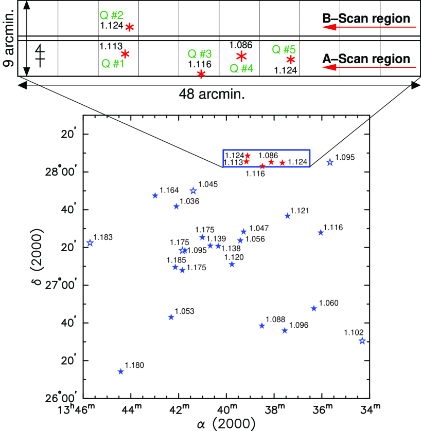
Figure 1: Top: The configuration of our $48^{\prime}\times 9^{\prime}$ TDI survey region in the 1338+27 field. The location of the five QSOs with their redshifts are shown by asterisks. B2 1335+28, the only radio-loud QSO in the area, is “Q#4”. The “A-Scan” region is characterized by the fact that the area contains four of the five QSOs. The whole scan-length of 48’ corresponds to $24.7h_{50}^{-1}$ Mpc at $z=1.1$. Bottom: Wide-area view of the concentration of 23 $z\sim 1.1$ QSOs in the 1338+27 field. The original members of the QSO cluster identified by Crampton et al. (1989) are shown by filled stars, whereas some other QSOs at $1.0<z<1.2$ in the area (their redshifts are determined and supplied to the NASA Extragalaxtic Database (NED) after the publication of the paper) are represented by open stars with their redshifts. Our survey field is indicated by the box.

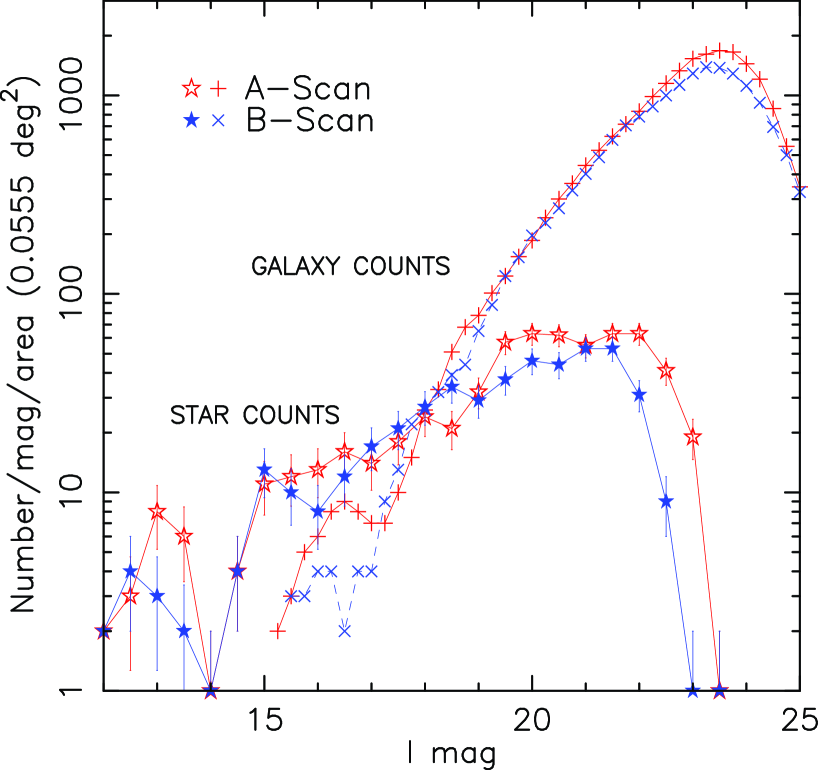
Figure 2: Results of the star counts (open and filled stars) and the galaxy number counts (pluses and crosses) for the A- & B-Scan regions.

We observed the $48^{\prime}\times 9^{\prime}$ region around the highest density peak of five QSOs in the 1338+27 field (Fig. 2 of Crampton et al. 1989) in Kron-Cousins–like R and I bands on Feb 23 to 25, 1998 using the SPIcam instrument on the 3.5-meter telescope at the Apache Point Observatory (APO). We obtained the images of the two adjacent scan regions (Fig. 1) where the group of the five QSOs at $z\sim 1.1$ (Crampton et al., 1989) exists; four of them are located in the A-scan (QSO #1 at $z=1.113$, #3 at $z=1.116$, #4 at $z=1.086$ and #5 at $z=1.124$), and the other one in the B-scan (QSO #2 at $z=1.124$). The observations were performed in TDI (time-delay–and–integrate) mode with a scanning speed of 0.2 times sidereal, i.e., $3^{\prime\prime}$/second. We operated the SPIcam in the $2\times 2$ binning mode, and the resulting pixel size and the field of view of each frame are 0.282^′′ and $4^{\prime}.78\times 4^{\prime}.78$, respectively. The net integration time for each object in a scan is thus 96 seconds, and we repeated the scans of both A and B regions five times in each band. The sky was almost clear and photometric during the exposures and the seeing was $1.2^{\prime\prime}\sim 1.5^{\prime\prime}$. Details of the reduction procedures are described in Tanaka (2000).

After flat-fielding orthogonal to the scanning direction, we obtained $R$ and $I$ images with superior homogeneity across the whole area. Object detection and photometry used the SExtractor package ver 2.0 (Bertin & Arnouts, 1996). We executed detection on the $R$ and $I$ combined frame with a detection threshold of $2.1\sigma$ and with a $3\times 3$ top-hat convolution kernel. We adopted the SExtractor “MAG_BEST” output as the “total” magnitude of objects, while we measured the color of objects on the seeing-matched registered frames using a fixed circular aperture with $2.8^{\prime\prime}$ diameter. We performed the photometric calibration using our calibrated deep images taken with the Issac Newton Telescope (Yamada et al., 1997; Tanaka et al., 2000) whose observed field significantly overlaps that of the current survey. Unsaturated and compact objects (mostly stars) detected in both images were used for the photometric calibration.

In Figure 2, we show the galaxy number counts as well as the star counts in each scan region. We classify objects as “stars” when SExtractor the “stellarity” index is over 0.90. Figure 2 shows that the star-galaxy classification is mostly complete up to $I\sim 22$. In total, we have detected 10370 objects among which 584 objects are classified as stars and removed from the analysis below.

Although the star counts in the A-Scan region are systematically higher than those in the B-Scan below $I\sim 22$ mag., which may be due to the slightly different seeing size, the effect of the mis-classification on our analysis below is estimated to be negligible since the source counts at such faint magnitude are dominated by galaxies.

The “turn-around” magnitude in the galaxy number counts is around $I\sim 23.5$ for both the scans. The good agreement of the counts in the two scan regions indicates that the quality of the images is globally the same. There is a slight excess of the number of faint galaxies in the A-Scan below $I=22$ mag. It is partially due to the effect of a rich clusters of galaxies near the eastern edge in the A-Scan and partially due to the population of galaxies studied in this paper.

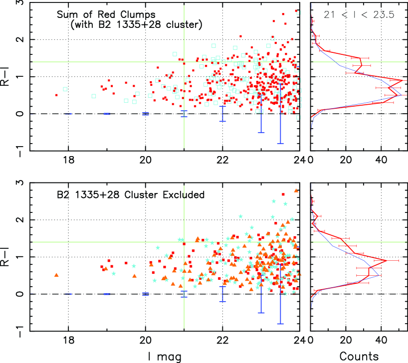
Figure 5: Top: Color-magnitude diagram for the galaxies in the four $2\arcmin.4\times 2\arcmin.4$ regions around the clumps exceeding $2.5\sigma$ density in Fig. 4 (cl_1, cl_2, cl_3, & cl_5). Open squares indicate galaxies in cl_2, a known rich cluster near B2 1335+28 (Q #4). The position of $R-I=1.4$ and $I=21$ are marked by thin lines for clarity. The error-bars plotted on the $R-I=0$ line are estimated for galaxies with $R-I=1$ from our simulation. The right panel shows the projected color distributions for galaxies with $21<I<23.5$ with $\Delta(R-I)=0.2$ bins (thick lines with errorbars). The histogram with thin lines indicates the expected average counts obtained using the whole B-Scan region. Poisson error-bars are assumed in the histogram. Bottom: The same as the upper panel, but the cluster around B2 1335+28 is excluded and the galaxies in each clump are shown in different symbols (squares for cl_1, stars for cl_3, and triangles for cl_5).

Since we focus on the difference between the A-Scan (QSO clustered area) and the B-Scan (comparison field) regions in the analysis below, we carefully compared the detection efficiency of the two scans using simulations of artificial objects (Tanaka 2000) and confirmed that the object detection in both scans is quite homogeneous up to the nominal completeness limit of $I\sim 23.5$. The photometric accuracy is evaluated as $\approx 0.2$ mag at $I\sim 22.5$ mag and $\approx 0.5$ mag at $I\sim 23.5$ mag (see errorbars in Fig. 5), and is almost the same in each scan. Magnitudes of objects in the overlapped region of the A-Scan and the B-Scan were also examined. They agree with an r.m.s. of $\mathrel{\hbox{\hbox to0.0pt{\hbox{\lower 4.0pt\hbox{$\sim$}}\hss}\hbox{$<$}}}0.05$ magnitude.

3 Detection of clustering of faint galaxies in the field

3.1 Expected galaxy colors and magnitudes at $z=1.1$

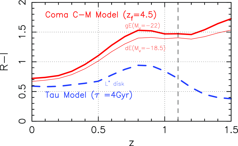
Figure 3: Predicted evolution of the $R-I$ color for model galaxies. Thick and thin solid curves correspond to the passively-evolving giant and dwarf elliptical models with $M_{V}$ of each $-22$ and $-18.5$ at the age of 12 Gyr (we assume the formation redshift of $z_{f}=4.5$) calibrated for the color-magnitude relation of the Coma cluster. Dashed curve indicates the model galaxy with star-formation rate $\propto\exp(-t/\tau)$ and $\tau=4$ Gyr with the formation epoch of $z_{f}=4.5$.

Since we do not have the redshift of each identified object, the projection along the line of sight significantly weakens the signature of the possible clustering of objects at $z\sim 1.1$. Thus we select candidates in the corresponding redshift range according to their color and magnitude. Figure 3 plots the color tracks of model galaxies as a function of redshift calculated on the basis of a spectral synthesis model by Kodama & Arimoto (1997). In the figure, solid lines labeled as “Coma C-M model” indicate the models of passively-evolving old galaxies. They are calibrated by the color-magnitude (C-M) relation of the Coma cluster and are known to reproduce the evolutionary trend of the cluster early-type galaxies up to $z\sim 1.2$ (Bower, Kodama, & Terlevich, 1998; Stanford, Eisenhardt, & Dickinson, 1998; Kajisawa et al., 2000b). The dashed line labeled “Tau Model” corresponds to a model with star formation rate $\propto\exp(-t/\tau)$ and $\tau=4$ Gyr, which may be appropriate for late-type disk galaxies (Lilly et al., 1998).

Figure 3 indicates that the color criterion $1.4\mathrel{\hbox{\hbox to0.0pt{\hbox{\lower 4.0pt\hbox{$\sim$}}\hss}\hbox{$<$}}}R-I\mathrel{\hbox{\hbox to0.0pt{\hbox{\lower 4.0pt\hbox{$\sim$}}\hss}\hbox{$<$}}}1.5$ is suitable to photometrically select passively-evolving old galaxies at $z\mathrel{\hbox{\hbox to0.0pt{\hbox{\lower 4.0pt\hbox{$\sim$}}\hss}\hbox{$>$}}}0.7$. We also calculate the apparent magnitude for the “gE” model galaxy ($M_{V}=-22$ mag. at 12-Gyrs old or $z=0$). It monotonically decreases and becomes $I=21.5$ mag at $z=1.1$. Considering these models as well as the photometric uncertainties, we finally set two photometric criteria, $1.2<R-I<1.6$ & $I>21$, to extract cluster galaxies at $z\sim 1.1$ from the whole sample.

We note that there are several observational supports for the criterion that we adopt here. Tanaka et al. (2000) show that the brightest galaxy seen in the color-magnitude sequence of the cluster around B2 1335+28 at $z\sim 1.1$ (Q#4 in Fig. 1) has $I=21.4$ and $R-I=1.44$. The color and magnitude of the spectroscopically-confirmed brightest galaxies in the two clusters at $z\sim 1.26$ and $1.27$ studied by Rosati et al. (1999) would have $R-I\approx 1.5$ and $I\sim 20.5$ if they were at $z=1.1$. Star-forming galaxies at $z\sim 1$ studied by Le Fèbre et al. (1994) have magnitudes $I>21$ and converted colors of $R-I\mathrel{\hbox{\hbox to0.0pt{\hbox{\lower 4.0pt\hbox{$\sim$}}\hss}\hbox{$>$}}}1$.

3.2 Surface density map of the observed area

The Top panel of Figure 4 shows the map of identified objects satisfying the criteria $1.2<R-I<1.6$ and $21<I<23.5$. The faintest end, $I=23.5$ is the nominal completeness limit of the data. While this map already suggests that the clustering of those galaxies is weakly correlated with the locations of the QSOs as a whole, this feature is visually more significant from the density map (the Bottom panel). The latter map is constructed from galaxy number counts on regular meshes whose size is $100\times 100$ pixels² $=28^{\prime\prime}\times 28^{\prime\prime}$ with additional Gaussian smoothing with a rms of 100 pixels to “clean” the small-scale clustering in the map (see Tanaka 2000 for further details).

The most distinctive excess in the bottom panel is at around QSO #4. In fact this clump corresponds to the cluster at $z\sim 1.1$ identified previously by Yamada et al. (1997) and Tanaka et al. (2000), and its richness is at least between those of the Virgo and the Coma clusters. For reference, the expected number of $R\geqq 0$ clusters at $0.7<z<1.3$ in the area is less than unity at this depth (Postman et al., 1996).

To check whether these red galaxy clumps are consistent with clusters at $z=1.1$, we identify the most significant ones ($\mathrel{\hbox{\hbox to0.0pt{\hbox{\lower 4.0pt\hbox{$\sim$}}\hss}\hbox{$>$}}}2.5\sigma$) and then closely examine the color and magnitude distribution of galaxies in these regions. There are five clumps above this threshold as labeled in Figure 4.

We found that the clump labeled as “cl_4” has galaxies systematically bluer and brighter than the others and therefore concluded that cl_4 clump is likely to be a foreground cluster (probably at $z\sim 0.7$) which is not well distinguished from the $z=1.1$ system by our selection criteria. Indeed, the brightest red galaxy in the clump has $I=20.3$. We thus neglect this clump in all further analysis.

Assuming that the remaining four clumps of red galaxies are located at the same redshift of $z=1.1$ (see next subsections for the further discussion), we estimated their richness. Here we used the $N_{0.5}$ parameter of Hill & Lilly (1991), the number of galaxies in the magnitude range between $m_{1}$ and $m_{1}+3$ within a 0.5 Mpc radius around the cluster.

The results are summarized in Table 1. Column 2 shows the results for the whole sample of galaxies after the field correction using the counts in the whole B-Scan region where no conspicuous density excess exists. Poisson errors are assumed. Column 3 shows the results for the red-galaxy subsample with $0.8<R-I<2.0$. The color selection helps reducing the uncertainly of the field correction since the majority of the cluster galaxies at $z=1.1$ are expected to lie within this color range (note however that this choice may exclude some star-forming very blue galaxies: see Fig. 3). Column 4 is the estimated Abell richness class based on the calibration by Hill & Lilly (1991). Note that the magnitude range is very close to our completeness limit, so the actual $N_{0.5}$ value could be slightly larger than those derived from our data.

Table 1 shows that those red clumps generally have Abell richness class $\sim 0-1$ and may be relatively poor clusters except for cl_2. Since cl_2, near QSO#4, shows fairly lumpy and extended structure, we also estimate $N_{0.5}$ in the area centered on the QSO (the third row). The area does not overlap with cl_2 region, but the count is still large. These results agree with those in Tanaka et al. (2000) based on deeper images of this small region.

3.3 Color-magnitude relation and luminosity function of the detected galaxy clumps

In order to make sure that the visual clustering pattern in Figure 4 is indeed associated with galaxies located at $z\sim 1.1$, we have to show that their colors and magnitudes are consistent with those expected for the galaxies at that redshift.

The combined C-M diagram is plotted in Figure 5. All the galaxies located on the $500\times 500$ pixel² area ($=1.2\times 1.2h_{50}^{-2}$ Mpc²) around the four clumps defined in the previous section are shown in the upper panel. Galaxies in the richest clump cl_2 are shown in open squares, while the others are indicated by filled circles. A distinctive sequence around $R-I=1.4-1.6$ is clearly seen in the diagram, which shows excellent agreement with the expected color of passively-evolving old galaxies at $z\sim 1.1$ (the horizontal line). Even if we exclude the contribution of the richest clump (the lower panel) the red sequence can be recognized clearly. We also see that there is no systematic difference in the colors of the red sequence among these three clumps.

Next we examine the luminosity function (LF) of the galaxies in the clumps. The LFs of $I$-band selected “red” galaxies in the CFRS (Lilly et al., 1995) are fitted by the Schechter form (Schechter 1976) with $M^{*}_{B}=-22.89$ for a $0.75<z<1.00$ sample. The extrapolation of the Virgo cluster LF ($M^{*}_{B}=-21.4$: Sandage et al.1985; Colles 1989; Lumsden et al.1997) assuming passive evolution predicts $M^{*}_{B}=-22.9$ at $z=1.1$. Note that De Propris et al.(1999) and Kajisawa et al.(2000a) showed that the $m^{*}$ value in near-infrared $K$-band LFs for clusters at $z<1$ is fully consistent with passive evolution.

We now wish to compare these $M^{*}_{B}$ values with those of the galaxies in the four red clumps detected in our survey. Assuming that they are all located at the same redshift, we combine the data of all the clumps and fit them to the Schechter function. In order to reduce the uncertainty in the field correction, we again use the “red galaxy” sample ($R-I>0.8$) for the analysis (Note that our applied color criteria is similar to the criteria used for “red” galaxies in the CFRS). The field correction is made using the counts of the B-Scan region. Since our data are not sufficiently deep to allow a fit of the faint-end slope $\alpha$ and $M^{*}$ simultaneously, we fix the slope at $\alpha=-0.9$ following De Propris et al.(1999) and Kajisawa et al.(2000a) and then calculate the best-fit value of $M^{*}$.

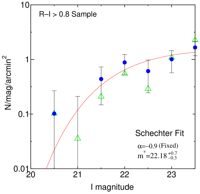
Figure 6: The luminosity function of red ($R-I>0.8$) galaxies in the fields around four $>2.5\sigma$ over-density regions. Filled circles indicate results with a rich cluster around Q #4 (B2 1335+28), while open triangles correspond to those without it. The solid curve indicates the best-fit Schechter function with a fixed slope of each $\alpha=-0.9$.

Figure 6 shows the results. For comparison, the luminosity function of galaxies excluding those in the richest clump cl_2 is also plotted in open triangles. The counts for each clump are also summarized in Table 2. The standard $\chi^{2}$-fit to the Schechter function yields $m^{*}(I)=22.18^{+0.7}_{-0.3}$ for the combined sample. Using the SED template of the passive evolution model with 3.25 Gyr old galaxies at $z=1.1$, this translates to an absolute $B$-band magnitude of $M^{*}_{B}=-22.99$. Our $M^{*}_{B}$ value agrees with the result of CFRS as well as that expected from the local cluster LF, which clearly supports the idea that these clumps of red galaxies are located at $z\sim 1.1$, the same redshift as the QSO group.

3.4 Angular correlation function

Lastly we investigate the clustering of the faint galaxy population more quantitatively using the angular two-point correlation function $\omega(\theta)$. For this purpose, we construct several color-selected subsamples, and compute the auto-correlation functions of each subsample, $\omega_{ii}$, and the cross-correlation functions between two different subsamples of galaxies, $\omega_{ij}$. We use the Landy & Szalay (1993) estimator for the former, $\omega_{ii}(\theta)=(DD_{ii}-2DR_{ii}+RR_{ii})/RR_{ii}$, and $\omega_{ij}(\theta)=DD_{ij}/RR_{ij}-1$ for the latter, where $DD$, $RR$, and $DR$ are the data-data, random-random, and data-random pairs of separation between $\theta-d\theta/2$ and $\theta+d\theta/2$, and the subscripts $i$ and $j$ refer to different subsamples. Error-bars are calculated by the standard boot-strap resampling method with 100–500 random resamplings (e.g. Barrow, Bhavsar, & Sonoda 1984). We did not apply the integral constraint correction or the correction for star-galaxy misclassification (e.g. Postman et al. 1998), since our analysis is based on the inter-comparison of signals between the A-Scan and the B-Scan regions. We note that both corrections tend to enhance the amplitude of the measured correlation signal, albeit only slightly.

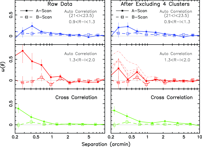
Figure 7: Angular correlation function of faint galaxies in our survey. Solid and dashed lines correspond to results for A-scan and B-scan, respectively. Left and right panels show the results with and without the four galaxy clump regions, respectively. The top and middle panels plot the auto-correlation of blue ($0.9<R-I<1.3$) and red ($1.3<R-I<2.0$) galaxies, respectively, while the bottom panels plot the cross-correlation of blue and red galaxies. Thin dot-dashed lines in the middle-right panel indicates the decreasing trend of auto-correlation signal with excluding four $>2.5\sigma$ clumps one by one.

The resulting angular correlation functions are plotted in Figure 7. Solid and dashed lines correspond to the results for the A-Scan and the B-Scan, respectively. While the clustering amplitudes for such faint galaxies are generally very weak, we see a strong signal for red ($1.3<R-I<2.0$) galaxies in the A-Scan region (the middle-left panel in Figure 7). This is in marked contrast with blue galaxies ($0.9<R-I<1.3$) which do not show appreciable auto-correlation anywhere. A similar color-selected correlation study by Woods & Fahlman (1997), whose sample has a similar depth and width to our data, showed that $\omega(\theta)$ for the red ($R-I>1$ or $>1.5$) galaxy subsample is $\sim 0.005$ at $\theta=35$ arcsec. Our result for the red ($1.3<R-I<2.0$) galaxy subsample in the B-Scan region and the blue ($0.9<R-I<1.3$) galaxy subsample agrees with their result within the errors. In contrast, our detected signal for the A-Scan region is an order of magnitude stronger than that in such typical fields.

Since the clustering signal for red galaxies becomes significantly weaker when we exclude the contribution of the four clumps (by removing the galaxies within a 1.2-Mpc radius for the richest cl_2 and a 0.6-Mpc radius for the others), it is indeed caused by the existence of these high-density clumps. The thin dot-dashed lines in the middle right panel show the systematic trend of the decreasing clustering signal as the clumps are removed one-by-one. A large decrease occurs when we exclude the cl_2 area, but a still significant clustering amplitude remains from the contribution of the other three clumps.

We also detect a slightly weaker but robust cross-correlation between blue and red galaxies, which is insensitive to the presence of the four clumps. Although we examined cross-correlations for the various color ranges, we did not find a similar signal between the other subsamples. Since the cross-correlation persists between the $0.9<R-I<1.1$ and $1.4<R-I<2.0$ subsamples, this cannot be ascribed to scatter of the observed color (due to photometric errors) of the red objects. This indicates that the A-Scan region contains a clustering of very red galaxies and somewhat bluer galaxies. The color range showing the signal corresponds to early-type ellipticals ($1.3<R-I<2.0$) and the mildly star-forming normal spiral galaxies ($0.9<R-I<1.3$) at $z=1.1$. One would normally expect that the majority of galaxies with bluer colors would be in the foreground of these red galaxies (see Fig. 3) and would not yield a significant cross-correlation signal. Further analysis indicates that this surprising signal may not be localized in any one area of the A-Scan region but rather is due to a diffuse structure extended over the whole region (Tanaka 2000).

4 Conclusions and discussion

We have detected a strong clustering signal for the faint red galaxies in the $48^{\prime}\times 9^{\prime}$ region around a tight group of five QSOs in the 1338+27 field. This structure does not seem to be confined to regions adjacent to each QSO (see Fig. 4), but rather preferentially exists only in the A-Scan region where four of the five QSOs lie; it might even extend over the entire 23 QSO concentration at $z\sim 1.1$. The color-magnitude relation, the luminosity function and the angular correlation functions of those faint galaxies consistently indicate that the clustered galaxies are located at a similar redshift to the QSO concentration. This suggests that those galaxies together with the five QSOs may both trace underlying large-scale cosmic structure at $z\sim 1.1$.

The elongated morphology and size of $\sim 2$ by $20h^{-1}_{50}$ Mpc of the structure is indeed typical of the known superclusters at low and intermediate redshifts. Jaaniste et al. (1998) studied a sample of 42 low-redshift ($z<0.12$) superclusters and concluded that elongated filamentary morphology with a size of few Mpc by several tens of Mpc is typical for the poor ($N_{cl}<8$) superclusters. There are also examples of superclusers at intermediate redshift: The cl0016 supercluster at $z\sim 0.54$ identified in Koo et al.(1985) has a thin sheet-like structure with a size of 62 by 24 by $8h_{50}^{-1}$ Mpc (Connolly et al. 1996). The supercluster at $z\sim 0.9$ studied by Lubin et al.(2000) also has an extent of $\sim 10h_{50}^{-1}$ Mpc. However, the $z=1.26$ system investigated by Rosati et al.(1999) has a projected scale of only $\sim 2h_{50}^{-1}$ Mpc.

In addition to the strong auto-correlation signal of the red galaxies in the four highest density clumps, we have also found a weak but persistent cross-correlation between blue and red galaxies. It is not caused by the galaxies in the regions of the four clumps alone but is likely to come from the whole A-Scan region. We speculate that if the structure in our surveyed region is really a supercluster at $z=1.1$, the significant cross-correlation between blue and red galaxies may originate from the association of early-type galaxies and relatively blue disk galaxies in groups distributed between the four richest clumps of red galaxies. In nearby cosmic structures such an association is typically seen(Postman & Geller, 1984; Zabludoff & Mulchaey, 1998). Indeed, Davis & Geller (1976) also detected a significant angular cross-correlation between ellipticals and spiral galaxies using a large-area catalog that contains the Local Supercluster.

Finally, we also briefly discuss the immediate environment of the five individual QSOs. QSO#4 (B2 1335+28) is the only radio-loud quasar (RLQ) in our field. Although RLQs often reside in the central regions of clusters (e.g. Ellingson & Yee 1994), Sánchez & González-Serrano (1999) found that several RLQs at $z>1$ are also located in the outskirts of cluster regions. In our case, Tanaka et al.(2000) showed that QSO#4 also resides on the northern edge of the distribution of the cluster galaxies.

A possible association of a low-significance (2 $\sigma$) clump of red galaxies with a radio-quiet QSO (RQQ) Q#1 is seen in the density map of Figure 4. Indeed, Hutchings et al. (1995) argued that there is a 3-$\sigma$ excess of faint (but $I\mathrel{\hbox{\hbox to0.0pt{\hbox{\lower 4.0pt\hbox{$\sim$}}\hss}\hbox{$<$}}}22$) blue ($R-I<1.0$) galaxies in this location. They also detected some emission-line galaxy candidates around QSOs #1 and #2. We examined the C-M diagram of the galaxies around the density peak near Q#1. Sequences of galaxies can be recognized around $R-I=1.1-1.3$ and $R-I\sim 0.7$ but they are too blue to be old passively-evolving galaxies at $z=1.1$. Furthermore, the brightest galaxy in the redder C-M sequence, which lies at the center of the clustering, has $I=19.5$ and therefore is too bright for a quiescent brightest cluster galaxy at $z=1.1$. Thus, the weak density excess in the red galaxy distribution near QSO#1 may be a chance projection of a foreground cluster, while our data do not rule out the existence of a group of blue galaxies associated with QSO #1. There is no significant density peak coincident with QSO#2, QSO#3, or QSO#5

Thus, all four RQQs seem not to be associated directly with rich clusters/groups. It is generally believed that RQQs avoid cluster environments and are fairly isolated (Yee & Green, 1984; Boyle & Couch, 1993; Teplitz, McLean, & Malkan, 1999). Our result agrees with the general trend, even though our RQQs are strongly clustered. When we consider the distribution of the QSOs and the clumps of red galaxies globally, however, we note that RQQs may preferentially reside farther into the outskirts of galaxy clusters. Yee (1990) also reported such a trend based on a study of low-redshift RQQ environments.

To date there have been only a few other observational attempts to directly relate the clustering of AGNs and superclusters (Ford et al. 1983; Longo 1991; Ellingson & Yee 1994). On the other hand, several extensive studies searching for large-scale clustering of QSOs/AGNs have already been performed (e.g. Oort et al. 1981; West 1991; Graham, Clowes, & Campusano 1995; Komberg, Kravtsov, & Lukash 1996). More homogeneous samples of such AGN groups/clusters are likely to be constructed from the 2dF QSO survey and the Sloan Digitized Sky Survey. Clearly, more extensive studies that determine the relationship of such AGN groups and superclusters to underlying large scale structure are of great importance.

The detected signature of the putative supercluster at $z=1.1$ may be the first direct indication of the association of QSOs and a high-$z$ supercluster. Certain confirmation of this picture, however, must await spectroscopic follow-up observations of the field with 8–10-m-class telescopes. We are currently planning to carry out multi-slit spectroscopic follow-up observations of galaxies in the A-Scan region using the Subaru 8.2-m Telescope. We will also extend the survey area to the whole concentration of 23 QSOs at $z\sim 1.1$ using deep multicolor imaging with the Subaru Prime-focus Camera. These data should unambiguously reveal the actual distribution of clusters and galaxies in this postulated $z\sim 1.1$ counterpart of the local “Great Wall” structure.

Table 1: Richness of Each Clump.

ID Name	N0.5	N0.5(Red)	RAbell
cl_1	$5\pm 6$	$8\pm 3$	$<0$
cl_2	$10\pm 7$	$10\pm 5$	0
cl_2 (QSO)	$25\pm 8$	$28\pm 6$	2
cl_3	$16\pm 7$	$14\pm 5$	1
cl_5	$8\pm 6$	$11\pm 5$	0

Table 2: Luminosity Distribution of Red ($R-I>0.8$) Galaxies

$I_{\bf med}$	$N_{\bf 3cl}$	$N_{\bf 4cl}$	$dN_{\bf 3cl}$	$dN_{\bf 4cl}$	$d\rho_{\bf 3cl}$	$d\rho_{\bf 4cl}$	$\rho_{\bf field}$
20	3	4	$-1.8$	$-2.4$	$\cdots$	$\ldots$	0.2219
20.5	9	12	1.7	2.2	0.1020	0.1020	0.3367
21	14	18	0.6	0.1	0.0357	0.0051	0.6161
21.5	24	37	3.4	9.6	0.2092	0.4388	0.9452
22	35	54	8.9	19.2	0.5459	0.8827	1.1977
22.5	39	59	4.8	13.3	0.2908	0.6122	1.5727
23	65	85	17.8	22.0	1.0867	1.0102	2.1696
23.5	88	104	37.1	36.1	2.2704	1.6582	2.3380

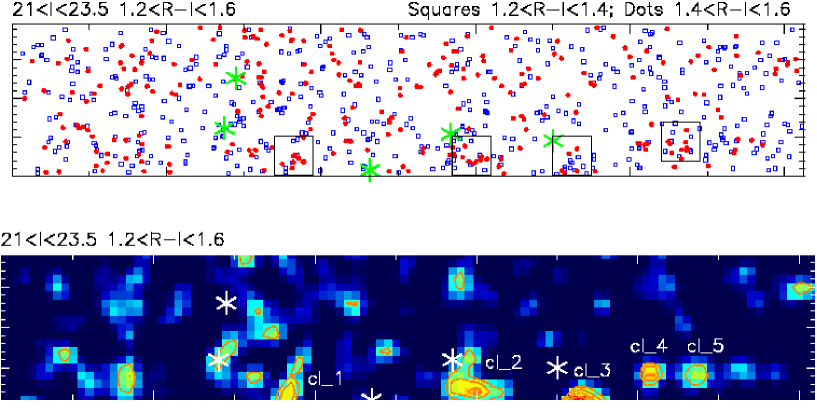
Figure 4: Top: Positions of the identified galaxy candidates ($21<I<23.5$) at $z\sim 1.1$ in the whole survey area ($48^{\prime}\times 9^{\prime}$). The position of each QSO is shown by asterisks. Dots and Boxes indicate galaxies with 1.4$<$R$-$I$<$1.6, and 1.2$<$R$-$I$<$1.4, respectively. Inset boxes indicate areas that are used for the analysis in Fig. 5. Bottom: Smoothed density map of the red galaxies with $21<I<23.5$ and $1.2<R-I<1.6$. The figure illustrates the amplitude of the density contrast in units of its rms value $\sigma$, and the plotted contours indicate the $2\sigma$, $3\sigma$, $4\sigma$ levels.

References

- Bertin & Arnouts (1996) Bertin, E., & Arnouts, S. 1996, A&AS, 117, 393
- Barrow, Bhavsar, & Sonoda (1984) Barrow J. D., Bhavsar,S. P., & Sonoda, D. H. 1984, MNRAS, 283, 1361
- Bower, Kodama, & Terlevich (1998) Bower, R. G., Kodama, T., & Terlevich, A. 1998, MNRAS, 299, 1193
- Boyle & Couch (1993) Boyle, B. J. & Couch W. J. 1993, MNRAS,264, 604
- Colles (1989) Colles, M. 1989, MNRAS, 237, 799
- Connolly et al. (1996) Connolly, A. J., Szalay, A. S., Koo, D., Romer, A. K., Holden, B., Nichol, R. C., & Miyaji, T. 1996, ApJ, 473, L67
- Crampton et al. (1988) Crampton, D., Cowley, A.P., Schmidtke, P.C., Janson, T., & Durrell, P. 1988, AJ, 96, 816
- Crampton et al. (1989) Crampton, D., Cowley, A.P., & Hartwick, F.D.A. 1989, ApJ, 345, 59
- Davis & Geller (1976) Davis, M., & Geller, M. J. 1976, ApJ, 208, 13
- de Lapparent, Geller, & Huchra (1986) de Lapparent, V., Geller, M. J., & Huchra, J. P. 1986, ApJ, 202, L1
- De Propris et al. (1999) De Propris, R., Stanford, S. A., Eisenhardt, P. R., Dickinson, M., & Elston, M. 1999, AJ, 118, 719
- Ellingson & Yee (1994) Ellingson, E., & Yee, H. K. C. 1994, ApJS, 92, 33
- Ford, Ciardullo, & Harms (1983) Ford, H., Ciardullo, R., & Harms, R. 1983, ApJ, 266, 451
- Graham, Clowes, & Campusano (1995) Graham, M. J., Clowes, G. C., & Campusano, L. E. 1995, MNRAS, 275, 790
- Groth & Peebles (1977) Groth, E. J., & Peebles, P. J. E. 1977, ApJ, 217, 385
- Hill & Lilly (1991) Hill, G. J., & Lilly, S. J.1991, ApJ, 367, 1
- Hutchings et al. (1993) Hutchings, J. B., Crampton, D., & Persram, D. 1993, AJ, 106, 1324
- Hutchings et al. (1995) Hutchings, J. B., Crampton, D., & Johnson, A. 1995, AJ, 109, 73
- Jaaniste et al. (1998) Jaaniste, J., Tago, E., Einasto, M., Einasto, J., Andernach H., & Müller, V. 1998, A&A, 336, 35
- Kajisawa et al. (2000a) Kajisawa, M., Yamada, T., Tanaka, I. et al. 2000a, PASJ, 52, 53
- Kajisawa et al. (2000b) Kajisawa, M., Yamada, T., Tanaka, I. et al. 2000b, PASJ, 52, 61
- Kodama & Arimoto (1997) Kodama, T., & Arimoto, N. 1997, A&A, 320, 41
- Komberg, Kravtsov, & Lukash (1996) Komberg, B. V., Kravtsov, A. V., & Lukash, V. N. 1996, MNRAS, 282, 713
- Landy & Szalay (1993) Landy, S. D., & Szalay, A. S. 1993, ApJ, 412, 64
- Le Fèvre et al. (1994) Le Fèvre, O., Crampton, D., Hammer, F., Lilly, S. J., & Tresse, L. 1994, ApJ, 423, L89
- Lilly et al. (1995) Lilly S. J., Tresse, L., Hammer, F., Crampton, D., & Le Fèvre, O. 1995, ApJ, 455, 108
- Lilly et al. (1998) Lilly S. J. et al. 1998, ApJ, 500, 75
- Longo (1991) Longo M. J. 1991, ApJ, 372, L59
- Lubin et al. (2000) Lubin, L. M., Brunner, R., Metzger, M. R., Postman, M., & Oke, J. B. 2000, ApJ, 531, L5
- Lumsden et al. (1997) Lumsden, S. L., Collins, C. A., Nichol, R. C., Eke, V. R., & Guzzo, L. 1997, MNRAS, 290, 119
- Oort, Arp, & de Riter (1981) Oort, J. H., Arp, H., & de Riter, H. 1981, A&A, 95, 7
- Postman & Geller (1984) Postman, M. & Geller, M. J. 1984, ApJ, 281, 95
- Postman et al. (1996) Postman, M., Lubin, L. M., Gunn, J. E., Oke, J. B., Hoessel, J. G., Schneider, D. P., & Christensen, J. A. 1996, AJ, 111, 615
- Postman et al. (1998) Postman, M., Lauer, T. R., Szapudi, I., & Oegerle, W. 1998, ApJ, 506, 33
- Ramella, Geller, & Huchra (1989) Ramella, M., Geller, M. J., & Huchra, J. P. 1989, ApJ, 344, 57
- Rosati et al. (1999) Rosati, P., Stanford, S. A., Eisenhardt, P. R., Elston, R., Spinrad, H., Stern, D., & Dey, A. 1999, AJ, 118, 76
- Sánchez & González-Serrano (1999) Sánchez, S. F. & González-Serrano, J. I. 1999, A&A, 352, 383
- Sandage (1988) Sandage, A. 1988, ARA&A, 26, 561
- Stanford, Eisenhardt, & Dickinson (1998) Stanford, S. A., Eisenhardt, P. R., & Dickinson, M. 1998, ApJ, 492, 461
- Schechter (1976) Schechter, P. 1976, ApJ, 203, 297
- Tanaka (2000) Tanaka, I., 2000, Doctoral thesis, Tohoku University
- Tanaka et al. (2000) Tanaka, I., Yamada, T., Aragón-Salamanca, A., Kodama, T., Miyaji, T., Ohta, K., & Arimoto, N. 2000, ApJ, 528, 123
- Teplitz, McLean, & Malkan (1999) Teplitz, H. I., McLean, I. S., & Malkan, M. A. 1999, ApJ, 520, 469
- Trasarti-Battistoni et al. (1997) Trasarti-Battistoni, R., Invernizzi, G., & Bonometto, S. A. 1997, ApJ, 475, 1
- Woods & Fahlman (1997) Woods, D. & Fahlman, G. G. ApJ, 1997, 490, 11
- Yamada et al. (1997) Yamada, T., Tanaka, I., Aragón-Salamanca, A., Kodama, T., Ohta, K., & Arimoto, N. 1997, ApJ, 487, L125
- Yee & Green (1984) Yee, H. K. C., & Green R. F. 1984, ApJS, 54, 495
- Yee (1990) Yee, H. K. C. 1990, in Evolution of Galaxies and Galaxy Clusters Associated with Quasars, Proceedings of the Edwin Hubble Centenial Symposium, Berkeley, p322
- Waldram et al. (1996) Waldram, E. M., Yates, J. A., Riley, J. M.,& Warner, P. J. 1996, MNRAS, 282, 779
- West (1991) West, M. J. 1991, ApJ, 379, 19
- Zabludoff & Mulchaey (1998) Zabludoff, A. I. & Mulchaey, J. S. 1998, ApJ, 496, 39