The Effects of Rotation on the Evolution of Rising Omega-loops in a Stratified Model Convection Zone

Abstract

We present three-dimensional MHD simulations of buoyant magnetic flux tubes that rise through a stratified model convection zone in the presence of solar rotation. The equations of MHD are solved in the anelastic approximation, and the results are used to determine the effects of solar rotation on the dynamic evolution an $\Omega$-loop. We find that the Coriolis force significantly suppresses the degree of fragmentation at the apex of the loop during its ascent toward the photosphere. If the initial axial field strength of the tube is reduced, then, in the absence of forces due to convective motions, the degree of apex fragmentation is also reduced. We show that the Coriolis force slows the rise of the tube, and induces a retrograde flow in both the magnetized and unmagnetized plasma of an emerging active region. Observationally, we predict that this flow will appear to originate at the leading polarity, and will terminate at the trailing polarity.

1 Introduction

Active regions represent the largest observable concentrations of magnetic flux on the Sun. The magnetic field within active regions exhibits a bipolar structure, which suggests that they are the tops of large $\Omega$-shaped loops which have risen through the convection zone and have emerged through the photosphere. On average, active region bipoles are oriented nearly parallel to the East-West direction (Hale’s Polarity Law). This suggests that the subsurface field geometry is approximately toroidal. Since active regions appear to be the tops of large, rising $\Omega$-loops, and since Hale’s law persists for years in a given solar cycle, we can infer that the toroidal flux must exist well below the solar surface, and that the magnetic flux must reside in a region where it is relatively free from disruption by buoyant instabilities or convective motions (Spruit & van Ballegooijen, 1982; van Ballegooijen, 1982; Ferriz-Mas & Schüssler, 1993, 1995). However, if the magnetic flux is embedded in the radiative zone (well below the convective zone) it would be so stable that it could not emerge through the surface on the time scale of a solar cycle (Parker, 1979; van Ballegooijen, 1982). This implies that the toroidal field likely resides in the “convective overshoot region” — a thin, slightly convectively stable layer located at the interface of the radiative and convective zones. This layer also appears to coincide with the “tachocline” (Kosovichev, 1996; Corbard et al., 1999), where the solid body rotational behavior of the radiative interior transitions into the differential rotation behavior observed in the convection zone. Thus, the toroidal field seems to be generated and stored in the overshoot layer. (Gilman, Morrow, & DeLuca, 1989; DeLuca & Gilman, 1991; Parker, 1993; MacGregor & Charbonneau, 1997; Durney, 1997; Dikpati & Charbonneau, 1999).

We now have a basic picture of how active regions might form: A portion of the toroidal flux layer eventually succumbs to one of several possible instabilities (eg. Caligari et al. 1995; Fan & Fisher 1996; Fan 2000; Wissink et al. 2000b), and forms a magnetically buoyant tube that begins to rise through the convection zone toward the photosphere. The top of the emerging flux loop is then observed at the photosphere as a bipolar magnetic region. The simplest way to model this picture is with the “thin flux tube” approximation (see Defouw 1976; Roberts & Webb 1978; Spruit 1981). In this simple model, it is assumed that magnetic flux tubes move through a field-free plasma, that the cross-section of the tube is much smaller than all other relevant length scales of the problem, and that pressure balance is always maintained across the tube. Given these assumptions, one can derive an equation of motion for a one-dimensional tube moving through a three dimensional medium. This model has had great success in explaining many of the observed properties of active regions, including (but not limited to) the variation and scatter of active region tilt as a function of solar latitude (D’Silva & Howard, 1993; D’Silva & Choudhuri, 1993; Fan et al., 1993; Caligari et al., 1995; Fisher et al., 1995; Longcope & Fisher, 1996; Fan & Fisher, 1996), the asymmetries in the orientation of active regions just after emergence (van Driel-Gesztelyi & Petrovay, 1990; Moreno-Insertis et al., 1994), and the latitudinal variation and fluctuations of field line twist from active region to active region (Longcope et al., 1998).

However, from the start, the thin flux tube approximation assumes that the magnetic field will retain its “tube-like” identity; that is, it will not fragment or disperse as it evolves. This assumption is called into question by recent two-dimensional MHD simulations which show that unless flux tubes possess a critical amount of initial field line twist along the tube — and observations of emerging active regions suggest that many do not (Pevtsov et al., 1995; Longcope et al., 1998, 1999) — the tubes will fragment (break apart) before they are able to emerge through the surface (Linton et al., 1996; Moreno-Insertis & Emonet, 1996; Emonet & Moreno-Insertis, 1998; Fan et al., 1998). Recently, Abbett et al. (2000) used three-dimensional MHD simulations to demonstrate that the degree of cohesion at the apex of an emerging $\Omega$-loop depends strongly on the three-dimensional geometry of the loop. If the curvature of the $\Omega$-loop at its apex is relatively large (ie. if the loop is tall and narrow), then the apex will emerge through the photosphere more cohesively than if the curvature is small (ie. if the $\Omega$-loop is short and wide). Dorch & Nordlund (1998) and Dorch et al. (1999) also performed detailed three-dimensional MHD simulations of buoyant magnetic flux tubes. All of these 3-D studies still require a significant amount of initial field line twist in order to suppress the eventual fragmentation of the tube near the loop apex. Is there a way out this quandary which Abbett et al. (2000) refer to as “Longcope’s paradox”?

In this paper, we investigate how solar rotation affects the dynamic evolution of buoyant magnetic flux tubes. We find that the Coriolis force plays a dynamically important role during the tube’s ascent, and acts to maintain the tube’s cohesion even in the absence of initial field line twist, possibly resolving Longcope’s paradox. In Section 2 we briefly describe our computational methodology, discuss how we include the Coriolis force in our computational model, and define the relevant physical parameters of our problem. In Section 3 we analyze the results of our simulations, and develop a very simple model that effectively characterizes the simulation results pertaining to flux tube cohesion. In this section we also comment on possible observational consequences of the simulations. Finally, we present our summary and conclusions in Section 4.

2 Method

We use the methods described in Abbett et al. (2000) and Fan et al. (1999) to solve the three-dimensional equations of MHD in the anelastic approximation (Ogura & Phillips, 1962; Gough, 1969; Lantz & Fan, 1999). The anelastic equations result from an expansion of the equations of compressible MHD about a zeroth order reference state (which we take to be a field-free, adiabatically stratified polytrope of index $m=1.5$). In this approximation, the higher order time derivative of the perturbed density is neglected, effectively filtering out fast-moving acoustic waves. This is computationally advantageous, as it allows for much larger timesteps than would be possible in a fully compressible calculation. This approximation is valid in sub-surface regions where the acoustic Mach number is small ($M\equiv v/c_{\mathrm{s}}\ll 1$), and where the local sound speed ($c_{\mathrm{s}}$) greatly exceeds the Alfvén speed ($v_{A}$) of the plasma (Glatzmeier, 1984). A detailed theoretical discussion of the anelastic formulation can be found in Lantz & Fan 1999 (and references therein).

The anelastic equations in a non-rotating reference frame are given by equations [1]-[7] in Abbett et al. (2000) (hereafter AFF). To consider the effects of solar rotation, we adjust the anelastic momentum equation to include non-inertial terms (we note, here, that due to a typesetting error in the final version of AFF, a cross-product symbol was omitted in the Lorentz force term of equation [2]). To consider the effects of solar rotation, we adjust the anelastic momentum equation to include non-inertial terms. In this study, we neglect centrifugal effects and concentrate only on the effects of the Coriolis force due to solid-body rotation. In this approximation, the anelastic momentum equation (in the rotating reference frame) becomes:

$$\rho_{0}\left(\frac{\partial\mathbf{v}}{\partial{t}}+\mathbf{v}\cdot\mbox{\boldmath$\nabla$\unboldmath}\mathbf{v}\right)=-\mbox{\boldmath$\nabla$\unboldmath}p_{1}+\rho_{1}\mathbf{g}-2\rho_{0}\left(\mbox{\boldmath$\Omega$\unboldmath}\times\mathbf{v}\right)+\frac{1}{4\pi}\left(\mbox{\boldmath$\nabla$\unboldmath}\times\mathbf{B}\right)\times\mathbf{B}+\mbox{\boldmath$\nabla$\unboldmath}\cdot\mathbf{\Pi}\,.$$ (1)

Here, $\rho_{0}$ refers to the density stratification of the zeroth order reference state, while $\rho_{1}$, $p_{1}$, $\mathbf{v}$, and $\mathbf{B}$ represent the density, pressure, velocity and magnetic field perturbations. The viscous stress tensor is given by $\Pi_{ij}\equiv\mu(\partial v_{i}/\partial x_{j}+\partial v_{j}/\partial x_{i}-2/3(\mbox{\boldmath$\nabla$\unboldmath}\cdot\mathbf{v})\delta_{ij})$, where $\mu$ is the coefficient of viscosity and $\delta_{ij}$ is the Kronecker delta function. $\,\Omega$ denotes the angular velocity about the Sun’s axis of rotation. Both the acceleration due to gravity, ${\rm g}\mbox{\unboldmath$\,=-$g}\,\hat{z}$, and the coefficient of viscosity are assumed constant in our calculations.

We solve the non-dimensional form of the anelastic equations in the modified, local f-plane approximation of Brummell et al. (1996). This approach is similar to the standard f-plane approximation of geophysical fluid dynamics (Pedlosky, 1987), except that the transverse components of the Coriolis force within the rectangular domain are retained. Since $\Omega$ is assumed constant throughout the Cartesian box (positioned at a given latitude), we can apply simple, periodic boundary conditions in the horizontal directions, and stress-free, non-penetrating conditions at the upper and lower boundaries. Further simplification is possible by noting that the momentum density (in the anelastic approximation) and magnetic field vectors are both divergence-free. This allows us to define scalar potentials such that $\mathbf{B}\equiv\mbox{\boldmath$\nabla$\unboldmath}\times\mbox{\boldmath$\nabla$\unboldmath}\times\mathcal{B}\!\!$ $\hat{z}$ $+\,\mbox{\boldmath$\nabla$\unboldmath}\times\mathcal{J}\!\!$ $\hat{z}$ and
$\rho_{0}\mathbf{v}\equiv\mbox{\boldmath$\nabla$\unboldmath}\times\mbox{\boldmath$\nabla$\unboldmath}\times\mathcal{W}\!\!$ $\hat{z}$ $+\,\mbox{\boldmath$\nabla$\unboldmath}\times\mathcal{Z}\!\!$ $\hat{z}$ . Along with the other dependent variables of the system, these potentials are decomposed spectrally in the horizontal directions:

$$\mathcal{Q}=\sum_{\rm{mn}}\widetilde{\mathcal{Q}}_{\rm{mn}}(z)e^{2\pi i\left(f_{\rm{m}}x\,+\,g_{\rm{n}}y\right)}\,.$$ (2)

Here, $\mathcal{Q}$ and $\widetilde{\mathcal{Q}}_{\rm{mn}}$ refer to a given dependent variable or scalar potential and its associated Fourier coefficient. $f_{\rm{m}}$ and $g_{\rm{n}}$ are defined as ${\rm{m}}/\mathcal{L}_{x}$ and ${\rm{n}}/\mathcal{L}_{y}$ respectively, where $\mathcal{L}_{x}$ and $\mathcal{L}_{y}$ denote the size of the domain in the $\hat{x}$ and $\hat{y}$ directions. The integers ${\rm{m}}$ and ${\rm{n}}$ range from $-{\rm{N}}_{x}/2+1$ to ${\rm{N}}_{x}/2$ and $-{\rm{N}}_{y}/2+1$ to ${\rm{N}}_{y}/2$. ${\rm{N}}_{x}$ and ${\rm{N}}_{y}$ refer to the number of zones in the $\hat{x}$ and $\hat{y}$ directions. The Fourier coefficients are then discretized with respect to the vertical direction (defined to be parallel to $\mathbf{g}$), and vertical derivatives are approximated by fourth-order, centered finite differences. Using the semi-implicit method of operator splitting, we apply the second-order Adams-Bashforth scheme to the advection terms, and the second-order Crank-Nicholson scheme to the diffusion terms (see Press et al. 1986 for a description of these methods).

A detailed, in-depth description of the techniques we employ to obtain a solution to the anelastic equations in a non-rotating reference frame can be found in Appendix A of Fan et al. (1999) (hereafter FZLF). Only minor modifications are necessary to extend that formalism to apply in the case of a rotating reference frame in the modified f-plane approximation. The equation for the time evolution of $\widetilde{\mathcal{Z}}_{\rm{mn}}$, the Fourier coefficients of the spectral decomposition of $\mathcal{Z}$, is obtained by evaluating the $\hat{z}$-component of the curl of the momentum equation. Thus, the addition of the Coriolis term to equation (1) results in an additional non-inertial term to equation (A16) of FZLF:

$$\left(\frac{\partial\widetilde{\mathcal{Z}}_{\rm{mn}}}{\partial t}\right)_{\rm{cor}}=\;2\Omega_{z}\frac{\partial\widetilde{\mathcal{W}}_{\rm{mn}}}{\partial z}+4\pi i\widetilde{\mathcal{W}}_{\rm{mn}}\left(f_{\rm{m}}\Omega_{x}+g_{\rm{n}}\Omega_{y}\right)\,.$$ (3)

Here, the $\Omega_{i}$’s represent the Cartesian components of the angular velocity vector, and $\widetilde{\mathcal{W}}_{\rm{mn}}$ denotes the Fourier coefficients of the scalar potential $\mathcal{W}$. Equation (A18) of FZLF results from taking the $\hat{x}$ and $\hat{y}$ components of the curl of the momentum equation as it appears in equation (A4). Thus, we must add another term to equation (A18) to reflect the addition of the Coriolis force to equation (1):

$$\left(\frac{\partial\widetilde{\psi}_{\rm{mn}}}{\partial t}\right)_{\rm{cor}}=\;-2\Omega_{z}\frac{\partial}{\partial z}\left(\frac{\widetilde{\mathcal{Z}}_{\rm{mn}}}{\rho_{0}}\right)+\frac{4\pi i}{\rho_{0}h_{0}}\widetilde{\mathcal{W}}_{\rm{mn}}\left(f_{\rm{m}}\Omega_{y}-g_{\rm{n}}\Omega_{x}\right)-\frac{4\pi i}{\rho_{0}}\widetilde{\mathcal{Z}}_{\rm{mn}}\left(f_{\rm{m}}\Omega_{x}+g_{\rm{n}}\Omega_{y}\right)\,.$$ (4)

In the above equation, $\widetilde{\psi}_{\rm{mn}}\equiv-i(2\pi)^{-1}(f_{\rm{m}}^{2}+g_{\rm{n}}^{2})^{-1}(f_{\rm{m}}\widetilde{\omega}_{y\rm{mn}}-g_{\rm{n}}\widetilde{\omega}_{x\rm{mn}})$ is the scalar variable that corresponds to $\widetilde{\Omega}_{\rm{mn}}$ in equation (A18) of FZLF (we change notation so as to avoid confusion with the components of the angular velocity vector); $\,\widetilde{\omega}_{x\rm{mn}}$ and $\widetilde{\omega}_{y\rm{mn}}$ are the Fourier coefficients of the $\hat{x}$ and $\hat{y}$ components of the vorticity; and $h_{0}\equiv-\rho_{0}(\partial\rho_{0}/\partial z)^{-1}$ is the density scale height. The last necessary modification is to equations (A23) and (A24) of FZLF where we add the contribution from the horizontal average of the Coriolis term in the momentum equation: $(\partial(\rho_{0}\overline{v}_{x})/\partial t)_{\rm{cor}}=2\rho_{0}\Omega_{z}\overline{v}_{y}$ and $(\partial(\rho_{0}\overline{v}_{y})/\partial t)_{\rm{cor}}=-2\rho_{0}\Omega_{z}\overline{v}_{x}$. Here, $\overline{v}_{x}$ and $\overline{v}_{y}$ denote the horizontal averages of the $\hat{x}$ and $\hat{y}$ components of the velocity (note that $\overline{v}_{z}$ is zero).

We now turn our attention to the non-dimensional formulation of the anelastic equations as implemented in the code. As was described in AFF, many of the dimension-less physical variables and fundamental physical parameters are expressed in terms of the magnetic field strength along the axis of the initial flux tube, $B_{0}$. With the addition of the Coriolis force to the momentum equation, we introduce another fundamental dimension-less quantity, $R_{b}\equiv v_{\!A}/(2\Omega H_{r})\equiv 1/(2\Omega^{\prime})$, which we refer to as the “magnetic Rossby number” (a quantity also discussed by Schüssler & Solanki 1992). Here, $\Omega^{\prime}$ is defined as the non-dimensional rotation rate given in terms of the ratio of the characteristic velocity scale to the characteristic length scale of our problem; namely, the pressure scale height at the base of the computational domain ($H_{r}$), and the Alfvén speed along the axis of the initial tube ($v_{\!A}\equiv B_{0}/(2\sqrt{\pi\rho_{r}})$, where the characteristic density, $\rho_{r}$, is taken to be the density at the lower boundary). The magnetic Rossby number is a measure of the relative importance of the Coriolis force on the dynamic evolution of our buoyant magnetic flux tube. Rotational effects become important when $R_{b}<1$, and are less significant when $R_{b}>1$. We therefore wish to investigate three representative cases: $R_{b}=1/2$, $R_{b}=1$, and $R_{b}=2$. Of course, the solar rotation rate is not a free parameter — estimates of $\Omega$ in different parts of the convection zone can be obtained from helioseismologic measurements. Thus, varying the magnetic Rossby number to investigate the effect of solar rotation on a buoyant magnetic flux tube amounts to varying the initial axial field strength of the tube.

The specification of $B_{0}$ impacts the scaling of two of the non-dimensional diffusive parameters: the Reynolds number ($R_{e}\equiv[\rho][l][v]\mu^{-1}$), and the magnetic Reynolds number ($R_{m}\equiv[l][v]\eta^{-1}$). Again, the characteristic length, velocity, and density scales ($[l]$, $[v]$, and $[\rho]$) are given in terms of $H_{r}$, $v_{\!A}$, and $\rho_{r}$ respectively. For this study, we hold the coefficients of viscosity and magnetic diffusion ($\mu$ and $\eta$ respectively) constant between runs (where possible), and vary $B_{0}$ such that we obtain our three representative values of the magnetic Rossby number. In this manner, we focus our attention on the effects of solar rotation on the dynamic evolution of a rising $\Omega$-loop. We note however, that as $B_{0}$ becomes large, it is increasingly difficult to hold the coefficient of viscosity constant for a given grid resolution. This is because as the Reynolds number increases, features develop at the forefront of the rising tube and in the trailing eddies that are on the order of a few grid zones in size. If this occurs, the code becomes unstable, and the grid resolution must be increased to alleviate the problem. Table 1 lists the values of the relevant physical parameters for each of seven simulations. For the cases where $B_{0}\sim 10^{5}$G, values of $\mu$ and $\eta$ were increased to avoid instabilities. We otherwise would have to double the grid resolution in the tube cross-section to take full advantage of the FFT algorithms employed in the code, and such a large increase is unnecessary for the purposes of this study.

Our labeling convention (see column one of Table 1) consists of four letters which signify both the strength of $B_{0}$, and the latitude of the computational box. For example, LFHL refers to the run which has an initial magnetic flux tube with a relatively Low axial Field strength positioned at a High Latitude, while HFLL refers to the run with an initial tube of relatively High axial Field strength positioned at Low Latitude — and so on. Run SS0 refers to the simulation where solar rotation was neglected (this notation was chosen in order to be consistent with the naming convention of AFF). In each case, we begin with a static, horizontal, cylindrical magnetic flux tube positioned near the bottom of a simulation box that spans 5.147 pressure scale heights vertically. The initial field configuration is given by $\mathbf{B}=B_{x}(r)\mbox{\boldmath$\hat{x}$\unboldmath}$, where $B_{x}(r)\equiv B_{0}e^{-r^{2}/a^{2}}$ and $r$ is the radial distance to the central axis in the tube’s cross-section. The size of the initial tube, $a$, is taken to be $0.1H_{r}$ in each of the simulations. We choose not to include any initial field line twist about the central axis of the tube, since we wish to determine what role the Coriolis force alone plays in the overall fragmentation of the tube as it rises toward the photosphere. As was done in AFF, we apply an artificial entropy perturbation to the midsection of the tube at time $t=0$. This causes the tube to rise as an $\Omega$-loop without having to take the computationally expensive step of evolving each case self-consistently from a state of initial force balance (as was done in Caligari et al. 1995; Fan & Fisher 1996; Fan 2000).

3 Results

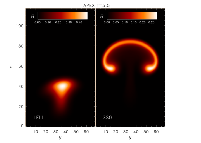
Figure 1: Apex cross-sections of $|\mathbf{B}|$ for a simulation with $R_{b}=0.5$ at $15^{\circ}$ latitude (left frame, run LFLL), and a simulation neglecting solar rotation (right frame; labeled run SS0 to be consistent with the naming convention of AFF). $|\mathbf{B}|$ is given in terms of the field strength along the axis of the initial tube, and $t$ is given in units of the ratio of the pressure scale height at the base of the domain to the Alfvén speed along the axis of the initial tube. The coordinate axes are given in terms of computational zones, though only a portion of the domain is shown.

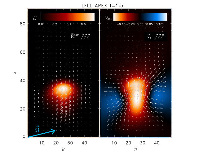
Figure 3: Apex cross-sections of $|\mathbf{B}|$ along with the transverse Coriolis force (left frame), and the corresponding velocity field (right frame) for run LFLL ($R_{b}=0.5$ at $15^{\circ}$ latitude) at $t=1.5$. Quantities are given in naturalized units (see text for details). In the right frame, axial flows depicted in red indicate velocities receding from the viewer, while blue colors indicate flow moving toward the viewer. Here, max$|\mathbf{v}_{x}|/$max$|\mathbf{v}_{T}|\approx 1.5$; that is, the axial flows are stronger than the transverse flows. The angular velocity vector is displayed in the lower left-hand corner of the left frame, and applies to the entire figure.

Each simulation begins with an untwisted cylindrical magnetic flux tube embedded near the base of our model convection zone. An entropy perturbation is applied to the flux tube such that in the absence of rotation, the tube will rise as an $\Omega$-loop, and the apex will approach the photospheric boundary in a highly “fragmented” state. That is, a majority of the magnetic flux will be concentrated away from the tube’s central axis along vortex pairs that are shed during the tube’s ascent. Following AFF, we consider a section of the $\Omega$-loop to be fragmented if the ratio of the magnetic field weighted second moments of position along the Frenet binormal and normal directions of the tube exceed $1.5$ (see Section 3 of AFF for details on how tube fragmentation is determined, and see Figures 1 and 3 in AFF for visual examples of a fragmented and non-fragmented $\Omega$-loop). We expect that solar rotation will play a dynamically important role during the tube’s ascent, since the loop’s rise time is on the order of a rotation period for reasonable initial field strengths ($3\times 10^{4}$G $\lesssim B_{0}\lesssim 1\times 10^{5}$G, see Fisher et al. 2000).

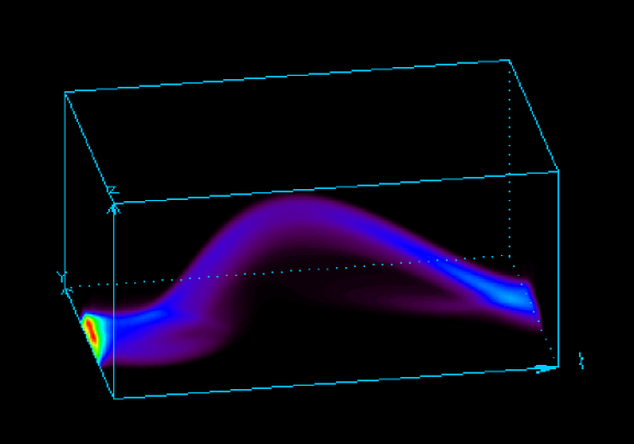
Figure 2: A volume rendering of $|\mathbf{B}|$ for the $\Omega$-loop of run HFLL at $t=8.53$. The entire rectangular computational domain is shown.

We find that the impact of the Coriolis force on a rising flux tube is dramatic, as demonstrated in Figure 1. In this figure, we compare the magnetic field strength in the apex cross-section of two $\Omega$-loops: one which rises at $15^{\circ}$ latitude in the presence of solar rotation ($\Omega\sim 13.9^{\circ}$/day) with an initial axial field strength of $B_{0}=2.67\times 10^{4}\,$G (corresponding to $R_{b}=0.5$), and an identical loop which rises in the absence of rotation. Two effects are immediately apparent. First, the $\Omega$-loop that rises through the rotating atmosphere has yet to attain the height of the loop that rises through the non-rotating atmosphere; and second, the loop subjected to the effects of the Coriolis force retains its cohesion, and does not fragment. Figure 2 is a volume rendering of a rising magnetic flux tube in a run where $R_{b}=2$ and $B_{0}=1.0\times 10^{5}\,$G. The coordinate axes are chosen such that $\hat{y}$ points northward, and $\hat{z}$ points radially outward. Again, we see that the tube retains its cohesion during its ascent. Figure 2 also demonstrates that in the presence of rotation, the $\Omega$-loop is somewhat asymmetric about the apex. That is, the trailing portion of the loop forms a steeper angle with respect to the $\hat{x}$ direction than the leading side of the loop.

A qualitative understanding of these effects can be obtained by examining Figure 3, which shows $|\mathbf{B}|$, the transverse components of the Coriolis force, and the flow field in the apex cross-section during the initial stages of run LFLL (an earlier snapshot of the same run that is displayed in the left frame of Figure 1). In this plot (and all others, unless otherwise stated) the physical quantities are displayed in naturalized units: the magnetic field strength is given in terms of the strength of the field along the axis of tube at $t=0$ ($B_{0}$), the velocities are given in terms of the Alfvén speed along the axis of the initial tube ($v_{\!A}$), and the unit of time is the ratio of the pressure scale height at the base of the computational domain to the characteristic velocity, $H_{r}/v_{\!A}$. For run LFLL, shown in Figure 3, $B_{0}=2.67\times 10^{4}\,$G, $v_{\!A}=1.68\times 10^{4}$ cm s$\!\,{}^{-1}$ (for $\rho_{r}=0.2$ g cm$\!\,{}^{-3}$), and $t=1.5$ corresponds to $6.18$ days. The axes in the figure are given in terms of computational zones; in this case, each individual zone is $0.017H_{r}$, or approximately $1$ Mm.

In the right-hand frame of Figure 3 we see that a strong, retrograde axial flow has developed as a result of the Coriolis force acting on rising material within the buoyant loop. This is in sharp contrast to the simulations in AFF, where solar rotation is neglected and the initial flux tube has little or no field line twist. In these cases, the strong axial flow is absent, and counter-rotating vortex pairs can quickly form on either side of the tube’s central axis (see also Wissink et al. 2000a; Dorch & Nordlund 1998). As was shown in AFF and Longcope et al. (1996), the non-vertical component of the hydrodynamic “lift” force per unit volume generated by flows in the vortex tubes acts to push them apart, ultimately resulting in fragmentation near the apex of the $\Omega$-loop. However, in the presence of rotation, we find that the circulation (and thus the degree of fragmentation of the loop) is substantially reduced. Roughly speaking, this follows from the fact that the Coriolis force can do no work (it always acts in a direction perpendicular to the flow); it simply redistributes kinetic energy between transverse and axial flows. The initial increase in the axial flow at the apex of the loop gives rise to a secondary effect: a transverse component of the Coriolis force normal to the angular velocity vector. At low latitudes, this component acts primarily in the $-$$\hat{z}$ direction, and opposes the buoyant rise of the loop; however, it also forces the top of the loop to drift northward over time.

In simulations where the effects of rotation are neglected, we find that material flows along the rising tube away from the apex. In the presence of rotation, this type of “draining” flow manifests itself as an asymmetry in the axial flow induced by the Coriolis force: the retrograde flow is stronger in the trailing side of the loop than it is in the leading side. As the Coriolis force acts upon these asymmetric axial flows, and as the buoyant, magnetized plasma attempts to preserve its angular momentum, the morphological asymmetry predicted by Moreno-Insertis et al. (1994) and apparent in Figure 2 quickly develops.

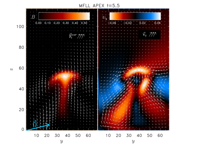
Figure 4: Same as Figure 3 for run MFLL ($R_{b}=1$ at $15^{\circ}$ latitude) at $t=5.5$ (the same time as displayed in Figure 1). Here, max$|\mathbf{v}_{x}|/$max$|\mathbf{v}_{T}|\approx 1.1$.

Figure 4 shows the transverse components of the Coriolis force, and the flow field in the apex cross-section of run MFLL at $t=5.5$ (the same time, in naturalized units, as the cross-sections of Figure 1). In this run, $R_{b}=1$, and the domain is again centered at $15^{\circ}$ latitude. This implies that $B_{0}=5.35\times 10^{4}\,$G, $v_{\!A}=3.37\times 10^{4}\,$cm s$\!\,{}^{-1}$, and the unit of time is 2.06 days ($t=5.5$ thus corresponds to $11.3$ days). In an earlier snapshot of run MFLL ($t=1.5$), the morphology and flow patterns are very similar to those shown for run LFLL in Figure 3. However, as the runs progress, differences in secondary and tertiary flows become more pronounced, and the loops begin to evolve in a dissimilar manner. This is evident when comparing the first frame of Figure 4 with the frames of Figure 1, which highlight the striking differences in morphology that ultimately develop between simulations with different values of the magnetic Rossby number. These figures show that as the initial axial magnetic field strength of the tube is increased, the tendency for the tube to fragment as it rises toward the photosphere is also increased.

3.1 An Approximate Model

To better understand the relationship between magnetic Rossby number, latitude of flux emergence, and loop fragmentation, we approximate the forcing terms of the momentum equation [equation (1)] by constant, order-of-magnitude estimates evaluated for our initial conditions, and valid for the initial stages of evolution. We then have a simplified expression for the velocity field that admits to an analytic solution:

$$\frac{d\mathbf{v}}{dt}=-2\left(\mbox{\boldmath$\Omega$\unboldmath}\times\mathbf{v}\right)+\mathbf{Q}\,.$$ (5)

It is important to recognize that this simple approximation will not capture the factor of two reduction in acceleration that occurs in the non-rotating case because of “added inertia” effects (see Longcope et al. 1996). Nevertheless, it does capture the essence of the dynamic effects introduced by the Coriolis force. Let $(q_{x},q_{y},q_{z})$ represent the Cartesian components of the constant driving term $\mathbf{Q}$, and let $\theta$ represent solar latitude. Then the general solution to the above equation is given by

$$v_{x}(t) = \frac{q_{x}}{2\Omega}\sin{2\Omega t}-v_{x}^{(P)}\cos{2\Omega t}+v_{x}^{(P)}$$ (6)

$$v_{y}(t) = \frac{q_{x}}{2\Omega}\sin{\theta}\cos{2\Omega t}+v_{x}^{(P)}\sin{\theta}\sin{2\Omega t}$$ (7)

$$\;\;\;\;\;\;\;\;+\;(q_{y}-2\Omega v_{x}^{(P)}\sin{\theta})t-\frac{q_{x}}{2\Omega}\sin{\theta}$$

$$v_{z}(t) = -\frac{q_{x}}{2\Omega}\cos{\theta}\cos{2\Omega t}-v_{x}^{(P)}\cos{\theta}\sin{2\Omega t}$$ (8)

$$\;\;\;\;\;\;\;\;+\;(q_{z}+2\Omega v_{x}^{(P)}\cos{\theta})t+\frac{q_{x}}{2\Omega}\cos{\theta}\,,$$

where

$$v_{x}^{(P)} = \frac{1}{2\Omega}(q_{y}\sin{\theta}-q_{z}\cos{\theta})\,.$$ (9)

The total circulation over a cross-sectional slice of the flux tube is given by $\Gamma=\int_{S}\,$$\omega$$\,\cdot\,\hat{\mathbf{n}}_{S}\,dS=\oint_{C}\mathbf{v}\cdot d$$\ell$ , where $C$ is the closed circuit bounding the cross-sectional surface $S$, $\hat{\mathbf{n}}_{S}$ is the outward normal to $S$, and $\omega$$=$$\nabla$$\times\mathbf{v}$ is the vorticity vector. As the tube begins to rise, oppositely directed circulation patterns form on either side of a line defined by the Frenet normal. The total circulation of these regions (at the loop apex) is given by $\Gamma=\oint_{C}\mathbf{v}\,\cdot d$$\ell$$\,\,\,\approx\,\int_{\ell_{a}}d\ell_{a}\,v_{z}\,\approx\,a\!<\!v_{z}\!>$, if we assume that the primary contribution to $\Gamma$ stems from $\mathbf{v}\cdot d$$\ell$  across the diameter of the tube, $a$. Since $v_{z}$ is roughly constant across the interior of the tube, we can approximate the circulation (and thus the forces acting to pull the tube apart) with our analytic solution for the velocity. Initially, the motion of the tube is determined by the buoyancy force, which acts in the $\hat{z}$ direction. Thus, we assume that $q_{x}$ and $q_{y}$ are zero, and express the circulation as:

$$\Gamma(t)=\frac{{av_{\!A}}^{\!2}}{2H_{r}}\left(t\sin^{2}\theta+\frac{\sin(2\Omega t)}{2\Omega}\cos^{2}\theta\right)\,.$$ (10)

We plot our simple approximation of $\Gamma(t)$ for four representative values of $R_{b}$ in Figure 5.

In order to compare our approximation with the MHD solution, we must first obtain $\Gamma(t)$ directly from the simulation data. To accomplish this, we follow the methodology described in Section 3 of AFF, and first calculate the path of the magnetic flux tube through the background plasma. The position of the loop (and its fragments, if applicable) is specified by the magnetic field weighted first moments of position along a series of two-dimensional slices that closely correspond to the tube’s cross-sectional plane. Once the path of the tube is determined (see Section 3 of AFF), we construct the Frenet basis vectors, and define two regions on either side of a line defined by the Frenet normal where the oppositely directed circulation patterns will develop. From the simulation results, we then compute the total circulation across each of these regions. Figure 6 shows $\Gamma(t)$ for each simulation. One can compare these results with the simple approximation shown in Figure 5. It is clear that the general pattern of time dependence of the circulation is successfully reproduced by our simple model, though there are significant differences in the details.

The oscillations in $\Gamma(t)$ are inertia waves (see Batchelor 1967) with a period of $t=2\pi R_{b}$ (here, $t$ is expressed in normalized units of $H_{r}/v_{\!A}$). Thus, the tendency for the loops to fragment is significantly reduced after the circulation begins to fall off at $t=\pi R_{b}/2$. The overall evolution of the loop depends strongly on the dynamics during the initial portion of its rise, since the early differences in secondary and tertiary flows induced by the Coriolis force have a significant impact on the eventual evolution of the tube. We find that if the tube is able to rise several of its diameters before $t$ reaches $\pi R_{b}/2$, then the resulting $\Omega$-loop will ascend toward the photosphere in a fragmented state — otherwise, the tube evolves cohesively.

We can infer from our approximate model that, on average, the rise speed of the tube slowly increases over time. This prediction is confirmed by the simulations, which (for sufficiently high choices of $R_{e}$ and $R_{m}$) show the initial slow, linear increase in the rise speed of the tube, modulated by inertial oscillations. This behavior persists in the simulations until $t$ becomes comparable to the diffusive timescale. If this occurs, magnetic diffusion begins to (artificially) reduce the buoyancy of the tube, eventually preventing it from approaching the upper boundary (this occurred in runs LFLL and LFHL after $t\approx 34.0$). Of course, this problem can be mitigated by reducing the coefficient of magnetic diffusivity in the simulations, but this requires a significant increase in grid resolution (to avoid numerical instabilities); and since our analysis concentrates on the early stages of loop evolution, such a computationally expensive step is unwarranted.

3.2 Comparison with Two-dimensional Models

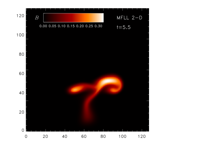
Figure 7: A cross-section of $|\mathbf{B}|$ at $t=5.5$ (in normalized units) for a 2-D run that begins with the initial magnetic flux tube of run MFLL.

To investigate the role that three-dimensional geometry plays in the tube’s evolution, we compare our runs with simulations of buoyant, axially symmetric magnetic flux tubes moving in two dimensions. Figure 7 shows the tube cross-section of a 2-D run whose parameters are that of the 3-D run MFLL shown in the first frame of Figure 4. This 2-D case can be thought of as an infinitely-long, buoyant, axially symmetric $\Omega$-loop of zero apex curvature. A comparison of the apex cross-section shown in Figure 4 with the cross-section of Figure 7 reveals that a 2-D geometric constraint imposed on the solution (even in the early stages of loop evolution) significantly alters the dynamic evolution of the tube. This suggests that in the presence of solar rotation, the geometry of the $\Omega$-loop still plays an important role in determining the morphology of the emerging magnetic field — a result consistent with the findings of AFF for similar runs where solar rotation was neglected.

In 2-D, the Coriolis force still acts to suppress the fragmentation of the tube. However, the hydrodynamic “lift” force that acts to fragment the tube is overestimated due to the tube’s effectively infinite axial length scale. It is the binormal component of this force that acts to pull the tube apart (see Longcope et al. 1996; Fan et al. 1998; AFF), thus the overall tendency for the tube to retain its cohesion during its ascent is reduced as compared to the 3-D cases. In addition, the amount that the tube is deflected toward the pole is significantly overestimated in a 2-D geometry. This is because in 3-D, the component of the Coriolis force that acts to push the tube poleward acts only on the portion of the $\Omega$-loop where there are strong, mainly axial flows (eg. near the apex). In general, our calculations support the conclusions of Wissink et al. (2000a) who used 2-D simulations to demonstrate that in the presence of the Coriolis force, flux tubes remained somewhat more cohesive during their ascent. We note, however, that in 3-D, this effect is more dramatic.

3.3 Morphology of the Emerging Magnetic Field

There are several reasons why we must be cautious when making predictions about the behavior of emerging magnetic flux based on data obtained from our simulations. First, the anelastic approximation becomes marginal as the flux tube approaches the photospheric boundary, where densities are lower, and the acoustic Mach number of the flow approaches unity. Second, we intended for these simulations to investigate the effects of the Coriolis force alone on the evolution of our $\Omega$-loop. Thus, we did not include any field line twist along our initial tube, nor did we consider the effects of a tube rising through a dynamically convecting background state. Third, our models do not account for radiative losses that occur at the surface. However, given these caveats, we feel that we can still make some general predictions regarding expected magnetic field and velocity flow patterns if the magnetic flux emerges through a relatively uncluttered region on the solar disk.

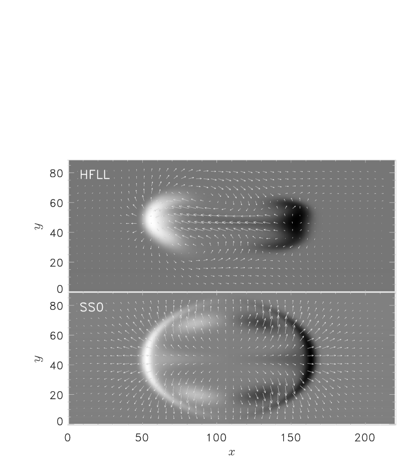
Figure 8: A grey-scale image of the radial magnetic field for a horizontal slice just below the apex of the $\Omega$-loops of the final timesteps of runs HFLL (top frame) and SS0 (bottom frame). The vector field represents the transverse ($x$-$y$) flow field. The $x$ and $y$ scales are given in terms of computational zones. The grid is uniform; each zone is roughly $1$ Mm in size. There is a very slight tilt of approximately $2.5$ degrees from horizontal between the center of the bipolar regions.

Figure 8 shows the radial component of the magnetic field along horizontal slices taken underneath the apex of the rising $\Omega$-loops of runs HFLL, and SS0. This figure emphasizes the differences in morphology of emerging magnetic field between a simulation that includes the effects of solar rotation (run HFLL), and one that does not (run SS0). In the figures, outwardly directed field is displayed in white, and inwardly directed field is displayed in black. Superimposed over the each grey-scale image is the transverse velocity field. One of the most striking effects of the Coriolis force is the strong flow that rapidly develops in both the magnetized and unmagnetized plasma directed from the leading toward the trailing polarity (the leading polarity moves in the direction of solar rotation as the loop continues to rise). This flow is simply the result of the Coriolis force acting on the rising fluid just below the apex of each loop. This “LTT” (Leading To Trailing polarity) flow is evident in all of our simulations except in cases where solar rotation is neglected.

The Coriolis force manifests itself in several other interesting ways. First, since the trailing edge of the loop emerges at a steeper angle with respect to the surface than the leading edge (an effect most pronounced in the runs where $R_{b}$ is small), the leading polarity becomes “spread-out” in the east-west direction (along $x$). Second, in the cases where $R_{b}$ is small, we observe that the leading polarity is positioned slightly closer to the equator than the trailing polarity — behavior that is roughly consistent with the “Joy’s Law” result from thin flux tube models (see D’Silva & Choudhuri 1993; Fan et al. 1994; Schüssler et al. 1994; Caligari et al. 1995; Fan & Fisher 1996; Fisher et al. 2000). Third, the north-south dispersion of the emerging flux is greatly reduced when solar rotation is included in the simulations. This reflects the increased cohesion of the flux rope during its ascent through our model convection zone.

4 Summary and Conclusions

AFF found that the degree of fragmentation of a rising $\Omega$-loop depends upon the 3-D geometry of the loop — the greater the apex curvature, the lesser the degree of fragmentation for a fixed amount of initial field-line twist. We are now able to extend this analysis to a rotating model convection zone, and investigate how the degree of apex fragmentation depends on the axial field strength of the initial magnetic flux tube. Assuming a given rotation rate, we find that:

1. A magnetic flux tube that rises buoyantly toward the photosphere in a rotating convection zone rises more slowly, and is better able to retain its cohesion than an identical flux tube that rises through a non-rotating convection zone — even in the absence of initial field line twist. If the tube is sufficiently buoyant so that it is able to rise a distance of several tube diameters before $t=\pi/4\Omega$ (where $\Omega$ is an estimate of the relevant solar rotation rate at a given latitude), then the tube will fragment during its rise toward the photosphere.

2. In the absence of forces due to convective motions, the stronger the initial axial field strength of the tube, the more fragmentation occurs as the tube rises.

3. An approximate model is able to predict the initial evolution of the circulation, and hence can effectively characterize the formation and subsequent interaction of the oppositely-directed vortex pairs of a fragmented $\Omega$-loop.

4. One must be careful not to over-interpret results from two-dimensional simulations of buoyant magnetic flux tubes. In a two-dimensional geometry, hydrodynamic forces due to vortex interaction are overestimated. The amount of poleward deflection due to the Coriolis force is also overestimated.

5. If magnetic flux emerges as an $\Omega$-loop, the Coriolis force will induce a relatively strong flow that is directed from the region of leading polarity to the region of trailing polarity. This flow is present in both the magnetized and unmagnetized plasma.

Figure 5: Analytic solution for the total circulation of a tube “fragment” as a function of time for four representative values of the magnetic Rossby number. The quantities are given in naturalized units.

Figure 6: 3-D MHD solution for the total circulation of a tube “fragment” at latitudes of $15^{\circ}$ and $30^{\circ}$ as a function of time and magnetic Rossby number. The quantities are given in naturalized units.

Table 1: Physical Parameters

Label	Resolution	Lat  ($\Omega$)	$B_{0}\,(G)$	$R_{b}$	$R_{e}$,$R_{m}$	$\mu$,$\nu$ (cgs)
LFHL	256$\times$128$\times$128	30 (13.5135)	2.5966$\times 10^{4}$	0.5	1700.07	5.7805$\times 10^{10}$
LFLL	256$\times$128$\times$128	15 (13.9104)	2.6728$\times 10^{4}$	0.5	1750.00	5.7805$\times 10^{10}$
MFHL	256$\times$128$\times$128	30 (13.5135)	5.1932$\times 10^{4}$	1.0	3400.15	5.7805$\times 10^{10}$
MFLL	256$\times$128$\times$128	15 (13.9104)	5.3457$\times 10^{4}$	1.0	3500.00	5.7805$\times 10^{10}$
HFHL	256$\times$128$\times$128	30 (13.5135)	1.0386$\times 10^{5}$	2.0	3400.15	1.1561$\times 10^{11}$
HFLL	256$\times$128$\times$128	15 (13.9104)	1.0691$\times 10^{5}$	2.0	3500.00	1.1561$\times 10^{11}$

References

- Abbett et al. (2000) Abbett, W. P., Fisher, G. H., & Fan, Y., 2000, ApJ, 540, 548.
- Batchelor (1967) Batchelor, G. K., 1967, “Introduction to Fluid Dynamics”, Cambridge University Press, p564.
- Brummell et al. (1996) Brummell, N. H., Hurlburt, N. E., & Toomre, J., 1996, ApJ, 473, 494.
- Caligari et al. (1995) Caligari, P., Moreno-Insertis, F., & Schüssler, M., 1995, ApJ, 441, 886.
- Cauzzi et al. (1996) Cauzzi, G., Moreno-Insertis, F., & van Driel-Gesztelyi, L., 1996, Astron. Soc. Pac. Conf. Series, 109, 121.
- Corbard et al. (1999) Corbard, T., Blanc-Feraud, L., Berthomieu, G., Provost, J., 1999, A&A, 344, 96.
- Defouw (1976) Defauw, R. J., 1976, ApJ, 209, 266.
- D’Silva & Choudhuri (1993) D’Silva, S., & Choudhuri, A. R., 1993, A&A, 272, 621.
- D’Silva & Howard (1993) D’Silva, S., & Howard, R. F., 1993, Sol. Phys., 148, 1.
- DeLuca & Gilman (1991) DeLuca, E. E., & Gilman, P. A., 1991, in Solar Interior and Atmosphere, Tucson AZ, University of Arizona Press, 275.
- Dikpati & Charbonneau (1999) Dikpati, M., & Charbonneau, P., 1999, ApJ, 518, 508.
- Dorch & Nordlund (1998) Dorch, S. B. F., & Nordlund, A., 1998, A&A, 338, 329.
- Dorch et al. (1999) Dorch, S. B. F., Archontis, V., & Nordlund, A., 1999, A&A, 352, L79.
- Durney (1997) Durney, B. R., 1997, ApJ, 486, 1065.
- Emonet & Moreno-Insertis (1998) Emonet, T., & Moreno-Insertis, F., 1998, ApJ, 492, 804.
- Fan (2000) Fan, Y., 2000, ApJ, in press.
- Fan & Fisher (1996) Fan, Y., Fisher, G. H., 1996, Sol. Phys., 166, 17.
- Fan et al. (1993) Fan, Y., Fisher, G. H., & Deluca, E. E., 1993, ApJ, 405, 390.
- Fan et al. (1994) Fan, Y., Fisher, G. H., & McClymont, A. N., 1994, ApJ, 436, 907.
- Fan et al. (1998) Fan, Y., Zweibel, E. G., & Lantz, S. R., 1998, ApJ, 493, 480.
- Fan et al. (1999) Fan, Y., Zweibel, E. G., Linton, M. G., & Fisher, G. H., 1999, ApJ, 521, 460.
- Ferriz-Mas & Schüssler (1993) Ferriz-Mas, A., & Schüssler, M., 1993, in Geophys. Astrophys. Fluid Dyn., 72, 209.
- Ferriz-Mas & Schüssler (1995) Ferriz-Mas, A., & Schüssler, M., 1995, in Geophys. Astrophys. Fluid Dyn., 81, 233.
- Fisher et al. (1995) Fisher, G. H., Fan, Y., & Howard, R. F., 1995, ApJ, 438, 463.
- Fisher et al. (2000) Fisher, G. H., Fan, Y., Longcope, D. W., Linton, M. G., & Abbett, W. P., 2000, Phys. of Plasmas, Vol 7., Num 5., p. 2173.
- Frigo & Johnson (1997) Frigo, M., & Johnson, S. G., 1997, “The Fastest Fourier Transform in the West”, in report MIT-LCS-TR-728, Massachusetts Institute of Technology.
- Gilman, Morrow, & DeLuca (1989) Gilman, P. A., Morrow, C. A., & DeLuca, E. E., 1989, ApJ, 338, 528.
- Glatzmeier (1984) Glatzmeier, G. A., 1984, J. Comput. Phys., 55, 461.
- Gough (1969) Gough, D. O., 1969, J. Atmos. Sci., 26, 448.
- Kosovichev (1996) Kosovichev, A. G., 1996, ApJ, 469, L61.
- Lantz & Fan (1999) Lantz, S. R., & Fan, Y., 1999, ApJS, 121, 247.
- Linton et al. (1996) Linton, M. G., Longcope, D. W., & Fisher, G. H., 1996, ApJ, 469, 954.
- Longcope & Fisher (1996) Longcope, D. W., & Fisher, G. H., 1996, ApJ, 458, 380.
- Longcope et al. (1998) Longcope, D. W., Fisher, G. H., & Pevtsov, A. A., 1998, ApJ, 508, 885.
- Longcope et al. (1996) Longcope, D. W., Fisher, G. H., & Arendt, S., 1996, ApJ, 464, 999.
- Longcope et al. (1999) Longcope, D. W., Linton, M. G., Pevtsov, A. A., Fisher, G. H., & Klapper, I., 1999, in Magnetic Helicity in Space and Laboratory Plasmas, ed. M. R. Brown, R. C. Canfield, & A. A. Pevtsov, Geophysical Monograph Series, AGU Washington DC, 111, 93.
- MacGregor & Charbonneau (1997) MacGregor, K. B., & Charbonneau, P., 1997, ApJ, 486, 484.
- Moreno-Insertis & Emonet (1996) Moreno-Insertis, F., & Emonet, T., 1996, ApJ, 472, L53.
- Moreno-Insertis et al. (1994) Moreno-Insertis, F., Caligari, P., & Schüssler, M., 1994, Sol. Phys., 153, 449.
- Ogura & Phillips (1962) Ogura, Y., & Phillips, N. A., 1962, J. Atmos. Sci., 19, 173.
- Parker (1979) Parker, E. N., “Cosmical Magnetic Fields”, 1979, Oxford Univ. Press, 147.
- Parker (1993) Parker, E. N., 1993, ApJ, 408, 707.
- Pedlosky (1987) Pedlosky, J., 1987, “Geophysical Fluid Dynamics”, Second Edition, Springer-Verlag.
- Pevtsov et al. (1995) Pevtsov, A. A., Canfield, R. C., & Metcalf, T. R., 1995, ApJ, 440, L109.
- Press et al. (1986) Press, W. H., Flannery, B. P., Teukolsky, S. A., & Vetterling, W. T., 1986 in Numerical Recipes, The Art of Scientific Computing, Cambridge University Press., p570, p637, and p660.
- Roberts & Webb (1978) Roberts, B., Webb, A. R., 1978, Sol. Phys., 56, 5.
- Scherrer (1997) Scherrer, P. H., 1997 at http://soi.stanford.edu/press/ssu8-97/frame61.html .
- Schüssler et al. (1994) Schüssler, M., Caligari, P., Ferriz-Mas, A., Moreno-Insertis, F., 1994, A&A, 281, L61.
- Schüssler & Solanki (1992) Schüssler, M., Solanki, S. K., 1992, A&A, 264, L13.
- Spruit (1981) Spruit, H. C., 1981, A&A, 98, 155.
- Spruit & van Ballegooijen (1982) Spruit, H. C., & van Ballegooijen, A. A., 1982, A&A, 106, 58.
- van Ballegooijen (1982) van Ballegooijen, A. A., 1982, A&A, 113, 99.
- van Driel-Gesztelyi & Petrovay (1990) van Driel-Gesztelyi, L., & Petrovay, K., 1990, Sol. Phys., 126, 285.
- Wissink et al. (2000a) Wissink, J. G., Matthews, P. C., Hughes, D. W., & Proctor, M. R. E., 2000, ApJ, 536, 982.
- Wissink et al. (2000b) Wissink, J. G., Proctor, M. R. E., Matthews, P. C., Hughes, D. W., 2000, MNRAS, in press.