Effects of weak lensing on the topology of CMB maps

Abstract

We investigate the non-Gaussian signatures in Cosmic Microwave Background (CMB) maps induced by the intervening large-scale structure through weak lensing. In order to measure the deviation from the Gaussian behavior of the intrinsic temperature anisotropies, we use a family of three morphological descriptors, the so-called Minkowski functionals. We show analytically how these quantities depend on the temperature threshold, and compare the results to numerical experiments including the instrumental effects of Planck. Minkowski functionals can directly measure the statistical properties of the displacement field and hence provide useful constraints on large-scale structure formation in the past.

1 Introduction

The temperature anisotropy in the CMB is a powerful probe of the content and nature of our Universe. Most inflationary scenarios (Sato, 1981; Guth, 1981) predict that the temperature fluctuation field obeys Gaussian statistics (Guth & Pi, 1985), so all its statistical properties can be accurately predicted based on the Gaussian theory (Bardeen et al., 1986; Bond & Efstathiou, 1987). However, gravitational lensing by the matter inhomogeneities between the last scattering surface and us imprints non-Gaussian signatures on the CMB. These signatures directly probe the mass distribution up to very high redshift, and their measurement could greatly help to constrain cosmological parameters.

Various statistical methods have been used to investigate lensing of CMB maps. The effect on the power spectrum $C_{\ell}$ itself is rather small (Seljak, 1996). The probability density function (PDF) of peak ellipticities of the lensed temperature field is in principle sensitive to the lensing signatures on scales below $10^{\prime}$, but the finite beam size of detectors tends to circularize the deformed ellipticities again (Bernardeau, 1998). Using the correlation between ellipticities of the lensed CMB map and distant galaxies proves more robust against the beam smearing effect (van Waerbeke et al., 2000). Takada et al. (2000) measure lensing signatures on scales around $75^{\prime}$ with the two-point correlation function of hotspots.

In this Letter, we suggest to detect weak lensing signatures in CMB maps with the Minkowski functionals (Minkowski, 1903). To illustrate that the method is useful at all, we perform quantitative analyses on numerical experiments (Takada & Futamase, 2000). Section 2 describes the production of the CMB maps used in our work. In Section 3, we summarize some of the properties of the Minkowski functionals and apply them to the maps. Section 4 provides an outlook. The Appendix briefly derives the dependence of the Minkowski functionals of a lensed CMB map on the temperature threshold.

2 Numerical experiments

We consider two currently fashionable cosmologies, namely Cold Dark Matter variants with $\Omega_{\rm m}$=1 and $h$=0.5 (SCDM) and $\Omega_{\rm m}$=0.3, $\Omega_{\lambda}$=0.7, and $h$=0.7 ($\Lambda$CDM). $\Omega_{\rm m}$ and $\Omega_{\lambda}$ are the energy densities of matter and vacuum relative to the critical density, respectively, and $h$ is the Hubble constant in units of $100{{\rm km}\,{\rm s}^{-1}}{\rm Mpc}^{-1}$. The baryon density is chosen as $\Omega_{\rm b}h^{2}=0.019$ from recent Big Bang Nucleosynthesis results (Burles & Tytler, 1998). We use a Harrison-Zel’dovich initial power spectrum and the transfer function of Bardeen et al. (1986) with the shape parameter form (Sugiyama, 1995). After that, we can only vary the normalization, or equivalently $\sigma_{8}$, the mass fluctuation in a sphere of radius 8$h^{-1}{\rm Mpc}$.

For each model, we calculate the $C_{\ell}$ with CMBFAST (Seljak & Zaldarriaga, 1996) and compute 30 realizations of the CMB on an $80\arcdeg\times 80\arcdeg$ square divided into $2^{\prime}$ pixels.

The lensing effect can be treated as a mapping of the primary CMB anisotropies. When we observe the CMB temperature $\psi$ in a certain direction ${\boldsymbol{\theta}}$ on the sky, we actually see the intrinsic field $\varphi$ at a different position ${\boldsymbol{\theta}}+{\boldsymbol{\xi}}$ on the last scattering surface:

$$\psi({\boldsymbol{\theta}})=\varphi({\boldsymbol{\theta}}+{\boldsymbol{\xi}}({\boldsymbol{\theta}})).$$ (1)

To obtain the lensing displacement field ${\boldsymbol{\xi}}$, we first generate the convergence field $\kappa$. Its power spectrum $P_{\kappa}(\ell)$ is the matter power spectrum $P_{\delta}(k)$ projected along the line of sight:

$$P_{\kappa}(\ell)=\tfrac{9}{4}H_{0}^{4}\Omega_{\rm m}\\ \times\int_{0}^{\chi_{\text{rec}}}\!\!{\rm d}\chi\,a^{-2}\left(\frac{r(\chi_{\text{rec}}-\chi)}{r(\chi_{\text{rec}})}\right)^{2}P_{\delta}\left(k=\frac{\ell}{r(\chi)},\chi\right).$$ (2)

$\chi$ and $r(\chi)$ denote the comoving radial distance and the corresponding comoving angular diameter distance, and $\chi_{\text{rec}}$ is the radial distance to the last scattering surface. From $\kappa$ we compute the displacement field ${\boldsymbol{\xi}}$ in Fourier space through ${\boldsymbol{\xi}}({\bf k})=2i{\bf k}{k^{-2}}\kappa({\bf k})$ and transform to real space. According to Equation (1), the displacement field only distorts the locations of the values in the primordial map. So we interpolate the original temperature values with a cloud-in-cell procedure to obtain the lensed temperature map on a regular grid. Finally, we mimic an observation through Planck (Mandolesi et al., 1995) by adding a Gaussian beam smearing and white noise. The beam FWHM and the noise level per FHWM pixel are chosen as $5.5^{\prime}$ and $4.3\times 10^{-6}$, respectively (Efstathiou & Bond, 1999).

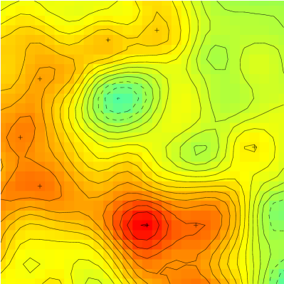
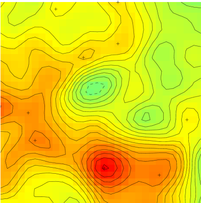
Figure 1: The same patch of the microwave sky seen without (left) and with (right) the lensing effect by the large-scale structure of a Standard Cold Dark Matter model normalized with $\sigma_{8}=1.5$. The temperature of the CMB is reflected in the temperature of the colors, and contours are drawn at intervals of 0.5 times the variance. Both the deformation of individual peaks and the distortion of the relative positions of the peaks are clearly visible.

As an example, Figure 1 shows a map with and without lensing.

3 Integral geometry for CMB maps

Minkowski functionals were formally introduced into cosmology by Mecke et al. (1994). Although the whole family of these geometric descriptors was already mentioned in (Coles, 1988), Schmalzing & Górski (1998) first applied them to CMB maps. Bernardeau (1997) suggested Minkowski functionals for detecting weak lensing signatures in the CMB. For a continuous field, we use the Minkowski functionals to describe the geometry of its excursion sets, that is the area above a given temperature threshold. In two dimensions, there are three Minkowski functionals which correspond to well-known geometrical quantities, namely the area $v_{0}$, the circumference $v_{1}$, and the Euler characteristic $v_{2}$.

The unlensed CMB maps obey Gaussian statistics. Therefore, their statistical properties can be completely characterized by the power spectrum $C_{\ell}$. Following Tomita (1990), we parametrize the Minkowski functionals of the isotemperature contour at the normalized threshold $\nu$ with $\tau$, the variance of the field’s first derivative

$$\begin{split}v_{0}^{\text{Gauss}}(\nu)&=\frac{1}{2}-\frac{1}{2}\Phi\left(\frac{\nu}{\sqrt{2}}\right),\qquad\\ v_{1}^{\text{Gauss}}(\nu)&=\frac{\sqrt{\tau}}{8}{\rm e}^{-\nu^{2}/2},\qquad\\ v_{2}^{\text{Gauss}}(\nu)&=\frac{\tau}{\sqrt{8\pi^{3}}}\nu{\rm e}^{-\nu^{2}/2}.\end{split}$$ (3)

The Appendix shows that the shapes of the Minkowski functional curves of the lensed field remain the same as in the Gaussian case. So the non-Gaussianity manifests itself only in the normalization of the curves. Let us denote the constants of proportionality from Equations (A4) and (A6) with $\alpha_{1}$ and $\alpha_{2}$, respectively. Equation (3) yields

$$\alpha_{1}^{\text{Gauss}}=\frac{\sqrt{\tau}}{8},\qquad\alpha_{2}^{\text{Gauss}}=\frac{\tau}{\sqrt{8\pi^{3}}}.$$ (4)

Therefore, for the Gaussian random field the quantity

$$\alpha=\left(\tfrac{8}{\pi}\right)^{3/2}\frac{\alpha_{1}^{2}}{\alpha_{2}}$$ (5)

equals unity. As we shall see, lensing leads to deviations from unity.

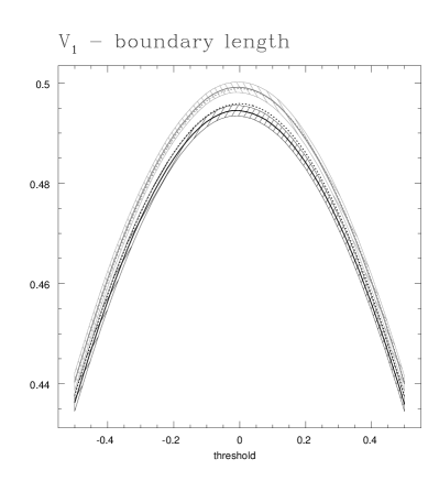
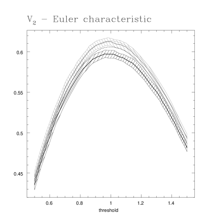
Figure 2: Minkowski functionals for the lensed and unlensed maps observed by the Planck satellite. Results for the unlensed maps are shown in grey, while black lines indicate the Minkowski functionals of the lensed maps. For both, the average and standard deviation are shown in solid lines, while the expectation values for a Gaussian random field with the same two-point characteristics are displayed in dashed lines. Note that we only show the region around the maxima of the Minkowski functional curves, where the differences are visibly significant.

Even with high resolution and large sky coverage, these changes are easily overcome by the cosmic error. Therefore, accurate evaluation of the Minkowski functionals is crucial. We use three independent methods and take care that they produce compatible results. One of them uses contour integration to evaluate the circumference and the Morse theorem (Morse & Cairns, 1969) to determine the Euler characteristic (see e.g. Novikov et al. 1999). Two more elaborate methods (Schmalzing & Buchert, 1997) evaluate the Minkowski functionals via Crofton’s formula (Crofton, 1868), and by averaging over invariants formed from derivatives, respectively. Figure 2 shows the Minkowski functionals of one of the models.

For each realization, we determine the non-Gaussianity parameter $\alpha$ by fitting the measured Minkowski functionals to their expected Gaussian shapes. Since each of our realizations covers only 15% of the sky, while for the Planck satellite a sky coverage of 60% and more is expected, we reduce our estimated variances by a factor of two. It is also worth mentioning that we assume Gaussianity of the convergence field on scales of 5’ and above. This is not exactly true (Jain et al., 2000), so we expect an even stronger signal from a refined analysis with a convergence field calculated from $N$–body simulations.

Table 1 summarizes our results. As expected, neither of the unlensed models deviates significantly from Gaussianity. For the maps that include the weak lensing effect, the average $\alpha$ is different from one. In all but one case, this difference is significant, and in two out of the four investigated models with lensing, the significance level is above 95%.

4 Discussion and Outlook

We have measured the weak lensing effect of large-scale structure on the observed temperature anisotropies of the CMB with Minkowski functionals. Numerical simulations have shown that the effect can be significant when observed with the experimental specifications of Planck. It remains to be seen whether the Minkowski functionals can directly measure any characteristics of large-scale structure. Since they are sensitive to smoothing, we expect that varying the smoothing scale can reveal information on the convergence field on different scales. Most importantly, however, we have proven that this method can measure non-Gaussian signatures induced by weak lensing at all.

Appendix A Analytical treatment

Consider a scalar random field $\psi$ in two dimensions, e.g. the observed CMB temperature anisotropy. It can be related to a scalar Gaussian random field $\varphi$, the intrinsic temperature anisotropy, through the vector-valued random field ${\boldsymbol{\xi}}$, the displacement, by Equation (1).

It is well-known that the PDF of the temperature field, and hence the zeroth Minkowski functional $v_{0}$, which is just the integrated PDF, does not change at all under lensing. We write the other two Minkowski functionals as spatial averages over invariants formed from the field’s derivatives (Schmalzing & Górski, 1998):

$$v_{1}(\nu)=\frac{\pi}{4}\left\langle{\delta(\psi-\nu)\sqrt{\psi_{,1}^{2}+\psi_{,2}^{2}}}\right\rangle,\qquad v_{2}(\nu)=\frac{1}{2\pi}\left\langle{\delta(\psi-\nu)\frac{2\psi_{,1}\psi_{,2}\psi_{,12}-\psi_{,1}^{2}\psi_{,22}-\psi_{,2}^{2}\psi_{,11}}{\psi_{,1}^{2}+\psi_{,2}^{2}}}\right\rangle.$$ (A1)

In order to evaluate these two averages, we need to express the first- and second-order derivatives of $\psi$ in terms of the fields $\varphi$ and ${\boldsymbol{\xi}}$. Straightforward differentiation yields

$$\psi_{,i}=\varphi_{,i}+\varphi_{,k}\xi_{k,i},\qquad\psi_{,ij}=\varphi_{,ij}+\varphi_{,ik}\xi_{k,j}+\varphi_{,jk}\xi_{k,i}+\varphi_{,kl}\xi_{k,i}\xi_{l,j}+\varphi_{,k}\xi_{k,ij}.$$ (A2)

For the circumference $v_{1}$, Equation (A1) involves only the first derivatives of the observed field $\psi$ and therefore, by Equation (A2), only the first derivatives of the intrinsic field $\varphi$. Since these are independent of the value $\varphi$ itself (Adler, 1981), and ${\boldsymbol{\xi}}$ is of course independent of the field $\varphi$, the average splits neatly into two factors:

$$v_{1}(\nu)=\frac{\pi}{4}\left\langle{\delta(\psi-\nu)}\right\rangle\left\langle{\sqrt{\psi_{,1}^{2}+\psi_{,2}^{2}}}\right\rangle=\frac{\pi}{4}\frac{{\rm e}^{-\nu^{2}/2}}{\sqrt{2\pi}}\left\langle{\sqrt{\psi_{,1}^{2}+\psi_{,2}^{2}}}\right\rangle.$$ (A3)

The remaining average is independent of $\nu$, so the curve has the Gaussian shape:

$$v_{1}(\nu)\propto{\rm e}^{-\nu^{2}/2}.$$ (A4)

Turning to the Euler characteristic $v_{2}$, we observe that Equation (A1) expressed in terms of the fields $\varphi$ and ${\boldsymbol{\xi}}$ depends linearly on the second derivatives $\varphi_{,ij}$ and $\xi_{k,ij}$. Therefore, $v_{2}$ depends on the threshold $\nu$ only through

$$\left\langle{\delta(\varphi-\nu)\varphi_{,ij}}\right\rangle=-\tau\nu\frac{{\rm e}^{-\nu^{2}/2}}{\sqrt{2\pi}}\delta_{ij}\qquad\text{and}\qquad\left\langle{\delta(\varphi-\nu)\xi_{k,ij}}\right\rangle=0.$$ (A5)

The remainder of the average in Equation (A1) again produces factors that do not depend on the threshold $\nu$. So the curve $v_{2}(\nu)$ also has the shape expected for the Gaussian case:

$$v_{2}(\nu)\propto\nu{\rm e}^{-\nu^{2}/2}.$$ (A6)

Table 1: The “non-Gaussianity parameter” $\alpha$ from Equation  (5). For a Gaussian random field, $\alpha$ should be unity, while deviations from one are expected for a weakly lensed CMB sky. $\alpha$ and $\Delta\alpha$ are the average and standard error over all realizations of each model.

model	experiment	$\sigma_{8}$	$\alpha$	$\Delta\alpha$
$\Lambda$CDM	Planck	no lensing	1.00019	0.00182
$\Lambda$CDM	Planck	1.0	1.00099	0.00153
$\Lambda$CDM	Planck	1.5	1.00209	0.00184
$\Lambda$CDM	Planck	2.0	1.00502	0.00186
SCDM	Planck	no lensing	0.99912	0.00171
SCDM	Planck	1.5	1.00355	0.00183

References

- Adler (1981) Adler, R. J. 1981, The geometry of random fields (Chichester: John Wiley & Sons)
- Bardeen et al. (1986) Bardeen, J. M., Bond, J. R., Kaiser, N., & Szalay, A. S. 1986, ApJ, 304, 15
- Bernardeau (1997) Bernardeau, F. 1997, A&A, 324, 15
- Bernardeau (1998) —. 1998, A&A, 338, 767
- Bond & Efstathiou (1987) Bond, J. R. & Efstathiou, G. 1987, MNRAS, 226, 655
- Burles & Tytler (1998) Burles, S. & Tytler, D. 1998, ApJ, 499, 699
- Coles (1988) Coles, P. 1988, MNRAS, 234, 509
- Crofton (1868) Crofton, M. W. 1868, Phil. Trans. Roy. Soc. London, 158, 181
- Efstathiou & Bond (1999) Efstathiou, G. & Bond, J. R. 1999, MNRAS, 304, 75
- Guth (1981) Guth, A. H. 1981, Phys. Rev. D, 23, 347
- Guth & Pi (1985) Guth, A. H. & Pi, S.-Y. 1985, Phys. Rev. Lett., 49, 1110
- Jain et al. (2000) Jain, B., Seljak, U., & White, S. 2000, ApJ, 530, 547
- Mandolesi et al. (1995) Mandolesi, N., Bersanelli, M., Cesarsky, C., Danese, L., Efstathiou, G., Griffin, M., Lamarre, J. M., Norgaard-Nielsen, H. U., Pace, O., Puget, J. L., Raisanen, A., Smoot, G. F., Tauber, J., & Volonte, S. 1995, Planetary and Space Science, 43, 1459
- Mecke et al. (1994) Mecke, K. R., Buchert, T., & Wagner, H. 1994, A&A, 288, 697
- Minkowski (1903) Minkowski, H. 1903, Mathematische Annalen, 57, 447, in German
- Morse & Cairns (1969) Morse, M. & Cairns, S. S. 1969, Critical point theory in global analysis and differential topology (New York and London: Academic Press)
- Novikov et al. (1999) Novikov, D. I., Feldman, H. A., & Shandarin, S. F. 1999, Int. J. Mod. Phys., D8, 291
- Sato (1981) Sato, K. 1981, MNRAS, 195, 467
- Schmalzing & Buchert (1997) Schmalzing, J. & Buchert, T. 1997, ApJ, 482, L1
- Schmalzing & Górski (1998) Schmalzing, J. & Górski, K. M. 1998, MNRAS, 297, 355
- Seljak (1996) Seljak, U. 1996, ApJ, 436, 1
- Seljak & Zaldarriaga (1996) Seljak, U. & Zaldarriaga, M. 1996, ApJ, 469, 437
- Sugiyama (1995) Sugiyama, N. 1995, ApJS, 100, 281
- Takada & Futamase (2000) Takada, M. & Futamase, T. 2000, accepted for publication in ApJ, astro-ph/0008377
- Takada et al. (2000) Takada, M., Komatsu, E., & Futamase, T. 2000, ApJ, 533, L83
- Tomita (1990) Tomita, H. 1990, in Formation, dynamics and statistics of patterns, ed. K. Kawasaki, M. Suzuki, & A. Onuki, Vol. 1 (World Scientific), 113–157
- van Waerbeke et al. (2000) van Waerbeke, L., Bernardeau, F., & Benabed, K. 2000, ApJ, 540, 14