$\omega$ Centauri – a former nucleus of a dissolved dwarf galaxy? New evidence from Strömgren photometry

Abstract

CCD $vby$ Strömgren photometry of a statistically complete sample of red giants and stars in the main sequence turn-off region in $\omega$ Centauri has been used to analyse the apparently complex star formation history of this cluster. From the location of stars in the $(b-y),m_{1}$ diagram metallicities have been determined. These have been used to estimate ages of different sub-populations in the color-magnitude diagram and to investigate their spatial distributions. We can confirm several earlier findings. The dominating metal-poor population around $-1.7$ dex is the oldest population found. More metal-rich stars between [Fe/H]=$-1.5$ and $-1.0$ dex tend to be 1-3 Gyr younger. These stars are more concentrated towards the cluster center than the metal-poor ones. The most-metal rich stars around $-0.7$ dex might be up to 6 Gyr younger than the oldest population. They are asymmetrically distributed around the center with an excess of stars towards the South.

We argue that the Strömgren metallicity in terms of element abundances has another meaning than in other globular clusters. From a comparison with spectroscopic element abundances, we find the best correlation with the sum C+N. The high Strömgren metallicities, if interpreted by strong CN-bands, result from progressively higher N and perhaps C abundances in comparison to iron. The large scatter of Strömgren abundances may come from a variety of evolutionary effects, including C-depletion and N-enrichment. We see an enrichment already among the metal-poor population, which is difficult to explain by self-enrichment alone.

An attractive speculation (done before) is that $\omega$ Cen was the nucleus of a dwarf galaxy. We propose a scenario in which $\omega$ Cen experienced mass inflow over a long period of time, until the gas content of its host galaxy was so low that star formation in $\omega$ Cen stopped, or alternatively the gas was stripped off during its infall in the Milky Way potential. This mass inflow could have occurred in a clumpy and discontinuous manner, explaining the second peak of metallicities, the abundance pattern, and the asymmetric spatial distribution of the most metal-rich population. Moreover, it explains the kinematic differences found between metal-poor and metal-rich stars.

1 Introduction

Since decades $\omega$ Centauri has been the target of many investigations by photometric and spectroscopic means. It is known as an extraordinary object among the star clusters of our Galaxy. $\omega$ Cen is not only the most massive and one among the most flattened Galactic globular clusters (Meylan meyl87 (1987); White & Shawl whit87b (1987)), but also shows strong variations in nearly all element abundances investigated so far (e.g. Norris & Da Costa norr95 (1995) and references therein). This is reflected by the intrinsic broad scatter of the red giant branch (already noticed in the 70s by Cannon & Stobie cann (1973)) that cannot be explained by internal reddening only (e.g. Norris & Bessell norr75 (1975)). Most recently, Pancino et al. (panc (2000)) confirmed the existence of a very metal-rich population in $\omega$ Cen whose red giant branch (RBG) is well separated from the bulk of the RGB stars.

Table 1: Observation log of $\omega$ Centauri fields

Id.	$\alpha_{2000}$	$\delta_{2000}$	Date	Exposure time [s]			seeing
				$y$	$b$	$v$
1	13:26:57.9	$-$47:33:09	1993 May 14	30,60	60,120	120,240	$1\aas@@fstack{\prime\prime}4$–$1\aas@@fstack{\prime\prime}7$
2	13:26:59.7	$-$47:38:50	1993 May 12	30,360,240	60,660,600	120,960,960	$2\aas@@fstack{\prime\prime}0$–$2\aas@@fstack{\prime\prime}5$
			1993 May 14	30	60,240	120,480	$1\aas@@fstack{\prime\prime}4$–$1\aas@@fstack{\prime\prime}6$
3	13:27:00.1	$-$47:41:52	1993 May 14	30,300,300	60,600,600	120,900,900	$1\aas@@fstack{\prime\prime}4$–$1\aas@@fstack{\prime\prime}9$
4	13:27:00.1	$-$47:46:02	1993 May 14	30,300,300	60,600,600	120,960,1020	$1\aas@@fstack{\prime\prime}4$–$1\aas@@fstack{\prime\prime}7$
5	13:27:26.3	$-$47:28:54	1993 May 13	30,300,360	60,600,720	120,960,1080	$1\aas@@fstack{\prime\prime}1$–$1\aas@@fstack{\prime\prime}4$
6	13:27:55.6	$-$47:28:01	1993 May 13	30,300,360	60,600,660	120,900,1020	$1\aas@@fstack{\prime\prime}3$–$1\aas@@fstack{\prime\prime}5$
7	13:28:21.1	$-$47:27:52	1993 May 13	30,300,360	60,600,660	120,900,1020	$1\aas@@fstack{\prime\prime}2$–$1\aas@@fstack{\prime\prime}4$
8	13:28:49.4	$-$47:27:52	1993 May 13	30,300	60,600	120,900	$1\aas@@fstack{\prime\prime}3$–$1\aas@@fstack{\prime\prime}5$
A	13:28:01.1	$-$47:28:32	1995 Apr 21	30,360	60,360	120,720	$1\aas@@fstack{\prime\prime}3$–$1\aas@@fstack{\prime\prime}6$
			1995 Apr 22	30,120	60,210	120,420	$1\aas@@fstack{\prime\prime}4$–$1\aas@@fstack{\prime\prime}7$
B	13:27:48.0	$-$47:24:06	1995 Apr 21	30,300,240	60,480,420	120,780,720	$1\aas@@fstack{\prime\prime}2$–$1\aas@@fstack{\prime\prime}6$
C	13:27:17.0	$-$47:22:26	1995 Apr 21	30,240,180	60,420,360	120,720,840	$1\aas@@fstack{\prime\prime}1$–$1\aas@@fstack{\prime\prime}3$
D	13:26:50.0	$-$47:19:06	1995 Apr 21	30,90	60,180	120,420	$1\aas@@fstack{\prime\prime}1$–$1\aas@@fstack{\prime\prime}2$
E	13:26:42.0	$-$47:24:06	1995 Apr 21	30,180	60,360	120,600	$1\aas@@fstack{\prime\prime}1$–$1\aas@@fstack{\prime\prime}2$
			1995 Apr 22	30,180,180	60,300,300	120,600,600	$1\aas@@fstack{\prime\prime}2$–$1\aas@@fstack{\prime\prime}4$
F	13:26:15.0	$-$47:26:56	1995 Apr 22	30,150,150	60,300,270	120,600,600	$1\aas@@fstack{\prime\prime}2$–$1\aas@@fstack{\prime\prime}4$
G	13:25:45.9	$-$47:26:56	1995 Apr 22	30,300,300	60,540,540	120,900,900	$1\aas@@fstack{\prime\prime}4$–$1\aas@@fstack{\prime\prime}6$
H	13:25:15.9	$-$47:26:56	1995 Apr 22	30,240,180	60,480,300	120,840,600	$1\aas@@fstack{\prime\prime}3$–$1\aas@@fstack{\prime\prime}6$
I	13:24:45.8	$-$47:26:57	1995 Apr 24	30,180	60,330	120,660	$1\aas@@fstack{\prime\prime}2$–$1\aas@@fstack{\prime\prime}3$
0	13:26:50.0	$-$47:28:33	1995 Apr 24	30	60	120	$1\aas@@fstack{\prime\prime}1$–$1\aas@@fstack{\prime\prime}2$

The abundance variations in $\omega$ Cen point to a more complicated star formation history than that for other globular clusters which contain a homogeneous stellar population. Whereas the CNO variations might be explained by evolutionary mixing effects in the stellar atmosphere as well as by mixing in the protocloud (e.g. Bessell & Norris bess76 (1976)), the iron abundance variations need another explanation (e.g. Vanture et al. vant (1994), Norris & Da Costa norr95 (1995)). The metallicity distribution of the stars in $\omega$ Cen, as derived from Calcium abundance measurements of more than 500 red giants (Norris et al. norr96 (1996)), indicates a bimodality with a distinct peak at [Ca/H] $\simeq-1.4$ dex and a shallower peak at -0.9 dex. These authors also quote statistical evidence that the more metal-rich stars are stronger concentrated towards the cluster center, as one may expect from a dissipative settling of the gas in a self-enrichment process. Similar results were obtained by Suntzeff & Kraft (sunt96 (1996)) who measured Calcium abundances of $\simeq$ 380 stars and also found a peak at [Fe/H] $=-1.7$ dex and a broad tail to higher metallicities. Their data did not support a bimodal metallicity distribution, but again a weak radial metallicity gradient. Both groups favoured an extended period of star formation connected with self-enrichment as the interpretation of their data. A dynamical analysis of 400 stars in the Norris et al. (norr96 (1996)) sample revealed a rotation of the metal poor component, whereas the metal rich one is not rotating (Norris et al. norr97 (1997)). This may be compatible with a merger of two globular clusters with different masses, as shown by the model calculations of Makino et al. (maki (1991)). However, then one would expect a metallicity distribution that is peaked at two distinct values, which is in contradiction to the continuous distribution shown by the authors.

A recent spectroscopic investigation by Smith et al. (smith00 (2000)) shows no strong signatures of enrichment by SNe Ia, but a strong increase of s-process heavy elements with iron abundances, as has been found by Norris & Da Costa (norr95 (1995)) and other studies as well. This can pose a problem, since these elements are believed to come from AGB stars (see Smith et al. smith00 (2000) for a discussion and references), and SNe Ia probably also have intermediate-age progenitors (e.g. McMillan & Ciardullo (mcmi96 (1996)).

Because of its peculiar properties, more and more authors raised the question, whether $\omega$ Cen can actually be regarded as a “true” globular cluster, or whether it is more likely the stripped nucleus of a dwarf galaxy that has been accreted by the Milky Way (Majewski et al. maje99b (1999), Lee et al. leey (1999), Hughes & Wallerstein hugh (1999)). This scenario has also been proposed for M54, one of the most massive globular clusters. It is a candidate for the nucleus of the Sagittarius dwarf galaxy (e.g. Bassino & Muzzio bass95 (1995)). Three more globular clusters might have belonged to Sagittarius (Da Costa & Armandroff daco95 (1995)), now be added to the Milky Way globular cluster system.

Similarly, the globular clusters NGC 362 and NGC 6779 might have been associated with the former host galaxy of $\omega$ Cen because of their similar, strong retrograde orbits (Dinescu et al. dine99b (1999)).

An origin of $\omega$ Cen within a dwarf galaxy outside the Milky Way could provide a natural explanation for its unique properties. Local Group dwarf spheroidals are known to have complex star formation histories (e.g. Grebel greb97 (1997)). One can imagine that this could also be true for the nuclei of dwarf galaxies which either experienced a extended period of star formation from enriched gas retained in the galaxy potential, or even were built from a merger of two clusters that spiraled into the center of the dwarf galaxy (Miller et al. mill98 (1998)). Medium-resolution spectroscopy of 25 nuclei in dwarf ellipicals of the Fornax cluster indicated that all these nuclei have a metal-rich component and some even may be sites for recent star formation (Held & Mould held (1994)).

However, whether the metallicity spread in $\omega$ Cen also is accompanied by an age spread awaits verification. In most investigations age effects cannot be disentangled from metallicity effects in the turn-off and giant branch region. Hughes & Wallerstein (hugh (1999)) observed one field in $\omega$ Cen with Strömgren $vby$ photometry which is more metallicity sensitive than broad band photometry. They report an age spread of at least 3 Gyr for stars between $-2.2<$ [Fe/H] $<-0.5$ dex (the metal-richest stars also being the youngest). However, a study of $\omega$ Cen in the Washington system combined with the DDO51 filter, which is similarly sensitive to metallicity as the Strömgren system, could not confirm this result (e.g. Majewski et al. maje99b (1999)). Further photometric and spectroscopic analysis with a high metallicity and age resolution are needed to fully understand the complex formation and enrichment history of this outstanding object.

In this paper we present CCD Strömgren $vby$ photometry of about 810 arcmin² area within $24\arcmin$ from the cluster center. Strömgren photometry has been proven to be a very useful metallicity indicator for globular cluster giants and subgiants (e.g. Richter et al. richp (1999), Hilker hilk00a (2000), Grebel & Richtler greb92 (1992), Richtler rich89 (1989)). The location of late type stars in the Strömgren $(b-y),m_{1}$ diagram is correlated with their metallicities, especially with their iron and CN abundances. A new Strömgren metallicity calibration for red giants is presented by Hilker (hilk00a (2000)). With our observations we are able to determine Strömgren metallicities of a statistically complete number of red giants in $\omega$ Cen and study their spatial distribution.

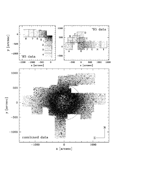
Figure 1: The lower panel shows the position plot of all observed fields in $\omega$ Centauri. All stars with a $V$ magnitude brighter than 19.0 mag and a photometric error less than 0.1 mag have been plotted. Bold dots indicate the position of all stars with determined metallicities (see Fig. 4). The indicated circle (at 10 arcmin radius) is a selection criterium for the analysis of the angular distribution of the RGB stars. The upper panel shows the positions and nomenclature (see Table 1) of the long exposures in the ’93 run (left) and the ’95 run (right). Only stars with $V<16.0$ have been plotted

In Sect. 2 we present the observations and data reduction. Sect. 3 presents color magnitude diagrams and selection criteria that have been used to determine the metallicity distribution from the $(b-y),m_{1}$ diagram (Sect. 4). In Sect. 5 the red giants in $\omega$ Cen have been divided into sub-populations, whose ages and spatial distribution have been analysed. Finally, Sect. 6 suggests a formation history for $\omega$ Cen and Sect. 7 summarises the results.

2 Observations and data reduction

The observations of $\omega$ Centauri have been performed in two observing runs in 1993 and 1995 with the Danish 1.54m telescope (direct imaging) at ESO/La Silla. In both runs, the CCD in use was a Tektronix chip with 1024$\times$1024 pixels. The $f$/8.5 beam of the telescope provides a scale of $15\aas@@fstack{\prime\prime}7$/mm, and with a pixel size of 24 $\mu$m the total field is $6\aas@@fstack{\prime}3\times 6\aas@@fstack{\prime}3$. In the first run, 11.-15. May 1993, 8 fields have been observed through the Strömgren $vby$ filters. The nights were not always photometric, and the seeing, measured by the FWHM of stellar images, was in the range $1\aas@@fstack{\prime\prime}1$–$2\aas@@fstack{\prime\prime}5$ (see Table 1). In the second run, 21.-24. April 1995, 10 fields have been taken. All nights had photometric conditions, and the seeing varied between $1\aas@@fstack{\prime\prime}1$–$1\aas@@fstack{\prime\prime}7$. The observation log of both runs is given in Table 1 and the position of the fields are illustrated in Fig. 1. Additionally, 20 fields with short exposures have been observed in order to cover the spectroscopic sample of 40 red giants (Norris & Da Costa norr95 (1995)), which have been included in a new Strömgren metallicity calibration (Hilker hilk00a (2000)). The observation and data reduction of these fields is described in Hilker (hilk00a (2000)).

The CCD frames were processed with standard IRAF routines, instrumental magnitudes were derived using DAOPHOT II (Stetson stet87 (1987), stet92 (1992)). For the comparison with the standard stars, aperture–PSF shifts have been determined in all fields. The remaining uncertainty of this shift is in the order of 0.01 mag in all filters. For the ’95 run the corrected magnitudes of the stars belonging to overlapping areas of two adjacent fields agree very well and have been avaraged for the final photometry file. For the photometric reference the ’95 run have been chosen, since the ’93 run was not continuously photometric. The instrumental magnitudes determined in this run have been transformed to those of ’95 using stars belonging to overlapping areas. The calibration of the combined sample was done via standard stars by Jønch-Sørensen (jonc93 (1993), jonc94 (1994)) obtained in the ’95 run. The calibration equations and coefficients are given in Richter et al. (richp (1999)), in which the Strömgren photometry of M55 and M22 is presented. All Strömgren colors refer to the photometric system defined by Olsen (olse93 (1993)).

After the photometric reduction, combining of the data sets, and calibration of the magnitudes, the average photometric errors for the red giants used for the metallicity determination are 0.012 mag for $V$, 0.016 mag for $(b-y)$ and 0.025 mag for $m_{1}$.

3 The Color Magnitude Diagram (CMD)

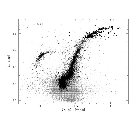
Figure 2: Color magnitude diagram of all observed stars in $\omega$ Cen with a photometric error of less than 0.1 mag (grey) and of less than 0.03 mag (black) in $y$ and $b$. The broad red giant branch cannot be explained by photometric errors, but is due to a spread in metallicity and probably age. Bold dots are definite cluster members by their radial velocities.

Figure 2 shows the $(b-y)$ versus $V$ color magnitude diagram of all observed stars in $\omega$ Cen with a photometric error less than 0.1 mag ($\simeq$ 91450 stars, grey dots) and less than 0.03 mag ($\simeq$ 20620 stars, black dots) in $y$ and $b$. Furthermore about 300 definite cluster members, on the basis of their radial velocities (Norris et al. norr97 (1997), Suntzeff & Kraft sunt96 (1996)) are marked with bold dots. The colors have been corrected for a reddening value of $E_{B-V}=0.11$ mag (Zinn zinn85 (1985), Webbink webb (1985), Reed et al. reed (1988), Gonzalez & Wallerstein gonz (1994)). This corresponds to $E_{b-y}=0.08$ and $E_{m_{1}}=-0.02$, using the relations of Crawford & Barnes (craw (1970)), $E_{b-y}=0.7E_{B-V}$ and $E_{m_{1}}=-0.3E_{b-y}$. The broad red giant branch (RGB) cannot be explained by photometric errors or internal reddening. The dispersion in the blue horizontal branch (BHB) along the reddening vector in the range $-0.01<(b-y)_{0}<0.05$ and $14.5<y_{0}<14.8$ is 0.037 mag. The expected photometric error in the same direction is 0.017 mag. Thus, internal reddening should be in the order $E_{b-y}\leq 0.02$ mag, or $E_{B-V}\leq 0.03$, consistent with what already was found by Norris & Bessell (norr75 (1975)). The dispersion of the RGB in the same magnitude bin and $0.47<(b-y)_{0}<0.57$ is 0.051 mag, significantly higher than that at the BHB. At other magnitudes the dispersion orthogonal to the RGB is as follows: $12.0<y_{0}<12.4$: 0.078 (0.013), $13.2<y_{0}<13.6$: 0.055 (0.016), and $16.3<y_{0}<16.7$: 0.035 (0.025). In brackets the expected photometric errors are given. Note that the dispersion increases from the lower towards the upper RGB.

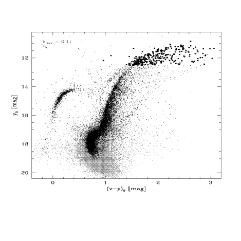
Figure 3: Color magnitude diagram with $(v-y)_{0}$ as color for the same stars as in Fig. 2. Note the larger scale in color as compared to Fig. 2. The large spread in this CMD is dominated by the CN variations in the cluster stars. The CN-normal stars of the metal-poor population clearly define a narrow sequence at the blue side of the RGB

Since the $(b-y)$ color as a metallicity indicator is not affected by CN variations, the spread in the RGB must be due to a spread in the overall metallicity (iron abundance) and/or age. It is interesting to note that a remarkable number of stars is located redwards of the apparent “main” RGB, which cannot be explained by foreground stars only (a lot of them are definite members, see Fig. 2). Their existence in this CMD points to a small population of stars that are significantly more metal-rich than the majority of the stars in $\omega$ Cen (see also Pancino et al. panc (2000)).

The situation changes when plotting the $(v-y)_{0}$ color versus $y_{0}$ (see Fig. 3). The red giants cover a much wider color range. In this CMD the scatter towards redder colors is not only due to different metallicities and ages, but is mainly dominated by the CN variations, since the $v$ filter is sensitive to the CN band strength. Whereas CN-rich stars scatter to redder colors, the CN-normal stars with a low metallicity clearly define a sharp sequence at the blue side of the RGB. Thus, the combination of both diagrams can be used to separate the metal-poor CN-normal stars from CN-rich ones (see next section) and study their properties. Note also that in the $(v-y)$,$y$ CMD the asymptotic giant branch (AGB) is more clearly separated from the RGB than in the $(b-y)$,$y$ CMD.

3.1 The redness parameter

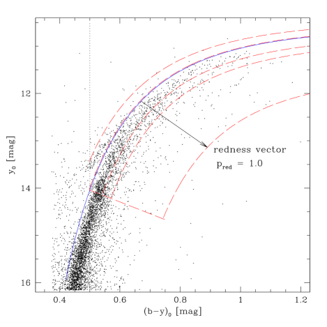
Figure 4: In this color magnitude diagram all stars with $V_{0}<16.0$ mag, $(b-y)_{0}>0.35$, a photometric error less than 0.05 mag are plotted. All stars which are enclosed by the dashed lines were used for the metallicity determination ($\simeq$ 1500 stars). The solid line indicates a fit to the blue envelope of the RGB that has been used to define the zero line for a redness parameter (see text)

As mentioned in the previous section the displacement of giants from the “main” RGB towards redder colors in the $(b-y),y$ CMD reflects their higher metallicity, but does not depend on the CN anomalies. In order to quantify this deviation we defined a parameter that measures the distance of a red giant in the CMD from the blue envelope of the RGB along the reddening vector. The blue envelope was parameterized by the following function,

$y_{0}=a_{0}+a_{1}/(b-y)_{0}+a_{2}/(b-y)_{0}^{2}$

with the parameters $a_{0}=10.917$, $a_{1}=-1.308$, and $a_{2}=1.436$. This in the following called “redness” parameter $p_{\rm red}$ is illustrated in Fig. 4. For illustrative purposes, we distinguish between 4 “populations”. Stars that are located bluewards of the RGB ($=$ negative $p_{red}$) mainly are AGB stars (P1). The RGB is divided into three subsamples: a blue (P2; $-0.01<p_{\rm red}<0.17$) and a red (P3; $0.17<p_{\rm red}<0.29$) side of the RGB, and all stars that are redder than the “main” RGB (P4; $0.29<p_{\rm red}<1.0$).

4 The two-color diagram and metallicity distribution

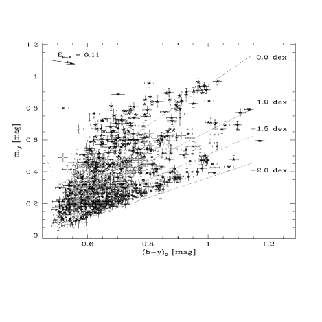
Figure 5: In this plot the $(b-y),m_{1}$ diagram for about 1500 selected giants (see Fig. 4) is shown together with the lines of constant metallicity from the recent calibration by Hilker (hilk00a (2000)). The error bars include photometric and calibration errors. The black dots indicate stars from the blue side of the RGB (P2), grey triangles the ones from the red RGB side (P3), and asterisks all stars lying apart from the “main RGB” (P4). Light grey squares indicate AGB stars (P1). The dotted line marks the selection criterium for the metallicity distribution shown in Fig. 6 (lower panel)

Figure 6: In the upper panel the metallicity distribution of about 1500 red giants is shown together with the division into subsamples (according to Fig. 4). Stars from the blue side of the RGB peak around $-$1.7 dex. AGB stars (more densly hashed) even are more metal-poor. Red RGB stars mainly range between $-1.3$ and $-0.5$ dex, whereas most of the “reddest” stars scatter to higher metallicities. Note that most of the stars with metallicities higher than $-$0.8 stars are CN-rich stars. In the lower panel about 1120 stars with a higher accuracy in their metallicity determination (stars redder than the dotted line in Fig. 5) have been selected. The solid and dashed lines represent the analysis of the metallicity distribution using a density estimation technique (kernel estimator with an Epanechnikov kernel). A second peak at about $-$0.9 dex becomes prominent

The $(b-y),m_{1}$ diagram (Fig. 5) is indicative for the metallicity distribution and CN variations of the red giants in $\omega$ Cen. The selected 1500 red giants (see Fig. 4) show a large scatter between $-2.0$ and 1.0 dex in their Strömgren metallicity. The Strömgren metallicity is defined as

$${\rm[Fe/H]}_{\rm ph}=\frac{m_{1,0}-1.277\cdot(b-y)_{0}+0.331}{0.324\cdot(b-y)_{0}-0.032}$$ (1)

following the calibration by Hilker (hilk00a (2000)). The trend exists that stars on the blue side of the RGB are mostly metal-poor, whereas the stars redwards of the “main” RGB populate the metal-rich regime, as one would expect if no CN-anomaly was present. This trend becomes even more pronounced, if the stars are plotted in a metallicity histogram. The upper panel in Fig. 6, where [Fe/H]_ph denotes the Strömgren metallicity, shows the distribution of all selected stars. A peak around $\simeq-1.7$ dex with a sharp cutoff towards low metallicities at $-1.9$ dex represents the blue RGB stars (P2). Also most of the AGB stars (P1) bluewards the main RGB belong to this metal-poor population. Stars from the red side of the RGB (P3) have metallicities mainly in the range $-1.3$ to $-0.5$ dex. If stars with a low accuracy (stars bluer than the dotted line in Fig. 5) are skipped, the P3-stars appear well separated from the metal-poor population and define a second peak at about $-0.9$ dex (see lower panel, Fig. 6), resembling the results of Norris et al. (norr96 (1996)). Stars with Strömgren metallicities higher than about $-0.8$ dex are supposed to be CN-rich stars of one of the two populations, since no stars with an iron abundance higher than that has been found in the cluster. However, many of them are redder than the “main” RGB. Since their $(b-y)$ color is not influenced by CN variations, their existence in the CMD can only be explained by higher iron abundances. In the upper panel of Fig. 6 the numbers in the metallicity histogram represent about the correct proportion of metal-poor to metal-rich stars, since the stars have been selected due to a luminosity cut in the CMD (see Fig. 4). The metal-poor population in $\omega$ Cen dominates the metal-rich one by a ratio of about 3:1.

4.1 Strömgren metallicity versus Fe, C and N abundance

The metallicity distribution found in our investigation is qualitatively very similar to that found by Norris et al. (norr96 (1996)) and Suntzeff & Kraft (sunt96 (1996)) from their Calcium abundance measurements. In Fig. 7 we show the metallicity distribution of those stars that are in common in both samples. The Calcium abundances from Suntzeff & Kraft (upper panel) have been transformed to iron abundances according to the relation given in their paper.

The behaviour of $\omega$ Cen regarding its relation between Fe abundance and Strömgren metallicity is remarkably different from that of other globular clusters (open circles in the lower panel of Fig. 7, including NGC 6334, NGC 3680, NGC 2395, NGC 6397, M22 and M55, taken from Hilker hilk00a (2000)).

The straight relation up to -1 dex (with large scatter towards higher metallicities) is in striking contrast, for example, to the situation in M22 (Richter et al. richp (1999)), where there is a considerable scatter at a fixed iron abundance. What determines the Strömgren colors in $\omega$ Cen? An answer may come from a comparison of the available elements abundances for 40 giants from Norris & Da Costa (norr95 (1995)), which in part also entered the calibration of Hilker (hilk00a (2000)) with our Strömgren colors. Fig. 8 shows in four panels the Strömgren metallicity vs. [Fe/H], [C/H], [N/H], and [C+N/H]. It is apparent that the correlation with [Fe/H] and [C/H] is very poor. It is better for [N/H] (note the large error of 0.4 dex given for the N-abundance by Norris & Da Costa (norr95 (1995)), and best for [C+N/H].

Figure 7: The two plots show the metallicity distribution of those red giants that are in common with the samples of Norris et al. (norr96 (1996), upper panel) and Suntzeff & Kraft (sunt96 (1996), lower panel). In the upper panel the calcium abundance is plotted versus [Fe/H]_ph, in the lower one the iron abundance as derived from the calcium abundance using the results of Norris & Da Costa (norr95 (1995)). In both panels the dotted lines indicate the detected peaks in the metallicity distributions. The solid line in the lower panel is the iso-metallicity line. Whereas most stars of the metal-poor peak and the mean metallicities of globular clusters from the literature are located close to this line, basically all more metal-rich stars clearly deviate from this relation in a systematic manner (dashed relations). The CN over-abundance is dominated by the C abundances and seems to be correlated to the enrichment process of iron.

Figure 8: The spectroscopically determined iron, nitrogen, carbon and nitrogen+carbon abundances of red giants in $\omega$ Cen (Norris & Da Costa (norr95 (1995)) are plotted versus their Strömgren metallicity. Whereas the correlation with [Fe/H] and [C/H] apparently is very poor, it is better for [N/H] (Norris & Da Costa give an error of 0.4 dex fot their N-abundances) and best for [C+N/H]

On the other hand, there is a close correlation of [Fe/H] vs. [C+N/H] (Fig. 9) (which, by the way, is suprising, given the above large error of the N abundance). The two most deviating stars are ROA 139 and ROA 144. They have the highest N-abundances in this sample, simultaneously low oxygen abundances and hence are probably strongly affected by mixing effects.

If we skip them, a linear regression returns $0.64\pm 0.07$ for the slope, indicating that the increase in C+N is faster than in [Fe/H]. Can this be understood as a stellar evolutionary effect? As Norris & Da Costa point out, C-depletion as a signature of the CNO-cycle is present and one may see the increase in the C-abundance with [Fe/H] in their Fig.8a to have its cause in the decreasing efficiency of the mixing-up of processed material with increasing metallicity, as it is theoretically expected (e.g. see Kraft kraf94 (1994)). But then, the increase in C+N is not easy to understand, since it is dominated by an increase of N, where we would expect a decrease, and, after all, the sum of C and N should be less sensitive to mixing effects.

A further striking fact is that we see in Fig. 7 the relation between [Fe/H] and Strömgren metallicity already present among the old population, where it is hard to understand that such small differences in [Fe/H] would cause a regular pattern in the mixing effects. We thus propose that the gradual enrichment of C+N, indicated by the Strömgren colors, is to a large degree primordial (we use the term “primordial” as the alternative to mixing effects).

The suggestion that a part of the proto-cluster material of $\omega$ Cen has undergone considerable C-enrichment has also been made by e.g. Cohen & Bell (cohe86 (1986)) and Norris & Da Costa (norr95 (1995)) based on the unique presence of CO-strong stars. Moreover, the [C/Fe] abundance in the metal-poor population is about $-$0.7 dex according to Norris & Da Costa, which is close to $-$0.5 dex, theoretically expected from the yield ratios in SNe II (Tsujimoto et al. tsuj95 (1995)). If, say, $-$0.2 dex would be the “true” value of [C/H], one would require a considerable C-contribution from intermediate-age stars, which by itself is not easy to understand for the first stars formed in $\omega$ Cen. Also a mean [O/C]-value of approximately $-$1 dex, as one would read off from Norris & Da Costa is close to the theoretically expected yield ratios from SNe II.

Figure 9: The spectroscopically determined iron abundance is plotted versus the sum of nitrogen+carbon abundances of red giants in $\omega$ Cen (Norris & Da Costa (norr95 (1995)). The slope of $0.64\pm 0.07$ indicates a faster increase in [C+N/H] than in [Fe/H]. See text for further comments

On the other hand, if the increasing [C+N/Fe] among the metal-poor old population was, at least to large part, primordial, one is driven to the conclusion that the star formation process, which formed these stars, did not took place in a single burst within a well-mixed environment, but must have been extended in time, allowing intermediate-age populations to contribute.

We shall attempt to combine these abundance pattern with other properties within a consistent scenario later on.

4.2 Metallicities in the MSTO region

The Strömgren $m_{1}$ index also is sensible to metallicity for stars around the main sequence turn-off (MSTO) region. A recent calibration has been published by Malyuto (maly (1994)) which is valid in the color ranges $0.22<(b-y)_{0}<0.38$ and $0.03<m_{1,0}<0.22$ (the above considerations regarding the C-sensitivity do not necessarily apply here since the CN-band influence is less in these hotter stars). Hughes & Wallerstein (hugh (1999)) applied this calibration to their Strömgren data of $\omega$ Cen and showed that the stars of different metallicity bins hardly differ in the location at the MSTO region (see their Fig. 9 and 10). There exists the trend that the more metal-rich stars seem to be bluer in average than the metal-poor ones, in contrast to what one would expect if all stars had the same age. Applying Malyuto’s calibration to our data we confirm this finding, as shown in Sect. 5.1. In Fig. 11 (right panels) the location of MSTO stars for three different metallicity bins is shown. Since our sample is not complete in this magnitude range and photometric errors are large, we hesitate to attempt a quantitative analysis of the metallicity distribution in the MSTO region. But it is apparent that the more metal-rich stars cannot be fit by old isochrones.

5 Analysis of sub-populations in $\omega$ Cen

The combination of the redness parameter $p_{\rm red}$ and the Strömgren metallicity [Fe/H]_ph can be used to divide the RGB in different sub-populations and examine their ages and their spatial distribution in the cluster. In Fig. 10 a plot of $p_{\rm red}$ versus [Fe/H]_ph is shown. As mentioned in the previous section there exists the general trend that the reddest stars also are tho most metal/CN-rich ones as it is expected. The solid diagonal line in this diagram shows the expected relation between $p_{\rm red}$ and [Fe/H]_ph if the stars would behave according to the calibration of Hilker (hilk00a (2000)) (“CN-normal stars”). Besides the asymptotic giant branch, three sub-populations have been selected (boxes with solid lines) that define different parts of the giant branch in the CMD. Confirmed member stars of $\omega$ Cen according to their radial velocities are spread all over the parameter space (dark dots). Hence a separation of non-member stars in this diagram is hardly possible. Later on, we will use further sub-selections within the sub-populations (dashed and dotted areas) to examine the different spatial distributions within $\omega$ Cen.

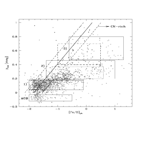
Figure 10: The redness parameter $p_{\rm red}$ is plotted versus the Strömgren metallicity. Dark dots mark member stars according to their radial velocities. The boxes with solid lines define different sub-populations of the red giants in $\omega$ Cen which have been used for age determination (see Fig. 11). The solid diagonal line shows the expected relation between $p_{\rm red}$ and [Fe/H]_ph for CN-normal stars. The dashed lines are the error boundaries for $\pm 0.3$ dex. Stars within the dotted boxes in the populations 1) and 2) have been used for the examination of their cumulative radial distribution (see Fig. 14). In the dashed boxes stars are selected for the angular distribution shown in Fig. 15

5.1 Age estimation of sub-populations

For the identification of possibly different ages among the sub-populations of $\omega$ Cen the isochrones from Bergbusch & VandenBerg (berg (1992), in the following BV92) have been used, converted to Strömgren colors by Grebel & Roberts (greb95 (1995)).

The location of the metal-poor giants in the CMD has been used to define a reference isochrone. Adopting their known metallicity ([Fe/H]$=-1.7$ dex), a distance modulus, color offset, and age has been determined. For fitting the RGB, only stars with a photometric error less than 0.025 mag in $y$, $b$ and $v$ are selected. The error in metallicity of these stars is less than 0.3 dex. In the MSTO region stars with a color error less than 0.03 mag in $(b-y)$ and 0.04 mag in $m_{1}$ have been selected to determine the location of the isochrone.

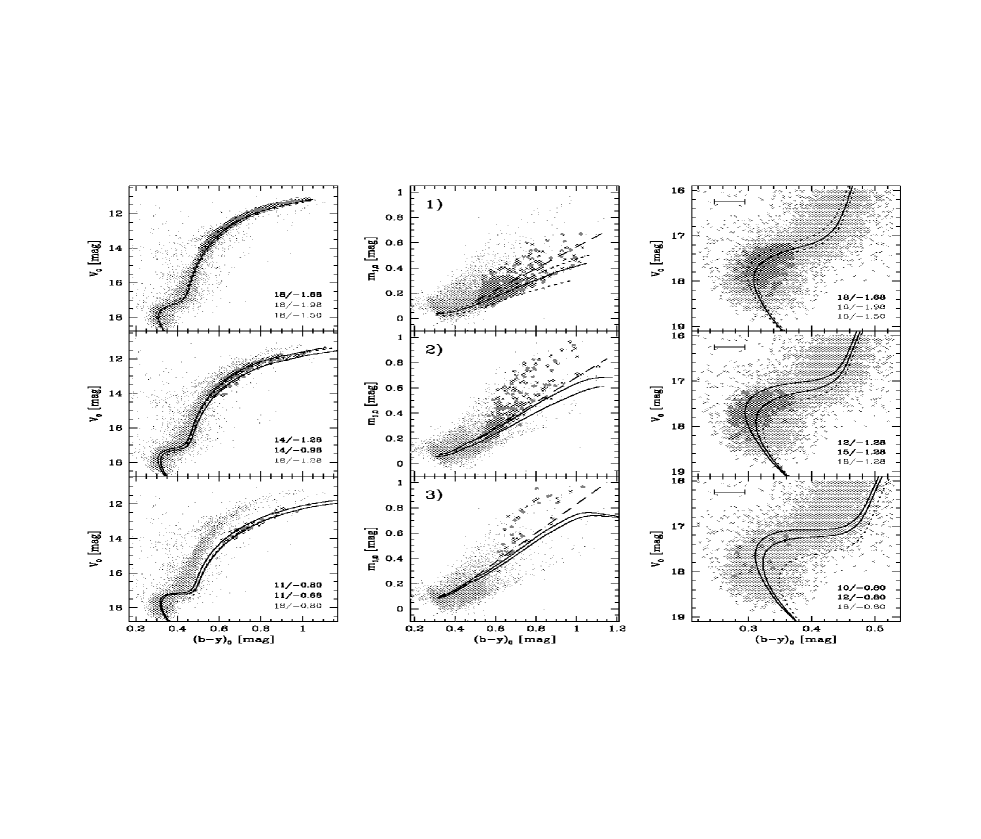
Figure 11: This figure shows the age and metallicity estimation of three selected sub-populations (vertical arrangement) in the RGB (dark dots, left panels) and MSTO region (dark triangles, right panels) of $\omega$ Cen (see boxes in Fig. 10). Only RGB stars with a photometric error less than 0.025 mag in $y$, $b$ and $v$ and MSTO stars with errors less than 0.03 mag in $(b-y)$ were selected (the mean error bar is indicated in the upper left corner of the right panels). The error in metallicity of the selected RGB stars is less than 0.3 dex. The left and right panels show the CMDs of the RGB and MSTO region with the best fitting isochrones for the corresponding sub-population overlayed. The isochrones are those from Bergbusch & VandenBerg (berg (1992)), converted to Strömgren colors by Grebel & Roberts (greb95 (1995)). In the uppermost panels the adopted reference isochrone and two boundary isochrones (dotted) are shown that fit the MSTO region of the metal-poor stars and follow the shape of their RGB. In the other panels, the dotted isochrone has the same age as the reference isochrone, but with a metallicity that fits the location of the RGB stars in the corresponding selection. Ages and metallicities of the isochrones are given in the lower right corners of the plots (thin letters are for the dotted isochrones). There exists not only an increase in metallicity when going to redder giant branches, but also a sequence towards younger ages. Isochrones with high metallicities, but older ages do not fit the MSTO region. The same isochrones also have been used in the middle panels, where the $(b-y),m_{1}$ diagram is shown. The old isochrones cannot be distinguished in their location from their younger counterparts of the same metallicity. The redder the giant branch the higher is the ratio of stars that do not follow the isochrones as determined in the CMD, but show enhanced CN abundances ($=$ all stars above the dashed lines which indicates about the separation between CN-normal and CN-strong stars). The results of the isochrone fitting are summarized in Fig. 12

The best fitting isochrone for [Fe/H]$=-1.7$ dex is shown in the upper panels of Fig. 11 (solid line). A distance modulus of $(m-M)_{0}=13.57$ mag and additional necessary offsets in $(b-y)$ of $[(b-y)_{0}-(b-y)_{\rm iso}]=-0.037$ mag and in $m_{1,0}$ of $[m_{1,0}-m_{1,\rm iso}]=0.005$ were used. The age that fits best the MSTO region and follows the shape of the RGB is 18 Gyr. We note that this isochrone does not perfectly fit the color of the RGB but is slightly redder which might be due to uncertainties in the color transformations of this set of isochrones to observational data. Moreover, we are aware of the fact that the absolute age has to be corrected towards younger ages when applying more recent sets of isochrones (i.e. VandenBerg et al. vand00 (2000)), but, unfortunately, newly calculated isochrones in the Strömgren system still are missing.

In comparison to the selected reference isochrone, relative ages and metallicities ($=$ iron abundances) of the other sub-populations in $\omega$ Cen have been determined (see Fig. 11). Whereas the color of the RGB stars is quite sensitive to metallicity, but not to age, the metallicity selected stars in the MSTO region can constrain the age (see also results of Hughes & Wallerstein hugh (1999)).

The main (blue) part of the RGB, called population 1) and defined by $0.04<p_{\rm red}<0.18$ and $-2.0<$[Fe/H]${}_{\rm ph}<-0.1$, corresponds to the reference isochrones. This population can be fit by isochrones in the metallicity range $-2.0<$[Fe/H]${}_{\rm ph}<-1.4$ dex and ages between 16 and 18 Gyr. Although all stars in this metallicity range might be fit by the same age (see dotted lines in the upper panels of Fig. 11), there exists the tendency that the more metal-rich stars seem to be better fit by the younger isochrones (see Fig. 12). Stars with higher Strömgren metallicities than -1.3 dex (see $(b-y),m_{1}$ diagram in Fig. 11) cannot be fit by isochrones with the corresponding metallicities. For the same ages these isochrones would be too red in the RGB region, for younger ages they are too blue in the MSTO region. Thus, these stars are most probably CN-rich stars of the old, metal-poor population.

Population 2), defined by $0.20<p_{\rm red}<0.46$ and $-1.4<$[Fe/H]${}_{\rm ph}<1.0$, lies beyond the main RGB region redwards of pop 1). Best fitting isochrones range between $-1.4$ and $-1.0$ dex. Only few stars show these metallicities in the $(b-y),m_{1}$ diagram, reflecting the fact that most of them are CN-strong. The age of this population ranges between 12 and 16 Gyr. Older isochrones with metallicities around $-1.3$ dex do not fit the MSTO region (see dotted isochrone in the right middle panel of Fig. 11). Isochrones with higher metallicities than $-1.0$ dex do not fit pop 2) at any age.

The last defined population 3), with $0.47<p_{\rm red}<0.80$ and $-0.6<$[Fe/H]${}_{\rm ph}<1.3$, stands apart from the broad main sequence, but nevertheless contains confirmed cluster members (see Fig. 10) and was clearly detected in the large sample of Pancino et al. (panc (2000)). Isochrones that fit this population are in the range $-0.8$ to $-0.6$ dex and around 10–12 Gyr. Older isochrones with [Fe/H]$=-0.8$ dex do not fit the MSTO region.

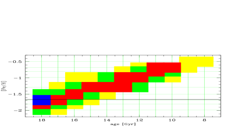
Figure 12: In this plot the age-metallicity relation for stellar populations in $\omega$ Cen is shown. The grid represent the set of isochrones used (Bergbusch & VandenBerg berg (1992)). The black square defines the adopted reference isochrone. Dark grey areas are the age and metallicity combinations that fit the CMD of $\omega$ Cen best. Middle grey areas are less probable due to their displacement either in the RGB or the MSTO region, and light grey are isochrones at the margin of the MSTO region, either to the blue or to the red side. The horizontal line at $-1.68$ dex marks the peak of the metallicity distribution (see Fig. 6)

The results of the age determination is summarized in Fig. 12. In the grid of the isochrone set dark grey areas mark the best fitting isochrones in comparison to the reference isochrone (black square). Isochrones represented in light grey marginally fit the borders of the MSTO and/or RGB region for the selected stars of a particular metallicity. There obviously exists an age metallicity relation in the sense that the more metal-rich stars tend to be younger. Whereas all stars of the main RGB with metallicities between $-2.0$ and $-1.4$ dex might be compatible with one age, the populations with metallicities around $-1.2$ and $-0.7$ dex are at least 2–5 and 5–8 Gyr younger. If the age metallicity relation in $\omega$ Cen can be understood as a continuous enrichment process after an initial starburst with [Fe/H]$\simeq-1.7$ dex, the age spread of the enrichment lies between 5 and maximally 8 Gyr. We note that the latest isochrones sets (e.g. VandenBerg et al. vand00 (2000)) give absolute ages that are about 2-5 Gyr younger than that of Bergbusch & VandenBerg (berg (1992)) at a given magnitude and color. Also the relative age differences would result smaller so that, in fact, the age spread of the populations in $\omega$ Cen might not be that large as indicated above.

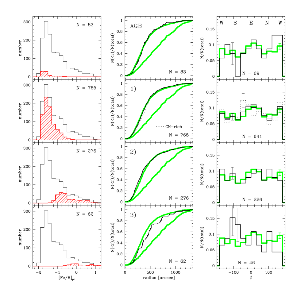
Figure 13: The left panels show the Strömgren metallicity distribution of different sub-populations of red giants in $\omega$ Cen, selected according to the solid boxes shown in Fig. 10. As reference the distribution of all giants is shown. In the middle panels the cumulative radial distributions of the populations is shown. The grey lines represent reference distributions of the whole giant sample and probable non-member stars. Distributions marked with black solid and dashed lines are metallicity sub-selections as labeled in the plots. The division into CN-normal (thin solid line) and CN-rich stars (dotted line) in panel 1) is according to the selection in Fig. 10. The differences of the radial profiles between the metal-poor stars from pop1 and the CN-rich stars from pop2 and pop3 is highlighted in Fig. 14. The angular distribution of the corresponding sample selections is shown in the right panels. The number counts in the angular bins are normalised to the total number in each sample. Only stars within a radius of $10\arcmin$ have been selected. The distribution of all selected stars is plotted as grey histogram for reference. Error bars indicate the average statistical errors of the corresponding selection in one bin. In all plots the number of selected stars is given.

5.2 Spatial distribution of red giants

The same sub-populations, as defined for the age determination, have been used to investigate the spatial distribution of their stars. Additionally, the AGB stars have been included. In Fig. 13 the metallicity distribution (left panels), the cumulative radial distribution (middle panels), and the angular distribution (right panels) of all selections are shown. Only stars within the area indicated in Fig. 4, with photometric errors less than 0.05 mag and errors in the metallicity determination less than 0.4 dex have been selected. A central circular area with a radius of $30\arcsec$ have been excluded because of incompleteness in this area. The metallicity distribution of all selected stars ($=1448$) is shown as reference in the left panels. The cumulative profiles of these stars and 160 probable non-members are shown as grey lines in the middle panels. The non-members have been selected according to: $14.5<y_{0}<16.5$ and $0.1<(b-y)_{0}<0.4$. For plotting the angular distribution, we included only stars within a radius of $10\arcmin$ from the cluster center. The number counts have been normalised to the total number for each selection. The angle $\phi$ is defined as $0\degr$ in East direction, $+90\degr$ North, and $-90\degr$ South. The histogram of all stars ($=1186$ giants, grey histogram in the right panels, Fig. 13) shows the reference distribution function in the selected area.

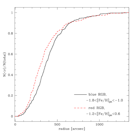
Figure 14: This plot shows the cumulative distribution of different subsamples of red giants in a 20$\arcmin$ broad East-West strip which is perpendicular to the rotation axis. The selection of the subsamples is illustrated in Fig. 10 (dotted regions). The metal-richer and younger stars (dashed line) are more concentrated than the old metal-poor population (solid line). The probability that both populations follow the same radial distribution is less than 0.1% (according to a KS test)

The population of the selected 83 AGB stars is very metal-poor with a small fraction of CN-strong stars (see Fig. 13, upper left panel). Therefore, they most probably belong to the old metal-poor population in $\omega$ Cen. Also their cumulative radial distributions resemble closely that of pop 1). A Kolmogorov-Smirnov (KS) test gives a 98% probability that both radial distributions are equal. Deviations in the angular distribution are statistically not significant as shown by the error bar.

When comparing population 1) with population 2) there seems to be a slight difference in their radial distributions in the sense that the ratio of the metal-rich to metal-poor (pop2:pop1) is higher in the cluster center than in its outskirts. This result is statistically significant as discussed below and shown in Fig. 14. The angular distribution of both sub-populations do not differ significantly from each other. Within the metal-poor population 1) there exists only a marginal difference between the 542 selected CN-normal and 209 CN-rich stars in their spatial distributions.

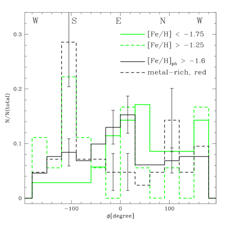
Figure 15: The angular distributions of the most metal-poor (solid histograms) and most metal-rich (dashed histograms) giants in $\omega$ Cen are shown. The number counts are normalized to the total number in each sample. The grey distributions represent the samples by Jurcsik (jurc (1998)). Black histograms contain stars selected on the basis of our photometric metallicity determinations (selection areas, see dashed boxes in Fig. 10). Errorbars indicate the statistical error in the corresponding bins. The excess of very metal-rich stars in the South direction could be confirmed. However, metal-poor stars seem not to be segregated towards the North, but show the same number counts in South and North direction

In Fig.14 the higher concentration of the more metal-rich stars is highlighted. In this plot only stars in an E-W-strip with a N-S-extension of 20$\arcmin$ have been selected, since these fields belong to the most homogeneous set of long exposures. 500 metal-poor giants are compared with 190 giants of the more metal-rich population (selections see dotted boxes in Fig. 10). A KS test reveals a probablity of less than 0.1% that the cumulative number counts of both populations follow the same radial distribution.

The radial distribution of the stars in pop 3) appears less concentrated than the average cluster population. Some of them might be solar metallicity foreground stars. However, others are confirmed cluster member stars. The angular distribution of pop 3) shows a concentration of stars towards the South and a slight depression in the West and North direction which can explain the different radial distribution. In this context we note that Jurcsik (jurc (1998)) reported on a spatial metallicity asymmetry in $\omega$ Cen. Taking all stars with known iron abundances, either directly measured or derived from [Ca/H] values, she found that the most metal-rich stars with [Fe/H]$>-1.25$ dex are concentrated towards the South, whereas the most metal-poor stars with [Fe/H]$<-1.75$ are more concentrated in the North. In order to check this result, two sub-samples have been defined that match the two selections by Jurcsik in our [Fe/H]${}_{\rm ph},p_{\rm red}$ plane (dashed boxes in Fig. 10). In Fig. 15 the angular distributions are shown. The sample of Jurcsik (light grey histograms) contains 35 metal-poor and 18 metal-rich stars that are in common with our photometric sample. The high concentration of the most metal-rich stars in the South is confirmed by our selection of 42 metal-rich stars. It even is more pronounced. Nearly 30% of the sample are located in the Southern angular bin. A KS test reveals a probability of 94% that the metal-rich stars from the Jurcsik and our sample have the same angular distribution. However, we cannot confirm an asymmetrical distribution in the North-South direction of the 131 selected most metal-poor stars. There exists an excess of stars towards the East which might be explained by the high ellipticity of this population, but number counts in the North and in the South are the same. The probability that the angular distribution of the metal-poor stars of Jurcsik’s and our sample agree is less than 7% (KS test). Also less than 7% is the probability that metal-rich and metal-poor stars are distributed equally.

6 Problems and a scenario

Can the younger populations in $\omega$ Cen be enriched by the older one? In trying to answer this we use oxygen as a tracer for the synthesized material. First we estimate the number of SNe type II having occured in the old population. If we adopt the mass of $\omega$ Cen to be $4\times 10^{6}$ solar masses (Pryor & Meylan pryor93 (1993)), the metal-poor population comprises about $2.8\times 10^{6}$ solar masses. Now we assume a Salpeter mass function (exponent $-$2.3) between 0.1 and 100 solar masses. Then we can calculate the number of expected SNe II, if we furthermore assume that each star more massive than 10 solar masses explodes as SN II. We get 45000 SNe. This number would be (perhaps considerably) higher, if the actual mass function was shallower than a Salpeter mass function at lower masses, for which there is evidence (Paresce & De Marchi pare00 (2000)). The total oxygen mass released by these SNe is about 50000 solar masses, (based on Table 7.2 of Pagel pagel97 (1997)). On the other hand, following Norris & Da Costa norr95 (1995), a mean [O/H] value for the metal-rich population is -0.7 dex (adopting [O/Fe] = 0.5 dex and [Fe/H] = $-$1.2 dex), so we calculate the actual oxygen mass to be 2300 solar masses, if the total mass of the young population is $1.2\times 10^{6}$ solar masses. Since Smith et al. (smith00 (2000)) see no signature of enrichment by SNe Ia, it is reasonable to assume that the oxygen mass, which was present already in the gas before the enrichment, scales with the iron abundance. The difference is approximately a factor of 3, so we have 1500 solar masses of newly synthesized oxygen in the metal-rich population. This means that only 3% (and probably much less) of the released oxygen has been retained. If we do that exercise with the iron abundance, we have 1000 solar masses of iron released (Pagel pagel97 (1997), S. 158), and we have about 20 solar masses of newly synthesised iron present. Of course, the exact numbers are insignificant, but they demonstrate that practically all material must have been blown out.

This is also plausible from the energy point of view. We have a release of kinetic energy by about $5\times 10^{54}$ erg from the SNe (neglecting previous stellar winds and ionizing radiation), while the binding energy of the “proto-young population” is about $2\times 10^{52}$ erg, if we for simplicity imagine that the gas was confined within an half-light radius of 7 pc (Djorgovski djor93 (1993)).

Similar factors must apply for the overall fraction of retained gas, implying an unreasonable large protocluster mass (neglecting the problem how a bound system could survive with such low star formation efficiency), if one wants to live with a permanently retained large gas fraction.

But we have even more problems. Smith et al. (smith00 (2000)) do detect only weak signatures of SNe Ia, expressed by the low [Cu/Fe] value of -0.6 dex. On the other hand, both the age spread, the increase of s-process elements, and the interpretation of the Strömgren results as primordial enrichment of C and N speak for the contribution of an intermediate-age population. Within 3-4 Gyr, at least some Ia events should have been ocurred, making the problem with the low iron content even worse, if they would have provided iron to the young population. Why do we not see their debris?

Moreover, it is remarkable that we find the signature of intermediate-age populations already among the old population, indicated by the evidence that the same relation between [Fe/H] and Strömgren metallicity (Fig. 7), which connects the oldest and the younger population, appears already to be present at the lowest metallicities. The general behaviour of the Strömgren metallicities resembles in this respect the well established enrichment of s-process elements relative to iron. Unfortunately, the sample of spectroscopically studied stars is still too small to allow a definite statement also for the metal-poor population, but Fig.12 of Norris & Da Costa (norr95 (1995)) indicates that there might be an increase of barium relative to iron already at low metallicities. How can these stars, in a regular pattern, be self-enriched simultaneously by SNe II and by intermediate-age stars?

It may be that one can construct a scenario in which these oddities can be explained by pure self-enrichment (see for instance Smith et al. smith00 (2000)). However, we wish to point out an alternative, which has not yet been mentioned and which seems to offer an easier way towards an understanding of $\omega$ Cen.

The above problems arise under one certain assumption, namely that $\omega$ Cen formed out of a gaseous protocluster of the appropriate mass, which had for a long time a high gas-to-star ratio. If we (speculatively) drop this assumption, then the problems are less severe.

The previously expressed hypothesis that $\omega$ Cen was the nucleus of a dwarf galaxy, gains much attractivity in this context. We additionally speculate that its star formation rate was triggered galaxy. We additionally speculate that its star formation rate was triggered over a very extended period (perhaps more than 5 Gyr) by mass supply from the overall gas reservoir of its host galaxy. This scenario can explain all characteristic properties of $\omega$ Cen found so far.

This gas inflow, already enriched in the host galaxy, could have occured in a non-spherical, clumpy and discontinuous manner, providing angular momentum and thus giving rise to the flattening of $\omega$ Cen. We have no problems with the competition of gas removal and simultaneous enrichment. The intermediate-age population stars in $\omega$ Cen released their gas, for instance by planetary nebulae, in a much less violent fashion and the infalling gas can mix with this C and N rich material, which also was rich in s-process elements, giving rise to a new star formation period. The large scatter in the Strömgren metallicities may thus be in part primordial, reflecting the incomplete mixing of the infalling gas with the C-N-rich material. Both SNe II,Ib and Ia would sweep up the gas almost completely, terminating star formation for a short while, until further mass infall becomes possible.

It also seems natural that younger and more metal-rich populations show other kinematic and spatial properties, including asymmetries in their spatial distribution, depending on the details of the infall process. We would then expect many periods of strong star formations alternating with periods of mass infall. The mass infall would finally cease after the gas content of the host galaxy has become sufficiently low or was perhaps removed by ram presure stripping in the Galactic halo during its infall in the Milky Way (e.g. Blitz & Robishaw blit (2000)). One is tempted to ask, whether $\omega$ Centauri could have evolved to a object resembling the bulge of a spiral galaxy, if its host galaxy would have been more massive.

The subsequent evolution can be sketched as follows: on its retrograde orbit the dwarf galaxy spiraled towards the Galactic center (Dinescu et al. dine99b (1999)). On its way it lose the outermost stellar populations by tidal stripping, including the two likely member globular clusters NGC 362 and NGC 6779 (Dinescu et al. dine99b (1999)). Finally, after its stellar population dissolved totally, the nucleus $\omega$ Cen remained and appears now as the most massive cluster of our Milky Way.

A strong motivation for the above scenario comes from the C+N enrichment relative to iron of the metal-poor population. It would therefore be of extreme interest to have a larger sample of metal-poor stars (possibly main sequence stars) spectroscopically analysed to see whether this feature can also be seen in the s-process elements.

7 Summary and Conclusions

For about 1500 red giants in $\omega$ Centauri Strömgren metallicities have been determined. Almost 2/3 of them turn out to be metal-poor, with a peak in the metallicity distribution at [Fe/H]${}_{\rm ph}=-$1.7 dex. This finding is consistent with previous result by other authors (e.g. Norris et al. norr96 (1996), Suntzeff & Kraft sunt96 (1996)). In the CMD, this population is best fit by old isochrones (17-18 Gyr: Bergbusch & VandenBerg berg (1992)). The identifiable AGB stars seem to belong to this population according to their low metallicities and small fraction of CN-strong stars. The metallicity range in the main RGB is about $-1.9<$[Fe/H]$<-1.5$ dex. However all stars of this population are consistent with a single old age, there might exist an age spread of maximally 2 Gyr in the sense that the more metal-rich stars are younger.

Beyond the strongly peaked metal-poor population, the metallicity distribution shows a sharp cutoff towards lower metallicities, but a broad, long tail towards higher Strömgren metallicities. Most of these stars are CN-rich. Among them, a second major population ($\simeq 1/4$ of the whole population), peaks around [Fe/H]${}_{\rm ph}=-$0.9 dex, defines a giant branch redwards the main RGB that is best fit by an iron abundance around $-1.2$ dex and ages 2-5 Gyr younger than that of the oldest population. Isochrones with older ages do not fit the location of the main sequence turn-off region.

In the CMD of $\omega$ Cen there exists a red giant branch far redwards from the main RGB that contains proven cluster member stars according to their radial velocities. This population exhibits less than 5% of the whole cluster population. The best fitting isochrones have an iron abundance around $-0.7$ dex and ages 5-8 Gyr younger than the oldest population. Strömgren metallicities of most of them ($\ga$80%) are significantly higher than $-0.7$ dex, identifying them as CN-strong stars.

The comparison between [Fe/H] abundances derived from high-dispersion spectroscopy of Norris & Da Costa (norr95 (1995)) and Strömgren metallicities shows a behaviour distinctly different from that observed in other globular clusters. There is hardly a correlation with [Fe/H], but a close correlation with [C+N/H].

However, the comparison of Strömgren metallicities to the larger sample of Suntzeff & Kraft (sunt96 (1996)) shows that there is a coupling to the iron abundance indicating that this has a primordial cause. It is already visible among the metal-poor population and we interpret it as another manifestation of the well established increasing contribution of intermediate-age populations with increasing iron abundance.

The comparison of the cumulative radial distribution of the two main populations in $\omega$ Cen exhibits a higher concentration of the metal-rich stars within a radius of $10\arcmin$ from the cluster center. The youngest, most metal-rich population has an asymmetrical distribution around the cluster center with a concentration towards the South. Jurcsik (jurc (1998)) argues that the strong asymmetry of the most metal-rich stars in $\omega$ Cen points towards a relatively recent effect, since an initial ($>15$ Gyr) spatial metallicity anisotropy could not have been preserved that clearly. However, Meylan (meyl87 (1987)) calculated that the relaxation time of $\omega$ Cen beyond the half-mass radius ($r_{h}=2\aas@@fstack{\prime}6$) is 20-30 Gyr, compared to 1 Gyr within the core radius ($r_{c}=4\aas@@fstack{\prime}8$). Since most of the metal-rich stars are located around or beyond the half-mass radius and furthermore seem to be 5-8 Gyr younger than the old population in $\omega$ Cen, an initially asymmetric distribution of them is probably still not relaxed.

Our findings are consistent with a scenario in which enrichment of the cluster has been taken place over a period of at least 3 Gyr and maximally 6 Gyr. The conditions for such an enrichment can perhaps be found in nuclei of dwarf galaxies, where a secondary star formation is common (Grebel greb97 (1997)). All characteristic properties of $\omega$ Cen (flattening, abundance pattern, age spread, kinematic and spatial differences between metal-poor and metal-rich stars) could be understood in the framework of a scenario, where infall of previously enriched gas occured in $\omega$ Cen over a long period of time. Only the enrichment of nitrogen, carbon, and s-process elements took place within $\omega$ Cen, where the infalling gas mixed with the expelled matter from AGB stars.

The capture and dissolution of a nucleated dwarf galaxy by our Milky Way and the survival of $\omega$ Cen as its nuclues would thus be an attractive explanation for this extraordinary object. Several recent publications also support this idea and rule out other possibilities like a chemically diverse parent cloud or a merger of two clusters (e.g. Majewski et al. maje99b (1999), Lee et al. leey (1999), Hughes & Wallerstein hugh (1999)).

- (1) Bassino L.P., Muzzio J.C., 1995, Observatory 115, 256
- (2) Bergbusch P.A., VandenBerg D.A., 1992, ApJS 81, 163 (BV92)
- (3) Bessell M.S., Norris J., 1976, ApJ 208, 369
- (4) Blitz L., Robishaw T., 2000, ApJ submitted
- (5) Cannon R.D., Stobie R.S., 1973, MNRAS 162, 207
- (6) Cohen J.G., Bell R.A., 1986, ApJ 305, 698
- (7) Crawford D.L., Barnes, J.V. 1970, AJ 75, 978
- (8) Da Costa G.S., Armandroff T.E., 1995, AJ 109, 2533
- (9) Dinescu D.I., Girard T.M., van Altena W.F., 1999, AJ 117, 1792
- (10) Djorgovski S., 1993, in ”Structure and Dynamics of Globular Clusters”, ASP Conf. Ser. 50, eds. S.G. Djorgovski and G. Meylan, BookCrafters Inc., San Francisco, p.373
- (11) Gonzalez G., Wallerstein G., 1994, AJ 108, 1325
- (12) Grebel E.K., 1997, RvMA 10, 29
- (13) Grebel E.K., Richtler T. 1992, A&A 253, 359
- (14) Grebel E.K., Roberts W.J., 1995, AAS 186, 0308
- (15) Held E.V., Mould J.R., 1994, AJ 107, 1307
- (16) Hilker M., 2000, A&A 355, 994
- (17) Hughes J.D., Wallerstein G., 1999, AJ 119,1225
- (18) Jønch-Sørensen H., 1993, A&AS 102, 637
- (19) Jønch-Sørensen H., 1994, A&AS 108, 403
- (20) Jurcsik J., 1998, ApJ 506, L113
- (21) Kraft R.P., 1994, PASP 106, 553
- (22) Lee Y.-W., Joo J.-M., Sohn Y.-J., Rey S.-C., Lee H.-C., Walker A.R., 1999, Nature 402, 55
- (23) Makino, J., Akiyama, K., Sugimoto, D., 1991, Ap&SS 185, 63
- (24) Malyuto V., 1994, A&AS 108, 441
- (25) Majewski S.R., Ostheimer J.C., Kunkel W.E., Patterson R.J., 1999, AJ submitted
- (26) McMillan R.J., Ciardullo R., 1996, ApJ 473, 707
- (27) Meylan G., 1987, A&A 184, 144
- (28) Miller B.W., Ferguson H.C., Lotz J., Stiavelli M., Whitmore B.C., 1998, ApJ 508, L133
- (29) Norris J., Bessell M.S., 1975, ApJ 201, L75 (erratum in 210, 618)
- (30) Norris J.E., Da Costa G.S., 1995, ApJ 447, 680
- (31) Norris J.E., Freeman K.C., Mayor M., Seitzer P., 1997, ApJ 487, L187
- (32) Norris J.E., Freeman K.C., Mighell K.J., 1996, ApJ 462, 241
- (33) Olsen E.H., 1993, A&AS 102, 89
- (34) Pagel B.E.J. 1997, Nucleosynthesis and Chemical Evolution of Galaxies, Cambridge University Press
- (35) Pancino E., Ferraro F.R., Bellazzini M., Piotto G., Zoccali M., 2000, ApJ in press
- (36) Paresce F., De Marchi G., 2000, ApJ 534, 670
- (37) Pryor C., Meylan G. 1993, in ”Structure and Dynamics of Globular Clusters”, ASP Conf.Ser. 50, eds. S.G. Djorgovski and G. Meylan, BookCrafters Inc., San Francisco, p.357
- (38) Reed B.C., Hesser J.E., Shawl S.J., 1988, PASP 100, 545
- (39) Richter P., Hilker M., Richtler T., 1999, A&A 350, 476
- (40) Richtler T., 1989, A&A 211, 199
- (41) Smith V.V., Suntzeff N.B., Cunia K., Gallino R., Busso M., Lambert D., 2000, AJ 119, 1239
- (42) Stetson P.B., 1987, PASP 99, 191
- (43) Stetson P.B., 1992, in: ”Astronomical Data Analysis Software and Systems I, A.S.P. Conference Series, Vol. 25, eds. D.M. Worrall, C. Biemesderfer, and J. Barnes, p. 297
- (44) Suntzeff N.B., Kraft R.P., 1996, AJ 111, 1913
- (45) Tsujimoto T., Nomoto K., Yoshii Y., Hashimoto M., Yanagida S., Thielemann F.-K., 1995, MNRAS 277, 945
- (46) VandenBerg D.A., Swenson F.J., Rogers F.J., Iglesias C.A., Alexander D.R., 2000, ApJ 532, 430
- (47) Vanture A.D., Wallerstein G., Brown J.A., 1994, PASP 106, 835
- (48) Webbink R.F., 1985, in Dynamics of Star Clusters, IAU Symposium 113, eds. J. Goodman & P. Hut, Dordrecht: Reidel, p. 541
- (49) White R.E., Shawl S.J., 1987, ApJ 317, 246
- (50) Zinn R., 1985, ApJ 293, 424