Abundance analysis of two extremely metal-poor stars from the Hamburg/ESO Survey

Abstract

We report on the first high spectral resolution analysis of extremely metal-poor halo stars from the Hamburg/ESO objective-prism survey (HES). The spectra were obtained with UVES at VLT-UT2. The two stars under investigation (HE 1303–2708 and HE 1353–2735) are main-sequence turnoff-stars having metal abundances of $\mbox{[Fe/H]}=-2.85$ and $-3.20$, respectively. The stellar parameters derived from the UVES spectra are in very good agreement with those derived from moderate-resolution follow-up spectra. HE 1353–2735 is a double-lined spectroscopic binary.

The two stars nicely reproduce the strong scatter in [Sr/Fe] observed for extremely metal-poor stars. While we see a strong Sr II $\lambda 4215$  Å line in the spectrum of HE 1303–2708 ($\mbox{[Sr/Fe]}=-0.08$), we can only give an upper limit for HE 1353–2735 ($\mbox{[Sr/Fe]}<-1.2$), since the line is not detected. We report abundances of Mg, Ca, Sc, Ti, Cr for both stars, and Co, Y for HE 1303–2708 only. These abundances do not show any abnormalities with respect to known trends for metal-poor stars.Lithium is also detected in these stars, to a level which places them among Lithium-plateau metal-poor dwarfs.

1 Introduction

The most metal-poor stars carry the fossil record of the chemical compostion of the Galaxy, and hence allow one to study the ealiest epochs of Galactic chemical evolution. Moreover, there are also cosmological applications for metal-poor stars, e.g. the determination of the primordial Lithium abundance (Spite and Spite 1982; Ryan et al. 2000), constraining the baryon density parameter, or individual age determinations (e.g., Cowan et al. 1999), thus setting a lower limit to the age of the Universe. Therefore, in the past decade there has been a fast-growing interest in these stars within the astronomical community. With VLT-UT2 and UVES now being in operation, it has become feasible to study large samples of metal-poor stars at high resolution and high $S/N$ in a very reasonable time.

For the past decade, the major source of metal-poor stars has been the so-called HK survey of Beers and collaborators (Beers et al. 1985, 1992; Beers 1999) . Now, an even larger survey volume within which to search for metal-deficient stars has been opened up by use of the digital objective-prism spectra of the Hamburg/ESO Survey (HES; Wisotzki et al. 1996; Reimers and Wisotzki 1997; Wisotzki et al. 2000), since the HES is more than one magnitude deeper than the HK survey. Christlieb (2000) has shown that the selection of metal-poor candidates in the HES by automatic spectral classification is much more efficient than the manual selection applied to the HK survey, so that the amount of telescope time needed for follow-up spectroscopy is reduced, and a full exploitation of the $\sim 8\times$ larger HES volume (compared to the HK survey alone) becomes feasible. An alternative selection method in the HES is the so-called Ca K index method (Christlieb et al. 1999), which looks for stars characterized by a Ca II K line weaker than expected for their $B-V$ color. This method is almost as efficient in selecting metal-poor stars as automatic classification (Christlieb et al. 2000).

In this paper we report on the first high-resolution observations of metal-poor stars from the HES. Two stars, HE 1303–2708 and HE 1353–2735, were observed with VLT-UT2 in the course of UVES Science Verification in February 2000.

2 HES candidate selection and spectroscopic follow-up

The two stars described in this paper were selected by the Ca K-index method (Christlieb et al. 1999). As is obvious from Fig. 1, HE 1303–2708 and HE 1353–2735 were both selected because they show no Ca II K ($\lambda\,3933$  Å) line in the HES spectra.

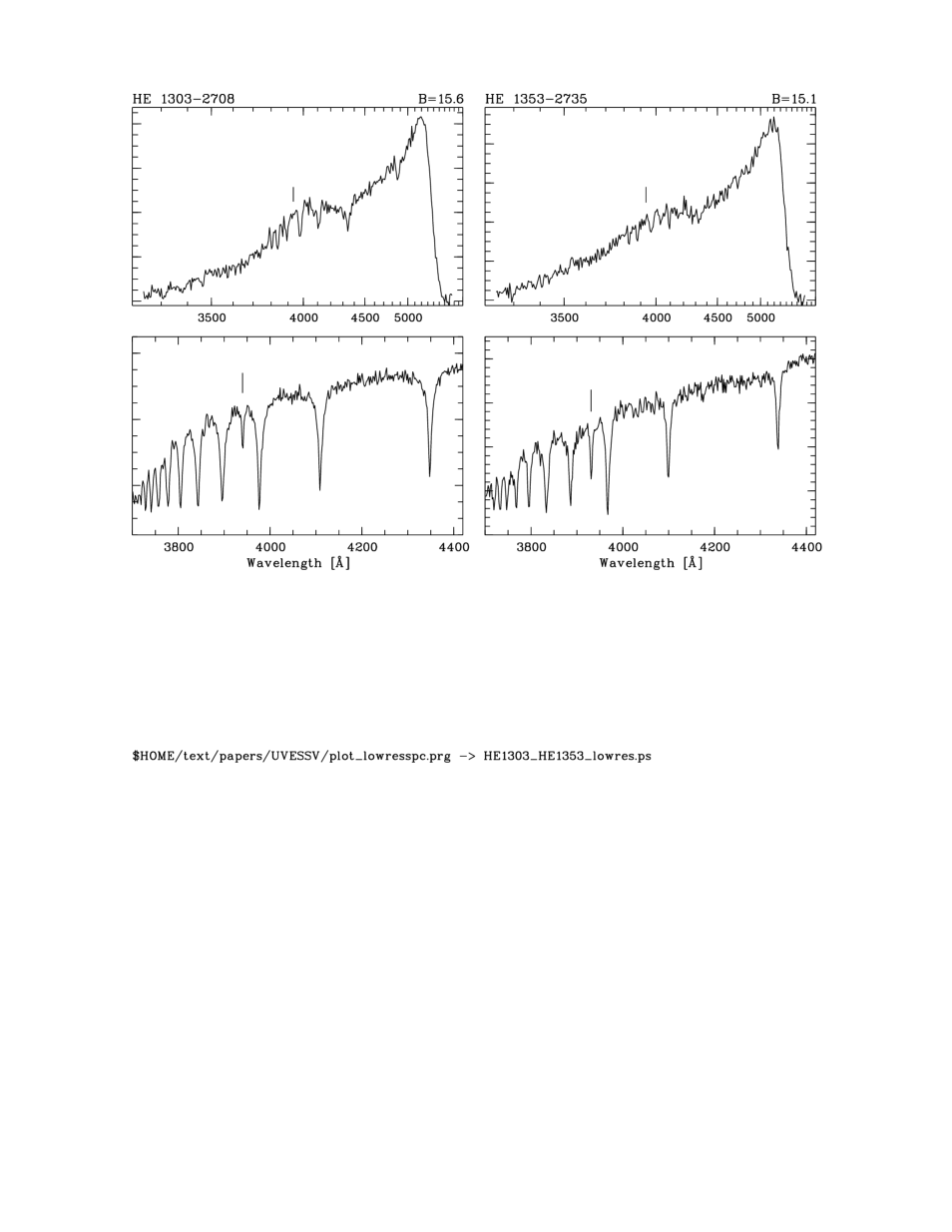
Figure 1: Upper panels: HES objective-prism spectra of HE 1303–2708 and HE 1353–2735; lower panels: Moderate-resolution spectra obtained with the ESO-NTT and EMMI. The position of Ca K is marked. The ordinates are photographic density in arbitrary units (upper panels), and relative flux (lower panels).

Tab. 1 lists coordinates (derived from the DSS-I, see e.g. http://archive.eso.org/dss/dss), and photometry for the two stars.

Table 1: Coordinates, photometry and stellar parameters for the two metal-poor stars. Photometry was derived directly from the HES plates (for the calibrations see Christlieb 2000), with the exception of $B-V$ for HE 1353–2735, which was measured in April 2000 with NTT/EMMI. Stellar parameters were derived from moderate-resolution follow-up spectra. In the second row for each star we list the $1\sigma$ errors.

Name	$\alpha(2000)$	$\delta(2000)$	$B_{J}$	$V$	$B-V$	$U-B$	$c_{1}$	$T_{\mbox{\scriptsize eff}}$	$\log g$	$\mbox{[Fe/H]}_{\mbox{\scriptsize HES}}$	$\mbox{[Fe/H]}_{\mbox{\scriptsize HK}}$
HE 1303–2708	13 06 37.8	$-$27 24 22	15.5	15.3	0.45	$-0.18$	0.49	6500 K	4.2	$-2.8$	$-3.3$
			0.2	0.2	0.03	0.09	0.15	200 K	0.5	0.2	0.2
HE 1353–2735	13 56 42.5	$-$27 49 54	15.0	14.7	0.38	$-0.27$	0.23	6000 K	4.8	$-2.9$	$-3.4$
			0.2	0.2	0.07	0.09	0.15	200 K	0.5	0.2	0.2

Spectroscopic follow-up observations were obtained in April 1999 using EMMI attached to the ESO-NTT. From these moderate-resolution ($\sim 5\,$ Å FWHM), but good quality spectra (see Fig. 1), having $S/N\sim 50$ at Ca II K and $S/N>60$ at the Mg I b triplet ($\lambda\lambda\,5167,5173,5184$  Å), the stellar parameters listed in Tab. 1 were derived via the spectrum synthesis technique. Ca K, Mg I b and Balmer line wings were used as indicators for metallicity, gravity and effective temperature, respectively. Plane-parallel LTE model atmospheres of Reetz et al. (1999, priv. comm.) were used. The analysis was performed strictly differentially to the Sun, and the well-known Calcium-overabundance of $\sim 0.4$ dex for metal-poor stars (see e.g. Wheeler et al. 1989) was taken into account.

By re-observing and re-analysing a couple of metal-poor stars from the HK survey (Beers 1999, priv. comm.), it turned out that there is an average difference of $0.5$ dex between the HES and HK survey [Fe/H] scales (Christlieb and Beers 2000), in the sense that stars appear to be more metal-poor in the HK survey than in the HES. Unfortunately it is not possible to identify the physical reason for this difference, because Beers et al. (1999) use average [Fe/H] values from the literature (which were hence determined by using many different model atmospheres) to calibrate their method. In order to make the HES metallicities comparable with those of Beers et al. (1999), we also list scaled [Fe/H] values in Tab. 1.

3 UVES observations

The observations were performed from February 10 to 18, 2000, as part of the VLT-UT2 Science Verification of UVES, the UV and Visual Echelle Spectrograph recently commissioned (D’Odorico et al. 2000). The data from this program were made public to the ESO community in April 2000 (see www.eso.org/science/ut2sv/UVES_SV.html). The spectrograph setting (Dichroic mode, central wavelength 4700  Å in the blue arm, and 7850  Å in the red arm) provided a wavelength coverage of 4100–5300  Å and 6000–9700  Å, and the entrance slit of 1$\arcsec$ yielded a resolving power of R$\sim$45 000. Table 2 gives a short log of the observations, together with the achieved $S/N$.

Table 2: Log-book of the UVES observations. $S/N$ refers to the signal-to-noise ratio per 0.025  Å pixel, at 5200  Å and 6700  Å for the blue and red spectra, respectively.

Star	Setting	$V$ [mag]	$t$ [min]	$S/N$
HE 1303–2708	B470		225	70
HE 1303–2708	R785	15.3	290	150
HE 1353–2735	B470		180	55
HE 1353–2735	R785	14.7	180	120

The spectra were reduced using the UVES context within MIDAS, which performs bias subtraction (object and flat-field), inter-order background subtraction (object and flat-field), optimal extraction of the object (above the sky, rejecting cosmic ray hits), division by a flat-field frame extracted with the same weighted-profile as the object, wavelength calibration and rebinning to a constant step and merging of all overlapping orders. The spectra were then corrected for barycentric radial velocity and co-added, and finally normalised. Fig. 2 is an example of the reduced spectrum around the magnesium triplet for both stars.

As can be noted in that figure, it turned out that HE 1353–2735 is a double-lined binary with a faint system of lines shifted to the red by $\sim 25$ ${\rm km\>s^{-1}}$. To serve as first epoch for future follow-up of the system, we note that the radial velocities observed for the two components are $v_{\mbox{\scriptsize rad,A}}=-213.8$ ${\rm km\>s^{-1}}$and $v_{\mbox{\scriptsize rad,B}}=-187.7$ ${\rm km\>s^{-1}}$, at $\mbox{MJD}=51584.31030$.

Figure 2: Mg I triplet region for both HES stars. Note that HE 1353–2735 is a double-lined binary, as can be seen from the faint lines displaced towards the red of the main lines of the spectrum. The spectrum of HE 1303–2708 was shifted vertically by 0.2 units in relative flux.

4 Stellar parameters and abundances

Table 3: Line by line abundances for all elements observed in HE 1303–2708 and HE 1353–2735, except iron. We do not list equivalent widths for HE 1353–2735, since the abundances for this star were derived from spectrum synthesis.

Element	$\lambda$	$\chi_{ex}$	$\log$ gf	W1303	$\varepsilon_{1303}$	$\varepsilon_{1353}$
	[Å]	[eV]		[mÅ]
Li I	6707.766	0.00	0.00		2.12	2.06
	6707.916	0.00	$-$0.30		2.12	2.06
Mg I	4702.998	4.34	$-$0.37	13.6	4.86
	5167.360	2.71	$-$0.86	74.4	5.19	4.8
	5172.688	2.71	$-$0.38	85.8	4.92	4.8
	5183.603	2.72	$-$0.16	95.8	4.90	4.8
Ca I	4226.740	0.00	$-$3.36			3.5
	4289.372	1.88	$-$0.30	5.9	3.71
	4302.526	1.90	0.28	20.3	3.75
	4318.649	1.90	$-$0.21	7.4	3.74
	4434.951	1.89	$-$0.01	12.8	3.78
	4454.769	1.90	0.26	20.4	3.77	3.1
Sc II	4246.823	0.31	0.32	27.3	0.40
	4314.080	0.62	$-$0.10	12.1	0.64	$-$0.2
	4320.720	0.61	$-$0.26	6.4	0.49
Ti II	4290.213	1.16	$-$1.10	15.3	2.63
	4300.042	1.18	$-$0.75	29.9	2.70	2.2
	4301.908	1.16	$-$1.43	9.2	2.72
	4395.033	1.08	$-$0.65	37.9	2.68	2.2
	4399.754	1.24	$-$1.27	9.3	2.62
	4417.716	1.16	$-$1.42	12.5	2.84
	4443.800	1.08	$-$0.81	25.8	2.55	2.1
	4468.492	1.13	$-$0.77	29.1	2.64	1.8
	4501.274	1.12	$-$0.86	28.4	2.70	2.0
	4533.957	1.24	$-$0.76	26.6	2.66	2.2
	4549.614	1.58	$-$0.47			2.3
	4563.753	1.22	$-$0.95	23.0	2.74	2.2
	4571.969	1.57	$-$0.52	27.4	2.74	2.1
Cr I	4254.333	0.00	$-$0.11	24.3	2.58	2.2
	4274.793	0.00	$-$0.23	19.1	2.55	2.2
	4289.712	0.00	$-$0.36	13.1	2.48	2.2
	5206.061	0.94	0.02	15.7	2.97
	5208.400	0.94	0.16	16.1	2.84	2.2
Co I	4121.308	0.92	$-$0.32	8.9	2.72
Sr II	4215.520	0.00	$-$0.17	40.5	$-$0.03	$<-1.5$
Y II	5087.367	1.08	$-$0.17	2.6	0.21
Ba II	4554.045	0.00	0.17	15.2	$-$0.75	$<-1.5$
	4934.080	0.00	$-$0.16	9.4	$-$0.70

Table 4: Iron abundances in HE 1303–2708 and HE 1353–2735.

Element	$\lambda$	$\chi_{ex}$	$\log$ gf	W2708	$\varepsilon_{2708}$	$\varepsilon_{2735}$
	[Å]	[eV]		[mÅ]
Fe I	4118.545	3.57	0.21	15.9	4.90
	4132.052	1.61	$-$0.67	33.5	4.55	4.5
	4143.403	3.05	$-$0.20	8.0	4.52
	4143.866	1.56	$-$0.51	42.9	4.57	4.5
	4181.736	2.83	$-$0.37	11.0	4.65	4.3
	4187.040	2.45	$-$0.55	13.6	4.61	4.5
	4187.792	2.43	$-$0.55	16.1	4.68	4.3
	4191.425	2.47	$-$0.67	8.2	4.50	4.3
	4199.090	3.05	0.16	17.4	4.55	4.3
	4202.024	1.48	$-$0.71	37.9	4.58	4.5
	4210.321	2.48	$-$0.93	4.0	4.43
	4227.430	3.33	0.27	12.4	4.50
	4233.582	2.48	$-$0.60	15.2	4.74	4.2
	4235.935	2.43	$-$0.34	17.6	4.52	4.3
	4250.112	2.47	$-$0.41	18.1	4.63	4.3
	4250.782	1.56	$-$0.71	33.9	4.55	4.5
	4260.476	2.40	0.08	35.8	4.54	4.4
	4271.149	2.45	$-$0.35	18.6	4.57	4.3
	4271.757	1.49	$-$0.16	65.8	4.72	4.5
	4282.405	2.18	$-$0.78	11.4	4.51	4.4
	4294.110	1.49	$-$1.11	35.9	4.92	4.3
	4299.230	2.43	$-$0.41	16.4	4.54	4.4
	4307.896	1.56	$-$0.07	74.3	4.91	4.3
	4315.104	2.20	$-$0.97			4.3
	4325.760	1.61	0.01	68.0	4.70	4.5
	4375.921	0.00	$-$3.03	8.9	4.70	4.3
	4383.545	1.48	0.20	7.5	4.65	4.5
	4404.746	1.56	$-$0.14	0.2	4.59	4.3
	4415.118	1.61	$-$0.61	7.6	4.57	4.5
	4427.305	0.05	$-$2.92	6.7	4.50	4.4
	4461.675	0.09	$-$3.21			4.3
	4494.583	2.20	$-$1.14			4.3
	4528.605	2.18	$-$0.82	13.8	4.62	4.3
	4871.293	2.86	$-$0.36	15.1	4.79
	4871.309	2.86	$-$0.36	14.4	4.76
	4872.086	2.88	$-$0.57	11.8	4.89
	4891.486	2.85	$-$0.11	15.6	4.55
	4918.997	2.86	$-$0.34	10.9	4.60
	4920.490	2.83	0.07	20.1	4.49	4.3
	4957.594	2.81	0.23	27.9	4.52
	5192.367	3.00	$-$0.42	7.6	4.61
	5216.422	1.61	$-$2.15	2.1	4.53
	5227.206	1.56	$-$1.23	14.6	4.48
	5232.945	2.94	$-$0.06	13.0	4.47
	5232.946	2.94	$-$0.06	15.3	4.55
	5269.530	0.86	$-$1.32	45.0	4.72
	5269.537	0.86	$-$1.32	51.7	4.88
	5270.321	1.61	$-$1.34	23.7	4.91
Fe II	4233.160	2.57	$-$2.00	16.9	4.73	4.3
	4416.783	2.78	$-$2.61	6.8	5.06
	4583.826	2.81	$-$2.02	9.9	4.66
	4923.906	2.89	$-$1.32	25.5	4.55	4.3
	5018.431	2.89	$-$1.22	33.6	4.64	4.3
	5169.035	2.89	$-$0.87	41.7	4.47	4.3
	5275.868	3.20	$-$1.94	4.5	4.52

Although one of the star is a double lined spectroscopic binary, similar methods can be used to determine the stellar parameters T${}_{\mbox{\scriptsize eff}}$ and $\log g$ of both stars.

4.1 Parameter determination methods

The temperature of the stars were determined from the profile of the wings of the hydrogen lines H$\alpha$ and H$\beta$. With échelle spectra, an accurate determination of the shape of the continuum above the H$\alpha$ wings is rather difficult. We used Gehren’s method (Gehren 1990) which gives an accuracy better than 0.5 % on the continuum placement. This corresponds to a random error of about 100 K on the temperature of the star.

Fig. 3 illustrates the sensitivity of temperature determination using H$\alpha$ in this case.

Figure 3: The observed H$\alpha$ wings of HE 1353–2735 (dotted line) are used to constrain the T${}_{\mbox{\scriptsize eff}}$ of the primary component. Overplotted are models computed for three T${}_{\mbox{\scriptsize eff}}$ combinations for the binary system. From inner to outer curves: 5700(A)+5100(B) K, 5900(A)+5200(B) K and 6100(A)+5500(B) K.

The models used in our analysis were interpolated in the grid of Edvardsson et al. (1993), computed with an updated version of the MARCS code (Gustafsson et al. 1975), which includes improved UV line blanketing (see also Edvardsson et al. 1994). These models, and all calculations presented here, are fully LTE.

The gravity was determined by using the ionisation equilibrium balance of Fe I and Fe II. We caution that this method might yield gravities systematically lower than the physical ones in very metal-poor turnoff stars hotter than the sun; this phenomenon is being attributed to NLTE effects in the atmosphere of metal-deficient stars (see e.g. Fuhrmann et al. 1997; Thévenin and Idiart 1999; Allende Prieto et al. 1999). However, no other method is currently available for very metal-poor stars for which the distance is not known. It should also be noted that NLTE effects act mainly on Fe I, whereas Fe II shows a very small sensitivity to them. A good estimate of the true metallicity of the stars can thus be achieved using Fe II lines. In addition, the gravities were checked on VandenBerg and Irwin (1997) isochrones.

We assumed a microturbulent velocity of 1.3 ${\rm km\>s^{-1}}$. Note that the influence of an error on the microturbulence parameter is negligible since all the metallic lines are very weak ($<50$ m Å) and therefore hardly saturated.

4.2 Specific methods for HE 1353–2735

Derivation of the individual components A and B and their corresponding stellar parameters from the composite spectrum was performed iteratively. We assume that the two components were born from the same gas cloud, and thus have the same age and metallicity, and differ only by their mass.

To determine the temperature of both stars, we use the method described in Spite et al. (2000a), which consists of the following steps. The temperature of the primary star is strongly constrained by the profile of the wings of the hydrogen lines, while the temperature difference between component A and B of the system is mainly constrained by the relative strength of the metallic lines of both components.

Once the temperatures of the A and B components are chosen, the ratio of their fluxes at any given wavelength are deduced from the bolometric magnitude of the stars read on the theoretical HR diagram of VandenBerg and Irwin (1997). For this purpose, the 12 Gyr isochrone for $\mbox{[Fe/H]}=-2.3$ dex was used, shifted by 0.01 in $\log$ T${}_{\mbox{\scriptsize eff}}$, as needed to fit high parallax subdwarfs, following Cayrel de Strobel et al. (1997). From the evolutionary tracks of VandenBerg and Irwin (1997) we tentatively derive a mass ratio in the range $0.8<M_{B}/M_{A}<0.9$.

We note that it would be desirable to use isochrones with lower metallicities than those provided by VandenBerg and Irwin (1997) in our analysis. However, using different sets of isochrones has very little effect on the choice of parameters, since only the relative flux between the two components is used, and this does not vary significantly from one set of isochrones to the other. The resulting abundances are thus not sensitive to the choice of isochrones, since the contribution of component B is a veil of the light received from component A. The adopted atmospheric parameters are given in Table 5. For comparison, parameters derived from the moderate-resolution follow-up are also displayed, showing the very good agreement achieved.

Table 5: Adopted stellar parameters for the program stars. In the second row for each star we repeat the parameters derived from NTT/EMMI spectra for comparison.

Star	T${}_{\mbox{\scriptsize eff}}$	$\log g$	[Fe/H]	$v_{t}$	Rel. flux	$M_{bol}$
HE 1303–2708	6500 K	4.2	$-$2.9	1.3
	6500 K	4.2	$-$3.3
HE 1353–2735A	5900 K	4.5	$-$3.2	1.3	1.00	5.52
	6000 K	4.8	$-$3.4
HE 1353–2735B	5200 K	4.5	$-$3.2	1.3	0.12	6.52

4.3 Abundance determination

For the single star (HE 1303–2708), abundances were determined by measuring the equivalent widths by means of Gaussian fits of all the lines listed in Tables 3 and 4, from which individual abundances were then computed using the model atmospheres of Edvardsson et al. (1993). For the binary (HE 1353–2735), each line was synthesised taking into account the contributions from the components A and B. Fig. 4 is an example of such a synthetic spectrum, overimposed on the observed spectrum.

For iron, the $\log gf$ values were taken from the compilation by Nave et al. (1994). The $\log gf$ values for Ti II are from Wiese and Fuhr (1975) and those for Mg I, Ca I, Sc II and Sr II from Ryan et al. (1991). The results from the computations are shown in Tables 3 and 4.

Figure 4: Observed (dots) and synthetic (solid line) Ti II 4534  Å line in HE 1353–2735.

5 Discussion

5.1 Stellar parameters

Table 6: Summary of the measured abundances.

	A(Li)	[Mg/H]	[Ca/H]	[Sc/H]	[Ti/H]	[Cr/H]	[Fe/H]	[Co/H]	[Sr/H]	[Y/H]	[Ba/H]
HE 1303–2708	2.15	$-2.61$	$-2.61$	$-2.59$	$-2.34$	$-2.98$	$-2.85$	$-2.20$	$-2.93$	$-2.03$	$-2.86$
r.m.s		0.15	0.03	0.12	0.07	0.21	0.14			0.04
$N$ lines	2	4	5	3	12	5	52	1	1	1	2
HE 1353–2735	2.06	$-2.8$	$-3.1$	$-3.4$	$-2.90$	$-3.47$	$-3.20$		$<-4.4$		$<-3.6$
r.m.s					0.15		0.10
$N$ lines	2	3	2	1	9	4	34		1		1

The iron content of the stars is $\sim 700\times$ and $\sim 1600\times$ lower than solar ([Fe/H]=$-2.85$ and $-3.20$ dex for HE 1303–2708 and HE 1353–2735, respectively). This is very close to what was predicted from the HES and medium-resolution follow-up spectra. However, both stars show a slightly higher metallicity in the high-resolution analysis. This might be due to the fact that the HES abundances were scaled to the HK survey scale by applying an average offset. Due to lack of data, it is currently not possible to detect any trends with [Fe/H] in the scaling, so that it is not possible to exclude that the metallicities of the most metal-poor stars were over-corrected. The effective temperatures and and surface gravities for both stars are within the $1\,\sigma$ uncertainty of the parameters derived from the moderate-resolution spectra.

5.2 $\alpha$-elements

As most stars in this metallicity range, both stars show $\alpha$-elements enhancements, of the order of $+0.2$ to $+0.4$ with respect to iron (Mg, Ca, Ti, see Table 6), which is expected if the gas which gave birth to the stars has been enriched preferentially by massive type II supernovae (SN II).

5.3 $s$-process elements

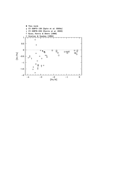
Figure 5: [Sr/Fe] as a function of [Fe/H]. Downward arrows refer to upper limits.

While Barium can also be synthesised via the $r$-process, Strontium and Yttrium are thought to be synthesised solely via the “slow neutron-capture” process ($s$-process). This process is thought to take place inside AGB stars, and given the secondary nature of the process (iron-group elements need to be pre-existing in the AGB), it starts enriching the Galaxy at later times than the products of massive SN II. Indeed, at very low metallicities, all $s$-process elements decline rapidly. However, at metallicities lower than $-$2.5, the [Sr/Fe] ratio becomes extremely scattered (see Fig. 5), by a factor almost 200. This large scatter is not found in other elements that can be produced by the $s$-process: for example, no Ba-rich dwarf star ([Ba/Fe] significantly larger than the average trend) has ever been detected in low-metallicity stars, whereas Sr-rich objects are detected (see e.g. the review by Ryan 2000). The process at work is not yet elucidated: The weak $s$-process in $\sim 15\,M_{\sun}$ stars favors low-atomic number neutron-capture species (Prantzos et al. 1990) and would thus produce Sr without much of Ba, but neutron sources at low metallicities would vanish and make the process inefficient; a low neutron-exposure $r$-process (Ishimaru and Wanajo 2000) could be at work, but both theoretical grounds and observational clues are lacking to conclude on this topic.

Our program stars happen to sample this scatter in the [Sr/Fe] ratio, HE 1303–2708 belonging to the Sr-normal group, and HE 1353–2735 to the Sr-poor. It is interesting to note that HE 1353–2735 is not the only Sr-poor star which is in a binary system: CS 22873-139 is a 19 days period extremely metal-poor binary with [Sr/Fe]$<-$1.1 (Spite et al. 2000a), and CS 22876-032 (period 427 days) is the most metal-poor dwarf known to date, with [Sr/Fe]$<-$0.65 (Norris et al. 2000).

Figure 6: Lithium 6708  Å line in the spectra of the two stars (dots). The straight lines are models with A(Li)=1.96, 2.06 and 2.16 for HE 1353–2735, and A(Li)=2.15 for HE 1303–2708. The spectrum of HE 1303–2708 was shifted vertically by $-$0.2 for the sake of clarity.

5.4 Lithium

In connection to the much debated primordial lithium abundance, and its relation to the observed lithium abundance in metal-poor dwarfs (the so-called Spite-plateau), we checked the status of this element in our two program stars. We determined the abundance from the Li I 6708 Å doublet by comparing it to synthetic spectra. Using the stellar parameters listed in Table 5, we obtain A(Li)=2.15$\pm$0.05 and 2.06$\pm$0.1 dex for HE 1303–2708 and HE 1353–2735, respectively (see Fig. 6). The uncertainties refer to the determination of the abundance itself, but do not include the uncertainty arising from the choice of stellar parameters. In particular, the Lithium abundance is very sensitive to effective temperature. We recall that we used Balmer lines to determine T${}_{\mbox{\scriptsize eff}}$, so that the present results should be compared only with data making use of the same T${}_{\mbox{\scriptsize eff}}$ scale. For this purpose, we plotted in Fig. 7 only data which used effective temperatures determined from Balmer lines (see caption for details of sources). As one can judge from the plot, both of our two stars are very close to the average value of A(Li) for their metallicity.

Figure 7: The Lithium-plateau for metal poor dwarfs hotter than 5900 K. The compilation is based on Spite et al. (1996), complemented by Spite et al. (2000b) for the most metal-poor stars, using the same temperature scale (based on H$\alpha$ wings). Also plotted are the two extremely metal-poor binaries CS 22876-032 (Norris et al. 2000) and CS 22873-139 (Spite et al. 2000a).

6 Conclusions

We presented the first abundance analysis of metal-poor stars from the Hamburg/ESO survey, based on high resolution spectra obtained with UVES at VLT-UT2. With HE 1353–2735, another Sr-rich, extremely metal-poor binary was discovered.

The very good agreement of the stellar parameters deduced from moderate-resolution, but good quality ($S/N>50$) spectra with the parameters derived from UVES spectra shows that the investment of considerable amounts of observing time at 4 m class telescopes pays off: reliably determined stellar parameters ensure that no time is wasted at 8 m class telescopes by observing uninteresting objects.

From our investigation it is evident that much larger samples of extremely metal-poor stars have to be analysed at high spectral resolution in order to decipher the chemical history of our galaxy. With UVES at VLT-UT2 now being in operation, this aim has become reachable. Fortunately there will be no lack of metal-poor targets to be observed, since in the HES, hundreds of stars at $\mbox{[Fe/H]}<-3.0$ are expected to be discovered, provided moderate-resolution follow-up spectroscopy can be obtained for all candidates.