EROS 2 PROPER MOTION SURVEY FOR HALO WHITE DWARFS

Since 1996 EROS 2 has surveyed $440^{\circ 2}$ at high Galactic latitude to search for high proper motion stars in the Solar neighbourhood. We present here the analysis of $250^{\circ 2}$ for which we have three years of data. No object with halo-like kinematics has been detected. Using a detailed Monte-Carlo simulation of the observations, we calculate our detection efficiency for this kind of object and place constraints on their contribution to various halo models. If 14 Gyr old, the halo cannot be made of more than 18% of hydrogen white dwarfs (95% C.L.).

1 Introduction

Cool white dwarfs (WDs) have become a very popular subject in the recent years, since the Macho $\!{}^{{\bf?}}$ results suggested that they contribute to the halo introduced to explain the Galactic rotation curve. Recent atmosphere models $\!{}^{{\bf?}}$ taking into account collision induced absorption predict the hydrogen WDs to be bluer than earlier, reducing the previous constraints from colour- and infrared surveys. Such blue cool WDs have recently been discovered $\!{}^{{\bf?}}$.

On the other hand, the Eros collaboration $\!{}^{{\bf?}}$ lowered its limit on the microlensing optical depth towards the Magellanic Clouds. A large number of population III WDs in the halo would also contradict some of our current ideas: the strange IMF of their progenitors, metal and Helium enrichment of the Galaxy, extragalactic observations of young haloes and observations of multi-TeV gamma rays $\!{}^{{\bf?}}$. Hence the question remains to know what the Macho lenses are. Cool WDs will also teach us about the early stages of star formation in the Galaxy and its age, and any WD older than those known today would bring important informations.

Proper motion surveys are a way to distinguish cool WDs from the more numerous, brighter and more distant disk stars by means of their much higher proper motion. Thus, EROS started a large survey, and we report the results here. We first describe the data we used and the way the high proper motion catalogue was created; then we present the current results of the EROS 2 survey about the contribution of cool hydrogen white dwarfs to the halo.

2 Description of the Survey

2.1 The Data

We used the Eros 2 wide field imager, located at La Silla Observatory, Chile. The instrument takes two $1^{\circ 2}$, $8k\times 4k$ CCD images simultaneously in two broad band filters, a visible band, between $V$ and $R$, and a red band close to $I$. Observations for the proper motion survey are conducted nearly all year round, during dark time, close to the meridian to reduce atmospheric refraction. Exposure time varies between 5 and 10 minutes, with limiting magnitudes of           $V\simeq\,21.5$ in the visible band and $I\simeq\,20.5$ in the red band. The pixel size is 0.”6.

Since 1996 we have taken 3,600 images of 442 fields located at high Galactic latitudes, mostly at 22.5h$<\alpha<3.5$h and $\delta=-39^{\circ},-45^{\circ}$ (South Galactic Pole fields), and at 10h$<\alpha<14.4$h and $\delta=-6^{\circ},-12^{\circ}$ (North Galactic Hemisphere fields). In this paper we use data taken between 1996 and 1999, for $250^{\circ 2}$ for which we have three epochs, separated by one year. The remaining fields will be analyzed when we get a third epoch.

2.2 The Reduction

The flat-fielding and debiasing were performed using the Eros package Peida. The astrometric reduction was done by fitting a two dimensional Gaussian on the objects detected by correlation with a Gaussian PSF. The parameters of the fit were used in order to remove non-stellar objects (bad pixels, cosmic rays and the largest galaxies). The images were then geometrically aligned over $11\,$arcmin chunks, using the bright stars of the field, as galaxies are not numerous enough nor well measured. Then the stars were matched with a search radius corresponding to a maximum proper motion of $6^{\prime\prime}/$yr, requiring that the fluxes be compatible within $4\sigma$. We produce this way multi-epoch catalogues in two bands.

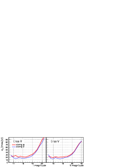
Errors were described by photon statistics and by the dispersion of bright star positions. The first contribution dominates for the faint stars, in which we expect most of our halo candidates. The second is due to the optical deformation of the (wide-field, focal reduced) telescope and the proper motion of the stars used to determine our reference frame. Total errors on a single frame range from 30 mas for bright objects, up to 150 mas at the detection limit. The external errors on the proper motion measurements are presented in Fig.1.

Figure 1: Proper motion dispersion for Eros R and Eros V images, along $\alpha$ (thick lines) and $\delta$ (thin lines).

2.3 The Selection Criteria

To eliminate the usual contamination by asteroids, noise detection, remaining cosmic rays and galaxies, we require three detections, among a set of 3 to 8 images, over three years. We then impose that the confidence level of the proper motion fit along $\alpha$ and $\delta$ be higher than 0.5%. At this point, depending on the population we want to select, we apply different sets of cuts:

$\bullet$ slow populations: objects from the disk are intrinsically slow, with a velocity dispersion of $\sigma\simeq\,20-50\,km/s$ depending on the age of the stars. At a distance of 100 pc, this translates to a proper motion of $\mu=\frac{V_{\bot}\;(km/s)}{4.74\,D\;(pc)}\approx\,80\,$mas/yr which is only a $\sim\,2-\sigma$ detection even for bright stars. This means that no proper motion will be measurable for faint stars over our small time baseline, except for the fastest or closest ones (see  3.1 for an example), and that a cross-selection between the two band catalogues will be needed, to remove noise contamination (bicolour analysis). Thus we require that the proper motion be higher than $60\,$mas/yr and $3.5\sigma$, and that the visible and red directions of proper motion be within $40^{\circ}$. This selects stars brighter than 18, as fainter stars have too large proper motion errors to be selected.

$\bullet$ halo: here we expect proper motions of 1”/yr or more, which makes any detection very significant, even with one single band (monochrome analysis), and intrinsically faint stars of $M_{V(I)}>16(15)$. Thus to remove the slower, brighter known stars we require that the reduced proper motion (RPM) $H_{V}=M_{V}+5log(V_{\bot})-3.378=V+5log(\mu)+5$, where $V_{\bot}$ is the transerve velocity in km/s, be higher than 21 in the visible band, and $H_{I}>20$ in the red band. Any star with $V>16$ or $I>15$ and $V_{\bot}>50$km/s will satisfy this cut. Additionally, as a $V=21$ disk star may have a 3–$\sigma_{\mu}$ spurious proper motion of 0.4”/yr and a misleading $H_{V}=24$, we also require the proper motion be higher than 0.7”/yr, or 200 km/s at 60 pc. This cut removes between 30% ($M_{V}=16.5$, co-rotation of 50 km/s) and 10% ($M_{V}=18$, no rotation) of detectable halo stars.

3 Results

3.1 Candidates of known Populations

Following the steps described above we select 1,046 objects in the visible band and 1,079 in the red one. Careful examination of these objects reveal that the sample is not free from contamination by spurious detections. Most candidates have a reduced proper motion $H_{V}$ between 17 and 22. Objects bluer than $V-I\simeq\,1.2$ can be interpreted mainly as thin and thick disks white dwarfs, and redder objects as disks red dwarfs. Some candidates with higher reduced proper motion, which may be spheroid objects or nearby, very cool dwarfs have been followed up spectroscopically. Denis $\!{}^{{\bf?}}$ photometry has been checked for the reddest candidates. For example, Lhs102b $\!{}^{{\bf?}}$ was first detected as a high proper motion star, then associated with Lhs102 through their common proper motion $\!{}^{{\bf?}}$, and finally confirmed as a L–dwarf by Denis and spectroscopy.

Figure 2: Distribution of detected (thick line) and expected (thin line) bright ($14<I<16.6$) bicolour candidates, for the red band. Expectations from a Besançon simulation of the Galaxy, corrected for our detection efficiency. a) Proper motion distribution. b) Proper motion direction distribution in our South Galactic Pole fields (top) and our Northern Galactic Hemisphere fields (bottom).

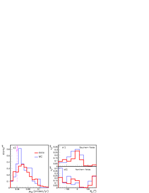
On a statistical point of view, we might check whether we reproduce well our efficiencies and our errors by comparing the thin and thick disks’ and spheroid prediction with our data set. For this we use the Besançon model of the Galaxy $\!{}^{{\bf?}}$ to create artificial catalogues of stars in our fields, then simulate the observations for these stars, using the actual distribution of each field (atmospheric conditions, number of exposures,…). We compare star counts, which indicate compatibility between the data and the Monte-Carlo for bright stars, at the 15% level. For faint objects the stars are dominated by galaxies and detailed comparison is impossible until we get a better classification of our objects. We can then apply to the resulting simulated data the slow populations set of cuts to check our sensitivity to small proper motions. We observe in Fig.2a that the results agree with the model within 20%. As we lack detailed explanation for the difference, we conservatively lower our sensivity by 20%. We also checked that our proper motion direction distribution, which mainly depends on the Sun own peculiar motion, agrees well with the Besançon distribution (see Fig.2b).

3.2 Constraints on the Halo

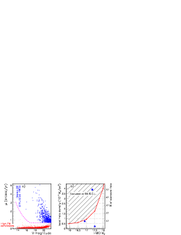
As with the known populations simulation, we simulated various kinds of haloes made of old hydrogen white dwarfs, with different HWD ages, masses and kinematics. The luminosity function of HWDs and the colour–magnitude function are those of Chabrier $\!{}^{{\bf?}}$ and Saumon & Jacobson $\!{}^{{\bf?}}$. We also indicate our sensitivity to haloes with Dirac-like luminosity functions (see Table 1). The detailed distribution of magnitudes is not crucial as only the stars in the brighter part of the luminosity function ($M_{V}=17.2\pm 0.2$ for a 14 Gyr halo, $M_{V}\approx 17.8\pm 0.3$ for 15 Gyr) contribute. Colour is important as a $V-I<0.5$ WD will be easily missed in the red band, or a $V-I>1.5$ in the visible, but this effect is compensated in our survey by the independent use of the two filters. Finally the cooling curve evolves with the WD mass; $1.2M_{\odot}$ WDs cool faster than $0.6M_{\odot}$ ones $\!{}^{{\bf?}}$. One should also remember that we measure a local number density rather than a mass density. The kinematics used correspond to the usual sets of parameters observed for the spheroid and expected for the halo, with a small rotation $-50<\omega<50$ km/s and velocity dispersion of 150–250 km/s. This is not crucial as most of the nearby HWDs in any model will have a proper motion above the 0.7”/yr cut. Conservatively we apply the correction for our sensitivity mentioned above, although it concerns the bicolour search for small proper motions, while we search here for large proper motion in each band independently. An example of a simulation is shown Fig.3a.

We find no halo type candidates in any band. Given our expectations of Table 1, we exclude a local number density higher than $2.3\,10^{-3}\,$WD$/pc^{3}$ of 14 Gyr HWDs at the 95% C.L. The exclusion diagram, as a function of the halo WD $M_{V}$ magnitude, is shown in Fig.3b.

Table 1: Expectation and constraints for HWDs of a certain $M_{V}$ magnitude, and for different halo ages. Density limit at 95% C.L. For the expectation and mass density figures, we assumed a local density of $7.8\,10^{-3}M_{\odot}/pc^{3}$, for $0.6M_{\odot}$ HWDs. Figures in the left column are for the red band, in the right band for the visible band.

	$M_{V}$ magnitude of HWDs						Halo age (Gyr)
	16.5		17		17.5		14		15
explored vol.	2.5	2.9	1.5	1.9	0.5	1.0	0.9	1.3	-	0.3	1000 pc3
expectation	33.1	37.6	19.2	25.1	6.7	13.3	11.4	17.2	0.7	3.6	WDs
star density	1.2	1.0	2.0	1.6	5.8	2.9	3.4	2.3	-	11	$10^{-3}\,$WD/$pc^{3}$
mass density	0.7	0.6	1.2	0.9	3.5	1.8	2.0	1.4	-	6.6	$10^{-3}\,M_{\odot}/pc^{3}$

Figure 3: a) Proper motion vs. $V$ for high PM monochrome candidates (dots) and simulated $M_{V}=17$, $0.6M_{\odot}$ HWDs passing the cuts (statistics $\times 20$, circles), for the visible band. The halo PM cut is indicated by the dashed line. b) Exclusion diagram as a function of the halo WD $M_{V}$ magnitude, for $0.6M_{\odot}$ HWDs. The WD halo fraction central values suggested by Ibata et al$\,{}^{8}$ (square), Ibata et al$\,{}^{9}$ (triangle), Flynn et al$\,{}^{5}$ (star) are indicated.

4 Conclusion

Using the first three years of data for 282 EROS 2 fields, we can place an upper limit of 18% (95% C.L.) to the contribution of white dwarfs of age 14 Gyr or of magnitude $M_{V}=17.2$. We are compatible with the EROS microlensing results towards the Magellanic Clouds $\!{}^{{\bf?}}$ and the analysis of proper motion observations by Flynn & al $\!{}^{{\bf?}}$ and Ibata & al $\!{}^{{\bf?}}$. We exclude a 50% contribution by $M_{V}\approx 17$ HWDs suggested by Ibata & al $\!{}^{{\bf?}}$ or Mendez & al $\!{}^{{\bf?}}$, whose blue point-like objects remain to be identified. We do not place constraints on fainter objects, either older or with a pure-helium atmosphere. In the coming months additional data will become available, so that more fields will be analyzed in addition to those presented here.

Note: During the talk in Les Arcs we presented the results of the bicolour halo analysis. Since then we progressed on the more sensitive, monochrome halo analysis, which is presented here.

References

- [1] C. Alcock et al, ApJ 479, 119 (1997) and astro-ph/0001272.
- [2] G. Chabrier, ApJ 513, L103 (1999).
- [3] G. Chabrier et al, accepted by ApJ, astro-ph/0006363.
- [4] X. Delfosse et al, A&AS 135, 41 (1999).
- [5] Ch. Flynn et al, MNRAS, astro-ph/9912264 (2000).
- [6] B. Goldman et al, A&A 351, L5 (1999).
- [7] D. S. Graff et al, ApJ 523, L77 (1999).
- [8] R. A. Ibata et al, ApJ 524, L95 (1999).
- [9] R. A. Ibata et al, ApJ 532, L41 (2000).
- [10] T. Lasserre et al, A&A 355, L39 (2000).
- [11] R. A. Méndez and D. Minniti, ApJ 529, 911 (2000).
- [12] A. Robin and M. Crézé, A&A 157, 71 (1986) and http://www.obs-besancon.fr/www/modele/modele.html.
- [13] D. Saumon and S. B. Jacobson, ApJ 511, L107 (1999).
- [14] W. F. van Altena, J. T. Lee, E. D. Hoffleit, The General Catalogue of Trigonometric Stellar Parallaxes, Fourth Edition, (Yale University Observatory, 1995).