The local space density of Sb-Sdm galaxies as function of their scalesize, surface brightness and luminosity

Abstract

We investigate the dependence of the local space density of spiral galaxies on luminosity, scalesize and surface brightness. We derive bivariate space density distributions in these quantities from a sample of about 1000 Sb-Sdm spiral galaxies, corrected for selection effects in luminosity and surface brightness. The structural parameters of the galaxies were corrected for internal extinction using a description depending on galaxy surface brightness. We find that the bivariate space density distribution of spiral galaxies in the (luminosity, scalesize)-plane is well described by a Schechter luminosity function in the luminosity dimension and a log-normal scale size distribution at a given luminosity. This parameterization of the scalesize distribution was motivated by a simple model for the formation of disks within dark matter halos, with halos acquiring their angular momenta through tidal torques from neighboring objects, and the disk specific angular momentum being proportional to that of the parent halo. However, the fractional width of the scalesize distribution at a given luminosity is narrower than what one would expect from using the distribution of angular momenta of halos measured in N-body simulations of hierarchical clustering. We present several possible explanations for the narrowness of the observed distribution. Using our bivariate distribution, we find that determinations of the local luminosity function of spiral galaxies should not be strongly affected by the bias against low surface brightness galaxies, even when the galaxies are selected from photographic plates. This may not be true for studies at high redshift, where (1+z)⁴ surface brightness dimming would cause a significant selection bias against lower surface brightness galaxies, if the galaxy population did not evolve with redshift.

Accepted for publication in the Astrophysical Journal

1 INTRODUCTION

In the last few decades, many papers have been devoted to the measurement of the luminosity function (LF) of galaxies, of their distribution of central surface brightnesses and, to a lesser extent, of their distribution of scalesizes. The observational determinations of these three types of distribution cannot in practice be separated, because of the limitations of the surveys on which the investigations are based. Any galaxy LF is only valid to the surface brightness limit of the survey from which it is derived, while any distribution of surface brightnesses is valid only over some range in luminosity or scalesize, depending on the survey limits in apparent magnitude and/or angular size. In this paper we address this problem directly, by investigating the bivariate distribution functions of spiral galaxies in combinations of luminosity, surface brightness and scale size. Knowledge of any two of these quantities then suffices to determine the third.

Bivariate distribution functions have two important applications. First of all, bivariate distribution functions are the only proper way to compare samples with different selection criteria, especially when comparing samples at different redshifts. For instance, comparing LFs determined from samples with similar magnitude limits but different lower surface brightness limits will result in discrepancies in the magnitude range where the contribution from low surface brightness galaxies is significant. Secondly, bivariate distribution functions provide excellent tests for galaxy formation and evolution theories. Any complete galaxy formation theory should be able to explain the distribution functions of galaxy structural parameters. Obviously, the 2-dimensional (2D) distribution functions provide more constraints on formation theories than the separate 1D distributions of surface brightness, scalesize and luminosity obtained by integrating over the other quantity in the bivariate distribution.

As already mentioned, every optically-selected galaxy sample always has limits in surface brightness in addition to its limits in apparent luminosity and/or angular diameter. The detection volume (or visibility) for a particular type of galaxy in a such a survey is then at least a two-parameter function, e.g. of luminosity and scalesize, and depends strongly on these parameters, resulting in strong biases against low surface brightness (LSB) and small scalesize galaxies (Disney & Phillipps 1983; Allen & Shu 1979; McGaugh, Bothun & Schombert 1995). Since the determination of the space density of galaxies from a survey depends on knowing the detection volumes, the only complete description of the galaxy space density which can be obtained observationally is a bivariate distribution function which includes two of the three parameters of surface brightness, scalesize and luminosity. To study the bivariate distribution of field spiral galaxies, it is straightforward to show that one has to obtain surface photometry and distances of at least 500-1000 galaxies, in order to avoid problems with small number statistics near the selection boundaries (de Jong & Lacey 1999).

Because of the large number of galaxies needed with both redshifts and good surface photometry, determinations of bivariate distribution functions of spiral galaxies as functions of structural parameters have been relatively rare. Some notable exceptions are Phillipps & Disney (1986), who presented a (magnitude, surface brightness)-distribution of Virgo spiral galaxies using RC2 data, van der Kruit (1987), who used a diameter-limited sample of 51 galaxies to construct a crude (surface brightness, scale length)-distribution, and Sodrè & Lahav (1993) who created a (magnitude, diameter)-diagram from the ESO-LV catalog. More recently Lilly et al. (1998) used the CFRS redshift survey to derive the bivariate function in the (magnitude, scalesize)-plane, and made a first attempt at studying its redshift evolution. Finally, Driver (1999) used a volume-limited selection of galaxies in the Hubble Deep Field (Williams et al. 1996) to probe the really low surface brightness regime of the bivariate distribution function. The results of nearly all of these studies suffered from small number statistics, and very few firm physical conclusions could be drawn.

Theoretical predictions for the sizes of galaxy disks in the hierarchical clustering picture of galaxy formation began with the classic paper by Fall & Efstathiou (1980). They considered the formation of a disk by the collapse of gas within a gravitationally dominant dark matter (DM) halo. They showed how the radius of the disk is related to that of the halo, on the assumption that the gas starts off with the same specific angular momentum as the dark matter, and conserves its angular momentum during the collapse. Thus in this picture, the disk radius depends on the amount of angular momentum which the halo acquires prior to collapse through the action of tidal torques from neighboring objects. This model naturally leads to typical disk sizes similar to those observed for bright spiral galaxies. Many authors have subsequently made calculations of disk sizes within the same basic framework (see e.g. van der Kruit 1987; Mo et al. 1998; van den Bosch 1998), and Dalcanton et al. 1997b combined this model with a Schechter luminosity function for galaxies to predict the bivariate distribution of surface brightness and scale length for disks. We will parameterize our observed bivariate distribution function for disks in a way that is motivated by this same simple model.

More recently, predictions for galaxy properties in hierarchical clustering models have been developed much further using the technique of semi-analytic modeling (Cole et al. 1994, 2000; Kauffmann, White & Guiderdoni 1993, Somerville & Primack 1999). The semi-analytic models include much more of the physics of galaxy formation, including the merging histories of DM halos, gas cooling and collapse within halos, star formation from cold gas, feedback from supernovae, and the luminosity evolution of stellar populations. In this paper we will compare the observed bivariate distribution function with the most recent semi-analytic model predictions from Cole et al. (2000).

This paper is organized as follows. In §2 we describe how one can correct a sample of objects for distance dependent selection effects. In §3 we describe the sample we have used for this investigation and how we determine physical quantities from the observations. In §4 we determine the bivariate distributions of space density and luminosity density for the local universe. We propose a model for the bivariate distribution functions based on the hierarchical galaxy formation scenario and fit this model to the data in §5. Finally, we discuss the results in §6 and summarize our conclusions in §7.

2 VISIBILITY CORRECTION

The use of selection criteria to define a sample of objects often introduces selection biases, even in so called “complete samples”, i.e. samples that are complete according to their selection criteria. Malmquist (1920) was one of the first to quantify the bias in the determination of the average absolute magnitude of a stellar sample due to the real spread in luminosity combined with the distance-dependent selection limit that results from applying a cut-off in apparent magnitude. The uncertainty in the measurement of the selection magnitude introduces another bias near the selection limit, which can be described in the same way as Malmquist’s original bias if the uncertainties have a Gaussian error distribution. Both of these effects (which are mathematically similar in case of Gaussian luminosity and error distributions, but have completely different origins) have been called Malmquist bias by different authors. To make matters even more confusing, the biases in distance measurements resulting from the use of samples suffering from these effects have also been called Malmquist bias.

In this section we describe how to correct a sample for distance-dependent biases and for biases resulting from uncertainties in the selection parameters. We pay particular attention to the case where the sample has been selected on angular diameters.

2.1 Volume Correction

Our aim is to determine the average space density of galaxies with certain properties in the local universe. Most field galaxy samples are not based on distance- or volume-limited surveys, but are limited by some quantity more readily available observationally, like apparent magnitude or angular diameter. Not all galaxies have the same luminosity or physical diameter, and therefore they can be seen to different distances before dropping out due to the selection limits. The volume within which a galaxy can be seen and will be included in the sample ($V_{\rm max}$) goes as the distance limit cubed, which results in galaxy samples being dominated by intrinsically bright and/or large galaxies, because these have the largest visibility volume (Disney & Phillipps 1983; McGaugh et al. 1995).

In this paper we use one of the simplest methods available for correcting for selection effects, the $V_{\rm max}$ correction method (Schmidt 1968). Each galaxy is given a weight equal to the inverse of its maximum visibility volume set by the selection limits (a formal derivation can be found in Felten (1976)). For a low redshift sample with upper ($D_{\rm max}$) and lower ($D_{\rm min}$) limits on the major axis angular diameter, this leads to

$$V_{\rm max}=\Omega_{f}\frac{4\pi}{3}d^{3}\left[\left(\frac{D_{\rm maj}}{D_{\rm max}}\right)^{3}-\left(\frac{D_{\rm maj}}{D_{\rm min}}\right)^{3}\right]$$ (1)

with $\Omega_{f}$ the fraction of the sky used to select the galaxies, $d$ the distance to the galaxy, and $D_{\rm maj}$ the major axis angular diameter of the galaxy. Other limits, like redshift or magnitude limits, that would limit $V_{\rm max}$ can trivially be taken into account as well. For higher redshift samples we have to take cosmological corrections into account. We define the bivariate density distribution $\phi(x,y)$ in parameters $x$ and $y$ such that $\phi(x,y)\,dx\,dy$ is the number density of galaxies in the interval $(x,y),(x+dx,y+dy)$. For a sample of $N$ galaxies which is complete to within the selection limits, we can now define an estimator of this quantity as follows:

$$\phi(x,y)\approx\frac{1}{\Delta x\Delta y}\sum_{i}^{N}\frac{\delta^{i}}{V_{\rm max}^{i}},$$ (2)

where $i$ is summed over all galaxies, and $\delta^{i}=1$ if the ($x_{i}$,$y_{i}$) parameters of galaxy $i$ are in the bin range ($x\pm\Delta x/2,y\pm\Delta y/2$), and 0 otherwise.

The $V_{\rm max}$ correction method assumes a uniform distribution of galaxies in space, and is not unbiased against density fluctuations. To give unbiased results, objects with the smallest $V_{\rm max}$ in the sample should be visible on scales larger than the largest scale structure. Currently, such samples do not exist. Other methods exist that take density fluctuations into account (for reviews see e.g. Efstathiou et al. 1988; Willmer 1997). These methods assume a direct relation between the distribution parameter and the selection parameter. This is not the case in the current investigation (selection on $B$-band diameters versus distributions of $I$-band magnitudes, surface brightnesses and scalesizes).

The $V_{\rm max}$ corrections of equations (1) and (2) are valid only if similar galaxies have their angular diameters measured at the same physical diameter, independent of distance (see the discussion in de Jong 1996b). It is not important if a particular class of galaxies has their diameters measured at an intrinsically larger physical diameter compared to other classes (for instance, at a lower surface brightness). This class of galaxies will be over-represented in the sample, but on average will have a larger distance, so that the effects exactly cancel out in the estimator (2), as they are designed to do. In a similar fashion to de Jong & van der Kruit (1994), we determined that the ratio of eye-estimated to isophotal diameters was independent of diameter, and we therefore conclude that most likely the diameters of all similar galaxies were measured at the same physical (linear) diameter.

The uncertainty in the $\phi(x,y)$ estimator of equation (2) is in general dominated by Poisson statistics: what is the uncertainty on the mean number of galaxies in a bin, if $N$ are detected? It is easy to show that at least 500 galaxies with accurate photometry and distances are needed to determine a bivariate distribution function of structural parameters (de Jong & Lacey 1999). Only if we have many galaxies in a bin is the error in $\phi(x,y)$ no longer dominated by Poisson statistics, but becomes dominated by the uncertainty in $V_{\rm max}$. The uncertainty in $V_{\rm max}$ in equation (1) arises from galaxy distance uncertainties and diameter uncertainties. The distance uncertainty of each galaxy ($\sigma^{i}_{d}$) contributes a component $\sum_{i}^{N}(\frac{\sigma^{i}_{d}}{d^{i}}\frac{3\delta^{i}}{V_{\rm max}^{i}})^{2}$ to the variance in the determination of $\phi(x,y)$. The diameter uncertainties ($\sigma^{i}_{D_{\rm maj}}$) add a $\sum_{i}^{N}(\frac{\sigma^{i}_{D_{\rm maj}}}{D^{i}_{\rm maj}}\frac{3\delta^{i}}{V_{\rm max}^{i}})^{2}$ to the variance, but are on top of that directly related to the selection of the sample, and are further discussed in the next section.

2.2 Selection Uncertainty Correction

The parameters used to select the galaxy sample can only be determined with finite accuracy. The selection parameters have to be distance dependent for $V_{\rm max}$ corrections to be used, leading to what often is called the Malmquist edge bias. Assuming a symmetric error distribution on the selection parameters (e.g. diameter or magnitude), objects at the selection limit have an equal probability of being scattered into the sample as being scattered out of the sample. Because there are more small and faint than large and bright objects on the sky (due to the effect described in the previous paragraph), on average more objects are scattered into the sample than than out of the sample, and we will overestimate the number of objects in our search volume.

Once we have determined the probability distribution of the error in the selection parameters ($P(x)$), we can correct the $V_{\rm max}$ method for this edge bias. We might try to correct for the bias by taking the average 1/$V_{\rm max}$ weighted with the error distribution of the selection parameters within the selection limits. Unfortunately, this procedure would result in an overcorrection. An object at the selection limit would count for only half (with the other half being outside the selection limits assuming a symmetrical error distribution), but an object just outside the selection limit with a large fraction of its probability function within the limits would not be included at all. To remedy this effect, we take a virtual selection limit $t\sigma$ away from the original selection limit and now include the objects between the virtual and original selection limits with appropriate (low) weight.

Figure 1: Observed diameters versus the probability distributions of true diameters for three galaxies. The solid diagonal line is the line of equality, the dashed and dotted lines indicate different minimum diameter selection limits in observed and true angular diameters. For detailed explanation see text.

We demonstrate this for the case of diameter selection with the use of Fig. 1, where we plot three galaxies of different observed diameters $D_{\rm maj}$. Galaxy A has an observed diameter just below the selection limit $D_{\rm min}$ (indicated by the vertical dashed line), galaxy B is at the selection limit and galaxy C has an observed diameter slightly larger than the selection limit. Each galaxy has an associated probability distribution of true diameter $D_{\rm true}$, indicated by the Gaussian distributions. We can calculate a corrected 1/$V_{\rm max}$ for each galaxy using equation (1), averaged over the range of true diameters for each galaxy, weighted appropriately for the true diameter probability. If we take the true diameter cut-off the same as the observed diameter cut-off (indicated by the horizontal dashed line), than galaxy B is only counted for half a galaxy, galaxy C is counted almost completely, and galaxy A is counted for a small but significant fraction (dark and light shaded regions). We now have the situation where galaxy A should have been included, because a significant part of its true diameter distribution is larger than the true diameter selection limit, but the galaxy is in fact not included in the sample at all because its observed diameter is below the selection limit. This attempt to correct for the edge bias is therefore wrong, as we are not counting galaxies that should have been included. But by shifting the virtual true diameter selection limit upwards (indicated by the dotted line) and calculating the $V_{\rm max}$ values from equation (1) with this shifted diameter limit, we only have to weight the galaxies for the dark shaded regions. Galaxy A has now a negligible fraction of true diameters above the true diameter selection limit, which is good because it was not in the sample to begin with. Other galaxies just above the selection limit get little weight, but have the appropriate corrected 1/$V_{\rm max}$ values.

In our example of a complete sample selected with upper and lower angular diameter cut-offs $D_{\rm max}$ and $D_{\rm min}$, we get for the corrected 1/$V_{\rm max}$to use in equation (2)

$$1/V_{\rm max}^{\rm cor}=\frac{\int_{D_{\rm min}+t\sigma}^{D_{\rm max}-t\sigma}P(D|D_{\rm maj})/V_{\rm max}(D)\,dD}{\int_{-\infty}^{\infty}P(D|D_{\rm maj})\,dD},$$ (3)

where $P(D|D_{\rm maj})$ denotes the probability of the true angular diameter of a galaxy being $D$ at a given observed angular diameter $D_{\rm maj}$, and $V_{\rm max}$(D) is to be evaluated using equation (1) with $D_{\rm min}$ replaced by $D_{\rm min}+t\sigma$ and $D_{\rm max}$ replaced by $D_{\rm max}-t\sigma$. We should try to make $t\sigma$ as large as possible, so that $P(D\pm t\sigma|D)$ is small, and the probability of a galaxy apparently being outside the selection limits but in reality belonging inside is small. Unfortunately, we cannot make $t\sigma$ too large, as then very few galaxies will remain with significant weights.

3 SAMPLE SELECTION AND DATA

We have used the galaxy sample described by Matthewson, Ford and Buchhorn (1992) and Matthewson & Ford (1996, MFB sample hereafter) as the starting point for our sample selection. The MFB data were obtained mainly to study peculiar motions using the Tully-Fisher (1977) relation. The MFB sample is nearly ideal for the kind of study we want to perform. With more than a thousand field galaxies it is large enough not to run immediately into small number statistics near the low surface brightness and/or small scalesize selection borders. Matthewson et al. collected for most objects the CCD surface photometry and redshifts required for our statistical study. The main drawback of the sample is its selection, as the sample was defined as a subsample of the ESO-Uppsala Catalog of Galaxies (Lauberts 1982), which is a catalog selected by eye from photographic plates. Unfortunately, nothing better exists at the moment, and it remains to be seen whether automated surveys like Sloan, DENIS and 2MASS will go deep enough to detect LSB galaxies. These surveys should however discover and quantify the number of galaxies with small scalesizes.

The MFB sample is not entirely complete, as some selected galaxies had to be excluded due to too bright foreground stars, too disturbed morphologies to obtain reliable surface brightness profiles or inability to obtain redshifts. As incompleteness is an issue in our analysis, we went back to ESO-Uppsala catalog and reselected galaxies using selection criteria close to the MFB sample criteria. Our criteria are: ESO-Uppsala diameter $1.65\arcmin$ $\leq$ $D_{\rm maj}$ $\leq$ $5.05\arcmin$, galactic latitude $|b|>11\arcdeg$, morphological type $3$ $\leq$T$\leq$ $8$ and minor-over-major axis ratio $0.1736$ $<$ $D_{\rm min}/D_{\rm maj}$ $<$ $0.776$. This last criterion is different from MFB, excluding the edge-on galaxies for which extinction corrections are large and uncertain. These selection criteria resulted in a sample of 1007 galaxies, with a subsample of 818 galaxies (81.2%) for which we have both MFB surface photometry and redshifts (some redshifts were obtained from the NED and LEDA databases).

A $V/V_{\rm max}$-test (Schmidt 1968; see also de Jong 1996b) corrected for Malmquist edge bias showed that the sample has an average $V/V_{\rm max}$ of 0.507$\pm$0.010 and is therefore statistically complete. A slight incompleteness for high surface brightness galaxies ($\langle V/V_{\rm max}\rangle=0.454\pm 0.021$ for galaxies with $\mu_{\rm 0}$ $<$ $19$ $I$-mag arcsec^-2) was detected. This means we have either too many high surface brightness galaxies nearby or too few at large distance. We could find no obvious reason why this might be the case. For the lower surface brightness bins the $V/V_{\rm max}$ indicated statistical completeness.

Accurate distances are essential to calculate the $V_{\rm max}$ corrections. Applying blind Hubble flow distances would introduce large errors for many of the smallest, nearby galaxies. Luckily, because the MFB sample data were obtained to measure peculiar motions, many of our galaxies have Tully-Fisher distances (Tully & Fisher 1977). For the 706 galaxies in our sample also included in the Mark III catalog (Willick et al. 1997) we used group velocities for groups with recession velocities larger than 2000 km/s, otherwise the Mark III Malmquist bias corrected velocities. For galaxies not included in the Mark III catalog, we used their Heliocentric velocity corrected to the Local Group velocity according to the precepts of Karachentsev & Makarov (1996). All these velocities were converted to distances using a Hubble constant of 65 km s^-1 Mpc^-1. When calculating the $V_{\rm max}$ corrections, we assume a 15% distance error for the galaxies with Mark III velocities and a 250 km/s peculiar velocity uncertainty for the remaining galaxies (1 sigma uncertainties).

Twenty percent of the galaxies have velocities of less than 2000 km/s and about another 20% have velocities exceeding 5000 km/s. For the brightest galaxies we therefore sample large enough scales not to be influenced by large scale density fluctuations, but for smaller galaxies this may not be the case. However, because $V/V_{\rm max}$-tests indicated completeness and homogeneity of the sample independent of surface brightness and scalesize, we are not overly concerned by this.

We calculated the characteristic global structural parameters of the galaxies from the radial $I$-band luminosity profiles. MFB calculated luminosity profiles by determining the average surface brightness on elliptical annuli, which had been fitted to the galaxy isophotes. The total luminosity ($M_{I}$) of the galaxies was calculated by extrapolating the last few measured points of the profiles to infinity with an exponential luminosity profile. This luminosity was used to calculate the effective (half total enclosed light) radius ($r_{\rm e}$). The average surface brightness within the effective radius –which we will call effective surface brightness ($\langle\mu\rangle_{\rm e}$) hereafter– was calculated using $\langle\mu\rangle_{\rm e}=M_{I}-5\log(r_{\rm e})-2.5\log(2\pi)$.

In addition to the structural parameters for the galaxy as a whole, we also use in this paper the structural parameters for the disk alone. We decomposed the 1D luminosity profiles into bulge and disk contributions, using exponential light profiles for both disk and bulge (see de Jong 1996a). This yielded the structural parameters disk magnitude ($M_{I,D}$), disk central surface brightness ($\mu_{\rm 0}$) and disk effective radius ($r_{\rm e,D}$), which equals 1.679 times the disk e-folding scale length. In agreement with de Jong (1996a), the 1D disk parameters showed good agreement with the disk parameters determined by Byun (1992), who used a 2D fitting method and an $R^{\frac{1}{4}}$ instead of exponential profile for the bulge.

The Galactic foreground extinction corrections were calculated according to the precepts of Schlegel, Finkbeiner & Davis (1998). The proper internal extinction correction for disk galaxies is still heavily in debate. Many different corrections have been proposed, resulting from a large variety of methods and galaxy samples. Here we use the method of Byun (1992), also described in detail by Giovanelli et al. (1995), to correct quantities to face-on values. Using this method, the parameter for which the extinction correction has to be determined is first fitted against the inclination corrected maximum rotation velocity of the disk ($V_{\rm rot}$). The residuals on this fit are next fitted against $\log(D_{\rm min}/D_{\rm maj}$) to empirically determine the effect of extinction as a function of inclination relative to face-on. The extra step of fitting to the residuals of the $V_{\rm rot}$ relation reduces the distance dependent selection effects as function of inclination.

In contrast to Giovanelli et al. (1995) and Tully et al. (1998), we divide the extinction measurements into several surface brightness bins instead of absolute magnitude bins, as we expect the amount of extinction to be more related to surface brightness than luminosity. If the amount of dust at a given radius in the galaxy is in some way proportional to the amount of stars at that radius (i.e. local surface brightness), then for a disk-like configuration the relative extinction as function of inclination will be determined by surface brightness, independent of scalesize and hence magnitude. Even so, because the magnitudes and surface brightnesses of galaxies are to some extend correlated, one will also see a trend between magnitude and extinction. The equations used for the extinction corrections are listed in Table 1. We find that the low surface brightness galaxies in our sample behave as nearly transparent disks, while high surface brightness disks behave as having optical depth larger than one near the center.

Table 1: Internal extinction corrections

corr. par.	equation used
$\langle\mu\rangle^{i}_{\rm e}$	$\langle\mu\rangle_{\rm e}\,+\,(0.180(\langle\mu\rangle_{\rm e}-24)-0.030)\log(D_{\rm maj}/D_{\rm min})$
$\mu^{i}_{\rm 0}$	$\mu_{\rm 0}\,+\,(0.613(\langle\mu\rangle^{i}_{\rm e}-24)+2.862)\log(D_{\rm maj}/D_{\rm min})$
$\log(r^{i}_{\rm e})$	$\log(r_{\rm e})\,-\,(0.039(\langle\mu\rangle^{i}_{\rm e}-24)+0.083)\log(D_{\rm maj}/D_{\rm min})$
$\log(r^{i}_{\rm e,D})$	$\log(r_{\rm e,D})\,+\,(0.019(\langle\mu\rangle^{i}_{\rm e}-24)+0.036)\log(D_{\rm maj}/D_{\rm min})$
$M^{i}_{I}$	$M_{I}\,+\,(0.197(\langle\mu\rangle^{i}_{\rm e}-24)-0.058)\log(D_{\rm maj}/D_{\rm min})$
$M^{i}_{I,D}$	$M_{I,D}\,+\,(0.295(\langle\mu\rangle^{i}_{\rm e}-24)-0.488)\log(D_{\rm maj}/D_{\rm min})$

Figure 2: Observed distribution of effective surface brightness versus effective radius, both corrected for extinction to face-on values. The dotted lines show the maximum indicated distances to which face-on exponential disk galaxies can be observed given the selection criteria of our sample. Different symbols are used to denote the indicate ranges of ESO-Uppsala morphological T-type.

Figure 2 shows the distribution of the galaxies as a function of the extinction-corrected values $\langle\mu\rangle^{i}_{\rm e}$ and $r^{i}_{\rm e}$. The dotted lines illustrate the selection biases for this sample. The sample should be complete to the indicated distances, for galaxies above and to the right of the lines, if we assume purely face-on exponential disks. The lines were calculated assuming the average surface brightness at $D_{\rm maj}$ is 24.83 $I$-mag arcsec^-2, as determined from the data. This diagram shows clearly the selection biases against low surface brightness and small scalesize galaxies. Only the highest surface brightness, largest scalesize galaxies can be seen out to 100 Mpc. The galaxies near the 100 Mpc line have a 125 times larger visibility volume than the galaxies near the 20 Mpc line, which makes visibility corrections essential to calculate real space density distributions from the apparent distribution in the figure.

4 SPACE DENSITY DISTRIBUTIONS

Before we can calculate the true space density of galaxies using the equations derived in §2, we have to determine the uncertainty in the diameter selection parameter. To this end, we obtained 250 $B$-band images of galaxies in the ESO-LV catalog (Lauberts & Valentijn 1989), scanned from the same photographic plates that were used to define the ESO-Uppsala catalog from which our sample was selected. One of us (RSdJ) went three times through the images, measuring the diameters with a cursor on a computer screen. These three sets of diameters were compared to the ESO-Uppsala diameters and compared to each other. It was found that the uncertainty in the diameters was more constant in the absolute than the relative sense in the range of diameters where we can be reasonably sure that we are complete (2.2′$\leq$ $D_{\rm maj}$ $\leq$4.2′). The rms error between our measurements was 0.21′, while the rms error between our diameter measurements and the ESO-Uppsala diameters was 0.31′. This difference results from the difference in measurement technique (with eye, magnifying glass and ruler versus computer screen and cursor). The ESO-Uppsala diameters were quantified to the nearest 0.1 minute of arc, while the human brain has a preference for ‘nice’ numbers. The diameter distribution of the ESO-Uppsala catalog shows distinct peaks at 2′, 2.2′, 3′, 3.5′, 4′ and 5′. If we had re-measured the ESO-Uppsala diameters in exactly the same way as was done originally, we expect that the rms difference between our own and the ESO-Uppsala measurements would have been lower than determined now, and we therefore adopt an uncertainty in the ESO-Uppsala diameters of 0.25′ to be used in equation (3).

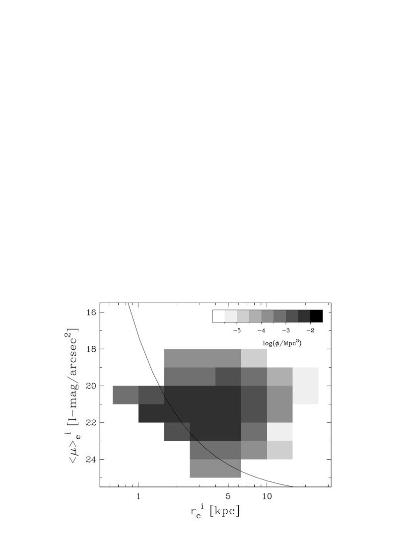
Figure 3: Bivariate space density distribution of Sb-Sdm galaxies as a function of effective surface brightness and effective radius. The line indicates the 20 Mpc sample selection limit for face-on exponential disks. To the left of the line we are limited by small number statistics and local density fluctuations.

To calculate the true space density of galaxies in the ($\langle\mu\rangle_{\rm e}$, $r_{\rm e}$)-plane, we have to weight each of the galaxies in Fig. 2 using the visibility correction equations given in §2. In Fig. 3 we show the space density of Sb-Sdm galaxies in number per Mpc³. The 20 Mpc visibility limit of face-on galaxies with exponential disks is indicated by the solid line. To the left of this line we are limited by small number statistics and local density fluctuations, but to the right we should have a reasonably fair sampling of the local universe. The limits on the distribution at the high surface brightness and large scalesize ends are therefore real. Note for instance that this distribution strongly suggests that a galaxy like Malin I (Bothun et al. 1987) with $\langle\mu\rangle^{i}_{\rm e}\simeq 26$ $I$-mag arcsec^-2 and $r_{\rm e}\simeq 140\,$kpc must be extremely rare.

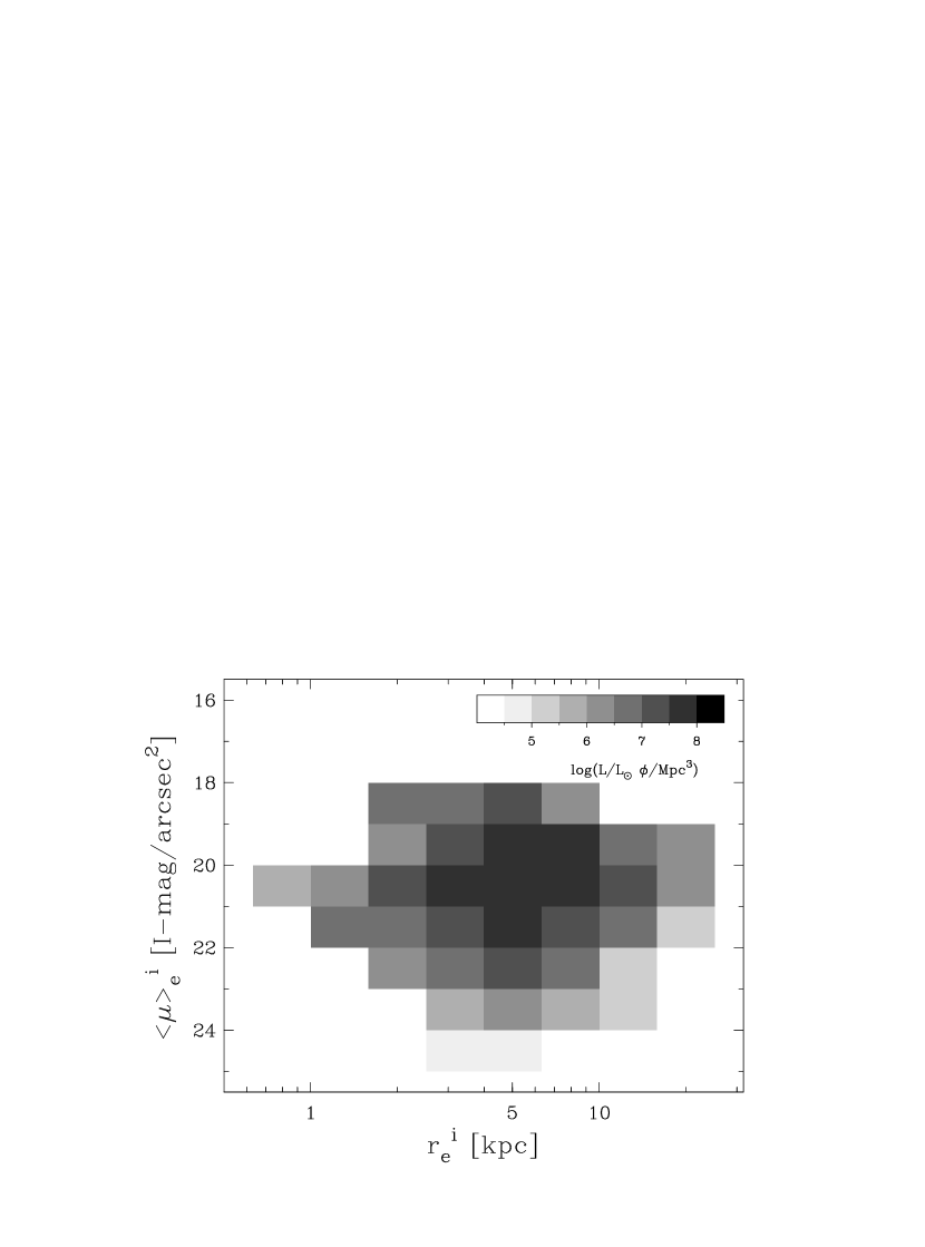
Figure 4: Bivariate luminosity density distribution of Sb-Sdm galaxies as a function of effective surface brightness and effective radius.

Perhaps even more important than the space density of galaxies is their luminosity density, which is presumably indicative of the stellar (and baryonic) mass density. Weighting each galaxy in Fig. 3 with its luminosity results in Fig. 4, where we have used $M_{\sun}=4.14$ $I$-mag to convert the $I$-band magnitudes to luminosities in solar units (Cox 2000, transfering from Johnson to Kron-Cousins $I$-band using Bessell 1979). Spiral galaxies with effective radii of order 6 kpc and $\langle\mu\rangle_{\rm e}\simeq 20$ $I$-mag arcsec^-2 provide most of the spiral galaxy luminosity in the local universe. It should come as no surprise that we live in a galaxy with these qualifications. The contribution of LSB spiral galaxies to the total luminosity density of the universe apears to be small. We will discuss this issue in more detail in §6.

5 A FUNCTIONAL FORM

In this section we will derive a functional form to describe the bivariate distributions calculated in the previous section. The parametrization of the bivariate distributions will be useful to compare distributions derived from differently selected samples and to study redshift evolution. The parametrization can also be used in modeling where both galaxy luminosity and size are required (e.g. modeling the cross-sections of galaxies for producing quasar absorption lines).

Figure 5: Bivariate space density distribution of Sb-Sdm galaxies as a function of inclination corrected effective radius in different bins of absolute $I$-band magnitude as indicated in the top-right corner of each panel. The error bars on the histogram indicate the 95% confidence limits due to Poisson statistics and distance and diameter uncertainties. The upper limits are the 95% confidence upper limits derived from non-detections assuming Poisson statistics for face-on exponential disks of the given parameters. The dashed line shows the fitted bivariate distribution function of equation (5.1) as described in the text.

In the previous sections we used the distributions in the ($\langle\mu\rangle_{\rm e}$,$r_{\rm e}$)-plane, as these parameters are the most naturally connected to the diameter selection limits. In this section we will instead use the distribution in the ($M_{I}$,$r_{\rm e}$)-plane (Fig. 5), as these quantities are the more natural ones in the galaxy formation model we will to use to find a suitable functional form for the bivariate distribution. The two descriptions are fully equivalent (except for some binning differences) through the equation $M_{I}=\langle\mu\rangle_{\rm e}-5\log(r_{\rm e})-2.5\log(2\pi)$.

5.1 Derivation of functional form

We will assume that the bivariate distribution can be written as the product of the distribution in luminosity, assumed to be a Schechter function, multiplied by a distribution in scalesize at a given luminosity. To motivate a particular form for the latter, we consider a simplified form of the Fall & Efstathiou (1980) disk galaxy formation model, as given by Fall (1983).

In the Fall & Efstathiou (1980) model, the scalesize of a galaxy is determined by its angular momentum, which is acquired by tidal torques from neighboring objects in the expanding universe, prior to the collapse of the halo. The total angular momentum of the system is usually expressed in terms of the dimensionless spin parameter (Peebles 1969)

$$\lambda=J|E|^{1/2}M_{\rm tot}^{-5/2}G^{-1},$$ (4)

with $J$ the total angular momentum, $E$ the total energy and $M_{\rm tot}$ the total mass of the system, all of which are dominated by the DM halo. N-body simulations (e.g. Barnes & Efstathiou 1987; Warren et al. 1992) show that the distribution of $\lambda$ values of DM halos acquired from tidal torques in hierarchical clustering cosmologies can be well be approximated by a log-normal distribution

$$P(\lambda)\,d\lambda=\frac{1}{\sqrt{2\pi}\sigma_{\lambda}}\exp\left[-\frac{\ln^{2}(\lambda/\lambda_{\rm med})}{2\sigma^{2}_{\lambda}}\right]\,\frac{d\lambda}{\lambda}$$ (5)

The median $\lambda_{\rm med}$ and dispersion (in $\ln\lambda$) $\sigma_{\lambda}$ are found to depend remarkably weakly on the cosmology, halo mass or initial spectrum of density fluctuations (e.g. Barnes & Efstathiou 1987; Warren et al. 1992; Cole & Lacey 1996), with typical values $\lambda_{\rm med}\approx 0.04$ and $\sigma_{\lambda}\approx 0.5-0.6$.

With some simplifying assumptions, we can now relate the halo parameters in the definition (4) to the disk radius and luminosity. (i) We model the halo as a singular isothermal sphere (density $\propto 1/r^{2}$), with circular velocity $V_{c}$ and total mass $M_{\rm tot}$. From the virial theorem we then obtain $E\propto V_{c}^{2}M_{\rm tot}$. (ii) We assume that the galaxy is a perfect exponential disk, with (baryonic) mass $M_{D}$ and effective radius $r_{\rm e}$. We also assume that the disk circular velocity is equal to that of the halo (i.e. we ignore the self-gravity of the disk). The disk angular momentum then scales as $J_{D}\propto M_{D}r_{\rm e}V_{c}$. (iii) We assume that the specific angular momentum of the disk is proportional (or equal) to that of the halo $J_{D}/M_{D}\propto J/M_{\rm tot}$. (iv) We also assume that the ratio of baryonic to dark matter is constant, and that the same fraction of the baryonic mass always ends up in the disk, resulting in disk mass being proportional to halo mass $M_{D}\propto M_{\rm tot}$. Combining these results in equation (4), we find $\lambda\propto r_{\rm e}V_{c}^{2}/M_{D}$. We now want to express this in terms of the disk luminosity $L$. (v) We assume a power law relation between disk mass and luminosity: $M_{D}\propto L^{\gamma}$, with $\gamma$ expected to be close to 1. The power $\gamma$ incorporates the effect of variations in $M_{D}/L$ due stellar population differences (de Jong 1996c; Bell & de Jong 2000a) and to variations in gas mass fractions (McGaugh & de Blok 1997), which tend to be functions of surface brightness and $L$. (vi) Finally, we use the observed Tully & Fisher (1977) relation $L\propto V_{c}^{\epsilon}$, with $\epsilon\sim 3$ in the $I$-passband. These approximations yield $\lambda\propto r_{\rm e}L^{[(2/\epsilon)-\gamma]}\simeq r_{\rm e}L_{I}^{-1/3}$. As an alternative to step (vi), we could use the relation $M_{\rm tot}\propto V_{c}^{3}$ predicted for DM halos, assuming that they all have the same mean density. This leads to $\lambda\propto r_{\rm e}L^{-\gamma/3}\simeq r_{\rm e}L_{I}^{-1/3}$, in practice very similar, but relying more on theory than observations. Both cases can be written as $\lambda\propto r_{\rm e}L_{I}^{\beta}$, with $\beta\simeq-1/3$.

As $\lambda$ is expected to have a log-normal behavior, this means that, at a given luminosity, this simple form of the Fall & Efstathiou model predicts the distribution of scale sizes to be log-normal, and the median value of $r_{\rm e}$ to vary with luminosity as $r_{\rm e}\propto L^{-\beta}\sim L^{1/3}$. Combining this result with the Schechter LF, the full bivariate function for space density as function of luminosity and effective radius becomes:

$$\frac{d^{2}n}{dL\ dr_{\rm e}}\, dL \ dr_{\rm e}=\phi_{*}\left(\frac{L}{L_{*}}\right)^{\alpha}\exp\left(-\frac{L}{L_{*}}\right)\,\frac{dL}{L_{*}}$$

$$\times \frac{1}{\sqrt{2\pi}\sigma_{\lambda}}\exp\left[-\frac{\ln^{2}\left((r_{\rm e}/r_{\rm e*})(L/L_{*})^{\beta}\right)}{2\sigma^{2}_{\lambda}}\right]\,\frac{dr_{\rm e}}{r_{\rm e}}$$

This can be rewritten in terms of absolute magnitudes ($M$) as

$$\phi(M,\log(r_{\rm e}))\,dM\,d\log r_{\rm e}=$$

$$0.4\ln(10)\ \phi_{*}\ 10^{-0.4(\alpha+1)(M-M_{*})}\,\exp(-10^{-0.4(M-M_{*})})\,dM$$

$$\times \frac{\ln(10)}{\sqrt{2\pi}\sigma_{\lambda}}\exp\left[-\frac{1}{2}\left(\frac{\log(r_{\rm e}/r_{\rm e*})-0.4\beta(M-M_{*})}{\sigma_{\lambda}/\ln(10)}\right)^{2}\right]\,d\log r_{\rm e}$$

where absolute magnitude $M_{*}$ corresponds to luminosity $L_{*}$.

The first line in equations (5.1) and (5.1) is the Schechter LF and the second line represents the log-normal scale size distribution at a given luminosity. In these equations, $\phi_{*}$, $\alpha$ and $M_{*}$ (or $L_{*}$) have the usual meanings for a Schechter LF, while $r_{\rm e*}$ gives the median disk size for a galaxy with $M=M_{*}$, and $\beta$ the slope of the dependence of the median $r_{\rm e}$ on $L$. The quantity $\sigma_{\lambda}$, which was defined in equation (5) as the dispersion in $\ln(\lambda)$, is shown in equations (5.1) or (5.1) to equal the dispersion in $\ln(r_{\rm e})$ at a given luminosity. Note that this function is slightly different from de Jong & Lacey (2000), as we have taken the factor $\ln(10)$ out of the scalesize normalization. This function is identical in shape to the one used by Chołoniewski (1985) to describe the bivariate distribution function of E and S0 galaxies.

Figure 6: Correlations in the bootstrap resampled fitted parameters of equation (5.1), for the case of total galaxy magnitudes.

The simple model that we used to derive equation (5.1) (or 5.1) ignored some important aspects of the physics of galaxy formation, and furthermore the Schechter LF was simply assumed based on observations, rather than being derived from theory (although the form of the Schechter LF for galaxies was originally inspired by the mass function of DM halos in hierarchical clustering models derived by Press & Schechter (1974)). Each of the assumptions (i–vi) used to derive equations  (5.1) & (5.1) carry their own uncertainties. Most notably, if galaxies are built up mainly by merging of baryonic sublumps rather than by smooth accretion of gas, as found in many numerical simulations (e.g. Navarro, Frenk & White 1995), then the baryons may lose most of their initial angular momentum. There may not be a one-to-one correspondence between disk and halo angular momenta, violating assumption (iii), although, a correlation between the angular momenta is still expected, albeit with much scatter (e.g. Navarro & Steinmetz 2000). However, in this case, galaxy disks are also predicted to have much smaller radii than is observed. Suppression of early cooling of the gas by feedback from supernovae may be able to prevent this process of drastic angular momentum loss (e.g. Weil, Eke & Efstathiou 1998, Sommer-Larsen, Gelato & Vedel 1999), and rescue our general model for disk formation. The assumption (iv) of a constant ratio of disk to halo mass when combined with the assumption in (vi) that $M_{\rm tot}\propto V_{c}^{3}$ predicts a “baryonic” Tully-Fisher relation $M_{\rm D}\propto V_{c}^{3}$. This may conflict with observations: McGaugh et al. (2000) find a slope close to 4 rather than 3 (but see Bell & de Jong 2000b who argue it is less than 3.5). This problem can be (partly) resolved if the observed rotation velocity $V_{c}$ is not the same as the DM halo rotation velocity (van den Bosch 2000, but see Mo & Mao 2000) or if the baryon-to-DM fraction changes systematically with $V_{c}$. We return to the simplifications and uncertainties in these kind of models in §6.2, where we consider the predictions from semi-analytic models of galaxy formation, which include much more detailed physical treatments of the evolution of both DM and baryons than we did here, and relax some of the assumptions. For the moment, our derivation suffices to motivate the use of equation (5.1) in fitting observational data.

5.2 Fitting the data

Before we can fit equation (5.1) to the data, we have to understand the uncertainties in the data points. As mentioned in §2, the errors on the $V_{\rm max}$-corrected data points tend to be dominated by Poisson statistics. Especially in bins where we have few galaxies, these errors are highly asymmetric, and we cannot use a simple $\chi^{2}$ minimization method to fit the data. The 95% confidence limits that we plot on the histograms of Fig. 5 were calculated taking into account the distance and diameter uncertainties as described in §2 and the Poisson confidence limits (as described by e.g. Gehrels 1986).

In addition, the bins with no galaxy detections also carry information which we can use to fit our parameterization to the data. We can calculate for a galaxy with given structural parameters the detection volume $V_{\rm max}$ and set an upper limit to the number of galaxies with these structural parameters in that volume. To calculate the upper limit to the number of galaxies in a bin in the ($M_{I}$,$r_{\rm e}$)-plane, we have to calculate the $V_{\rm max}$ of a galaxy with parameters ($M_{I}$,$r_{\rm e}$). We therefore have to link ($M_{I}$,$r_{\rm e}$) to our selection limits $D_{\rm max}$ and $D_{\rm min}$. We determined the average surface brightness of our galaxies at their major axis diameters $D_{\rm maj}$. For a face-on exponential disk with given $M_{I}$ and $r_{\rm e}$ we can now calculate the diameter at this surface brightness, and hence the minimum and maximum visible distances, and so $V_{\rm max}$. The surface brightness at $D_{\rm maj}$ of the galaxies showed a rather large spread, and a small dependence on the effective surface brightness of the galaxies, which was taken into account when calculating the non-detection $V_{\rm max}$. A non-detection in Poisson statistics gives a 95% confidence upper limit of 2.996 galaxies on the true average number of galaxies in the corresponding $V_{\rm max}$ (Gehrels 1986), which are the upper limits plotted in Fig. 5.

Table 2: Bivariate distribution function parameters.

fit	$\phi_{*}$	$\alpha$	$M_{*}$	$r_{\rm e*}$	$\sigma_{\lambda}$	$\beta$
	Mpc-3		$I$-mag	kpc
total galaxy	0.0014$\pm$0.0003	-0.93$\pm$0.10	-22.17$\pm$0.17	6.09 $\pm$ 0.35	0.28$\pm$0.02	-0.253$\pm$0.020
disk only	0.0014$\pm$0.0003	-0.90$\pm$0.10	-22.38$\pm$0.16	5.93 $\pm$ 0.28	0.36$\pm$0.03	-0.214$\pm$0.025

We used maximum likelihood fitting to determine the parameters in the bivariate distribution function. Initial estimates for the parameters were obtained with a non-linear $\chi^{2}$ minimization routine based on the Levenberg-Marquardt method, which were used as a starting point for the downhill simplex method (Press et al. 1993) used to implement the maximum likelihood fitting. We used only the Poisson distribution to calculate the likelihood distribution in each bin, which was minimized in the negative log (see also Cash 1976):

$$\log(P)=\sum_{i}^{N_{\rm bin}}x-N^{i}*\log(x)$$ (8)

$$x=\max(1,N^{i})\,\phi^{i}_{\rm mod}/\phi^{i}_{\rm obs}$$ (9)

where we sum $i$ over all ${N_{\rm bin}}$ bins (also the bins with no galaxies), having $N^{i}$ galaxies per bin. $\phi^{i}_{\rm mod}$ is the predicted space density of objects in our model from equation (5.1), and $\phi^{i}_{\rm obs}$ is the observed space density in bin $i$ calculated as described in §4, or, if the bin contains no observed galaxies, the value of $1/V_{\rm max}$ calculated for the upper limit. In general the upper limits hardly influence the fit, unless the fit function approaches very close to the upper limits. We did not use the distance uncertainties in the calculation of the probability distribution, as the errors are dominated in all bins by Poisson small number statistics. To match the data, we binned the model function by integration over the same bin ranges as the data.

We used bootstrap resampling to estimate the errors on the bivariate distribution function parameters (Press et al. 1993). For each bootstrap sample, the same total number of galaxies were randomly selected from the original sample (meaning some galaxies were selected several times, others not at all), and the whole analysis and parameter fitting was performed again. This bootstrap resampling was performed 50 times. Even though we binned the model function in the same way as the data, the fit parameters depended slightly on bin sizes. Therefore the whole bootstrap analysis was performed on 4 different steps in $M_{I}$ bin size and 4 steps in $r_{\rm e}$ bin size, resulting in 800 independent parameter measurements. The distributions of these points for some of the parameters are plotted in Fig. 6.

Table 2 lists the fit results for two cases, one for $M_{I}$ and $r_{\rm e}$ determined for the full galaxy (including the bulge) and one for the disk only. The errors in the Schechter LF parameters are strongly correlated as usual (see Fig. 6), so the 95% confidence limits indicated in Table 2 are strongly correlated for $\phi_{*}$, $\alpha$, $M_{*}$ and $r_{\rm e*}$. The width of the scalesize distribution at a given magnitude, as parameterized by $\sigma_{\lambda}$, is rather uncorrelated with the other parameters and is well defined. The value of $\sigma_{\lambda}\simeq 0.28$ for the total galaxies and $\sigma_{\lambda}\simeq 0.36$ for the disks only is rather smaller than the $\sigma_{\lambda}=0.5-0.6$ typically found from cosmological N-body simulations. Some possible explanations will be discussed in § 6.

We find that our Malmquist edge bias correction does significantly change our results. Not correcting for edge bias increases $\alpha$ by about 0.1, with the other parameters changing according to the trends of the bootstrap resampled scatter diagrams of Fig. 6. Therefore, to obtain an accurate determination of the LF, it is important to have small errors in the galaxy selection parameters.

The values we find for the Schechter LF parameters are very similar to other recent LF determinations of spiral galaxies. Marzke et al. (1998) find for example $\phi_{*}=0.0022$, $\alpha=-1.1$ and $M_{*}=-22.07$ (converting to our $H_{0}$ and using $B$–$I$=1.7 mag (de Jong 1996c)). Marinoni et al. (1999) find for spiral galaxies $\phi_{*}\sim 0.0016$, $\alpha\sim-0.85$ and $M_{*}\sim-22.4$ (averaging the Sa-Sb and the Sc-Sd determinations). The fact that these values are so similar suggest that there is no huge population of Sb-Sdm LSB galaxies, as our determination does correct for the bias against LSB galaxies, while this is not the case for the other studies. We will address this point in more detail in the next section.

6 DISCUSSION

We have shown that the space density distribution of spiral galaxies can be described by a Schechter LF in luminosity combined with a log-normal scalesize distribution at a given luminosity. We use the goodness-of-fit parameter $Q$ (Press et al. 1993) to determine how well our function is fitting the data. $Q$ indicates the probability that the measured $\chi^{2}$ is exceeding the expected $\chi^{2}$ by chance, given the number of degrees of freedom. Normally a $Q>0.1$ is accepted as a good fit and $Q>0.001$ is acceptable when the errors are not normally distributed. We find $Q>0.1$ in 57% of the bootstrap resampled realizations of the data, and $Q>0.001$ in more than 95% of the realizations. This is a remarkably good result considering that (1) we have not fit to the minimum in $\chi^{2}$, instead using our maximum-likelihood technique to take into account the non-Gaussian error distribution on the data points, and (2) outliers are more likely to occur because our errors are not normally distributed. Indeed, the smallest Q values occur when we have a fine binning in magnitude and/or scalesize, so that the number of bins with few galaxies increases and the errors become very asymmetric and non-Gaussian.

We conclude that our parameterization gives an accurate description of the observed bivariate distribution given the known uncertainties. This conclusion holds true, independently whether one believes in its derivation based on a particular model for disk formation, and despite the known simplifications and uncertainties in the derivation. This does of course not mean that this function is unique in giving a good description. Especially with better number statistics a more detailed model may be necessary. Some hint of this can already be seen in Figs. 5 & 10, where the scalesizes of the galaxies in the brightest magnitude bin seem to be larger than modeled by the function.

Figure 7: Galaxy disk luminosity functions derived from our disk only bivariate distribution parameterization. The thin solid lines are LFs limited to galaxies with disk central surface brightnesses brighter than the indicated values in $I$-mag arcsec^-2. The thick line at the top is the disk LF integrated over all surface brightnesses. To indicate how inclusion of galaxies of type later than Sdm might influence this diagram (and Figs. 8 and 9) we also show a LF with $\alpha=-1.25$, leaving all other parameters in our bivariate distribution the same (dotted line; for details see text).

6.1 One Dimensional Projections

Given our 2D parameterization, we will now investigate some 1D projections of this parameterization, and determine how these 1D projections depend on limits placed on one of the other parameters. Unfortunately, we cannot use the real data to make these projections. Due to selections limits, there are regions in the 2D plane where we have no data, only upper limits. A 1D integration would mainly look like a meaningless upper and lower limits plot. By using the 2D parameterization, we assume that the same function that fits in the observed region also describes galaxies in the regions where we have no data. In this section we use the disks only parameterization of §5.

In Fig. 7 we show how limits on the surface brightness in a sample can influence the determination of the LF. We integrate the bivariate distribution function down to the central surface brightness limits indicated in Fig. 7, thus calculating the LF for all galaxies with central surface brightness brighter than the indicated limits.

For local samples selected from photographic plates, the number of low surface brightness Sb-Sdm galaxies missing is expected to be quite small. For instance, the ESO-Uppsala Catalog of Galaxies (Lauberts 1982) has a typical surface brightness at the selection diameter of about 24.8 $I$-mag arcsec^-2 as determined from this sample, while the Uppsala Galaxy Catalog (UGC; Nilson 1973) has a selection surface brightness of about 26 $B$-mag arcsec^-2 (de Jong & van der Kruit 1994), which corresponds to about 24.3 $I$-mag arcsec^-2 with $B$–$I\simeq$1.7 (de Jong 1996c). So requiring that the central surface brightness of the galaxies are at least 1 mag brighter than the selection surface brightness in order to be selected (very generous considering that bulges make detection even easier), the ESO-Uppsala catalog is expected to be reasonably complete down to a central surface brightness of $\mu_{\rm 0}$$\simeq$23.8 $I$-mag arcsec^-2, the UGC down to $\mu_{\rm 0}$$\simeq$23.3 $I$-mag arcsec^-2. Figure 7 therefore indicates that LFs determined from local samples selected from POSS-like photographic plates should be reasonably complete to $M_{I}\simeq-14$ mag.

The situation regarding the surface brightness bias for galaxy samples of types later than Sdm is less clear. It is well established that the latest type (i.e. irregular and dwarf) galaxies have a much steeper faint end slope of the LF than the spiral galaxies studied here (Marzke et al. 1998; Lin et al. 1999). Our Schechter LF slope agrees well with slopes of other pure spiral galaxy samples. For galaxy samples of later types the slope is much steeper, and as surface brightness and luminosity are correlated in our parametrization, the number of missing LSB galaxies will increase when one considers late types.

We can get some feeling for how many galaxies of types later than Sdm we are missing by comparing the number of galaxies of types 7–8 in the ESO-Uppsala catalog to the number of type 9–10 galaxies. For the diameter and inclination selection criteria we applied to define our sample we have about twice as many $T=7-8$ galaxies as $T=9-10$ galaxies. When we use the full ESO-Uppsala catalog, the numbers are about equal. This suggests that type 9–10 galaxies are typically smaller and of lower surface brightness than the type 7–8 galaxies, which are already the smallest type of galaxies included in our sample (see Fig. 2). We do not have the photometry to make the full bivariate correction, but for the galaxies with redhsifts, we can make a $V_{\rm max}$ comparison to estimate relative number densities. Using NED we obtained redshifts for 90% of the $T=7-8$ and 80% of the $T=9-10$ galaxies with $D_{\rm maj}>1.65\arcmin$ (63% and 44% respectively for the full sample). For the sample with a $D_{\rm maj}>1.65\arcmin$ cut-off, we then find that the $V_{\rm max}$-corrected number density of $T=9-10$ galaxies is about 17 times as high as that of the $T=7-8$ galaxies in our sample. For the full ESO-Uppsala catalog, the volume density of type 9–10 galaxies is about 25 times that of the type 7–8 galaxies.

These relative space densities are rather uncertain due to redshift incompleteness and due to the generally low redshifts of these galaxies, making Hubble flow distances rather uncertain. It does however show that a considerable number of disk galaxies are not covered by this study, in particular at the faint end of the LF. It is not inconceivable that this effect will raise the slope of the faint end of the combined LF of types 3–8 and 9–10 galaxies by a few tenths. In the remainder of this section we investigate the effect of including type 9–10 galaxies by also showing 1D projections with faint end slopes with $\alpha=-1.25$, leaving all other parameters in the bivariate function the same.

The $\alpha=-1.25$ parameterization is rather ad hoc and is only intended to give an indication of what including dwarf galaxies might do to the 1D projections. We have no way of knowing whether these late-type galaxies follow the same distribution of scalesize with luminosity as earlier-type spiral galaxies do, nor about the exact value for the faint end slope of the LF. The $\alpha=-1.25$ value for the faint end slope is inspired by some recent determinations of the LF where late-type galaxies have explicitly been included (e.g. Marzke et al. 1998, Zucca et al. 1997, Folkes et al. 1999). The $\alpha=-1.25$ parameterization is almost certainly too simple according to these studies, as the very late type galaxies have an LF with a very steep faint end slope, but also only become significant in number density at very faint luminosities. Therefore in reality the LF may steepen at very low luminosities, rather than being described by a single Schechter function, but it is beyond the scope of this paper to investigate the effects of this.

The “dwarf corrected” $\alpha=-1.25$ LF is shown as a dotted line in Fig. 7. For bivariate distributions with steeper faint end slopes the incompleteness due to surface brightness limits quickly becomes more severe. For example, for a bivariate distribution function with $\alpha=-1.25$ we start to underestimate the LF by a factor of 2 at $M_{I}$$=-14$ mag if our surface brightness cut-off is at 22 $I$-mag arcsec^-2.

The selection against LSB galaxies can quickly become significant at high redshifts due to the (1+z)⁴ redshift dimming. Not using a full bivariate distribution description in the comparison with local samples can give the false impression of evolution in the structural parameters of galaxies. Surveys for high redshift galaxies will normally have much lower surface brightness selection limits, but even for the Hubble Deep Fields (HDFs), with their very low surface brightness limits of 29 $I$-mag arcsec^-2, the effects of surface brightness thresholds are predicted to be significant at high redshifts, if the galaxy population does not evolve. Consider, for example, galaxies detected as $U$-band dropouts at a redshift of about 3. These galaxies suffer 6 magnitudes of surface brightness dimming and about 2 magnitudes of dimming due to the K-correction for an (unevolving) Sb galaxy. If we require that the central surface brightness of the galaxy has to be 1 magnitude above the sky to enable detection, the $z$=3 galaxy has to have a rest-frame disk central surface brightness of about 19 $I$-mag arcsec^-2 to be detected in the HDFs. Such a surface brightness cut-off would start to severely affect our determination of the LF, even at $M_{*}$, as can be seen in Fig. 7. Luckily, this approach is probably overly pessimistic, as central bulges may raise the central surface brightness to help detection, and galaxy evolution will make the galaxies bluer at high redshift and hence reduce the K-correction. In addition, hierarchical galaxy formation models predict that the galaxies existing at high redshift should typically have smaller radii than present-day galaxies, which will also tend to increase their surface brightnesses. Still, comparisons of structural parameters at different redshifts will require determinations of bivariate distribution functions to take into account varying selection functions.

Figure 8: The distribution of the disk central surface brightnesses for all galaxies brighter than the indicated absolute $I$-mag, derived from the disk only bivariate distribution function parametrization. The thick line at the top indicates the surface brightness distribution for all galaxies, assuming that the LF continues with the same slope to the faintest magnitudes. The dotted line shows the integrated disk central surface brightness distribution for all galaxies when we change $\alpha$ in the bivariate distribution function from -0.90 to -1.25, leaving all other parameters the same, to simulate what inclusion of galaxies of type later than Sdm might do to this distribution.

In Fig. 8 we show the distribution of central surface brightnesses integrated down to the indicated limiting absolute magnitudes. The slope at the faint end of the distribution is determined by the faint end slope $\alpha$ of the Schechter LF and the rate of change of median central surface brightness as function of luminosity as parametrized by $\beta$. The slope in magnitudes becomes $d\log(\phi(\mu_{\rm 0}))/d\mu_{\rm 0}=-0.4(\alpha+1)/(2\beta+1)$, which is about $-0.07$. Late-type galaxies are expected to have a steeper faint end slope of their surface brightness distribution, because they have a steeper LF. We show an estimate of the possible size of this effect by the dotted line in Fig. 8, which shows the same bivariate function as before, except that $\alpha$ has been changed from -0.90 to -1.25, i.e. assuming that the late-type dwarfs missing from our observed sample follow the same distribution of radius or surface brightness as a function of luminosity as the spiral galaxies for which we have measured the bivariate distribution function.

Our surface brightness distribution for spirals is somewhat similar to the distribution presented by McGaugh et al. (1995), even though obtained by a completely different method. In order to derive their distribution from observations, they had to assume that surface brightness is independent of scalesize (or more accurately, that the shape of the scalesize distribution does not depend on surface brightness), which is reasonably correct for the range of surface brightnesses we have investigated (see e.g. Fig. 3). Their surface brightness distribution cuts off at the bright end more steeply and at a fainter magnitude than ours, which could be partly due to the different correction for selection effects or to the use of $B$-band photometry uncorrected for dust extinction. Also O’Neil and Bothun (2000) find a slowly declining surface brightness distribution, doing a correct (though relative, not absolute) $V_{\rm max}$ correction. Unfortunately, the authors of both investigations fail to indicate the exact range in scalesize and/or magnitude their surface brightness distributions apply to and direct comparisons are therefore impossible.

The number of LSB galaxies that our bivariate distribution function predicts is somewhat lower than what has been found in surveys for LSB galaxies. Dalcanton et al. (1997a) find a number density of 0.022$\pm$0.011 Mpc^-3 for galaxies with 23$<\mu_{\rm 0}<$25 $V$-mag arcsec^-2 and $r_{\rm e,D}>0.78$ kpc, while our bivariate function predicts about 0.0065 Mpc^-3 (using $V$–$I\sim 1$ mag (de Jong 1996c) and correcting for the different $H_{0}$). Sprayberry et al. (1997) find a number density of about 0.07 Mpc^-3 for galaxies with 22$<\mu_{\rm 0}<$25 $B$-mag arcsec^-2, where our function gives about 0.012 galaxies per Mpc³ for this surface brightness range. These discrepancies of a factor 4-6 in number density seem rather large, but if we were to use a bivariate function with $\alpha=-1.25$ to correct for the missing dwarf and irregular galaxies then our bivariate function would be fully consistent with these LSB surveys.

Tully & Verheijen (1997) have argued that the central surface brightness distribution of spiral galaxies is bimodal, in particular when using $K$-band data. We do not see such bimodality, independent of whether we use their proposed bimodal dust extinction correction, whether we use only the 200 most face-on galaxies with the smallest extinction corrections, or whether we use bulge/disk decomposed parameters or effective total galaxy parameters. In the many ways in which we have looked at the MFB data set, where we have tried to minimize the effects of extinction and hence the difference between $I$ and $K$-band, we have never seen any bimodality in the surface brightness distributions. Whether the bimodal effect is the result of the special Ursa Major cluster environment that was studied by Tully & Verheijen (even though a fair fraction of the MFB galaxies must lie in the outer parts of clusters) or an unlucky case of small number statistics (Bell & de Blok 2000) remains to be seen.

Figure 9: The differential (solid and short dashed lines; left axis) and cumulative (dotted and long dashed lines; right axis) luminosity density of disks as functions of disk central surface brightnesses. The solid and dotted lines indicate the distributions for the standard bivariate distribution function for disks (Table 2). The short and long dashed lines are for the same distribution, but with the faint end slope of the LF changed from $\alpha=-0.90$ to $-1.25$ to simulate inclusion of galaxies of type later than Sdm.

The final 1D projection we are interested in is the luminosity density of the local universe as a function of disk central surface brightness as shown in Fig. 9. The thick solid line indicates the luminosity density for our disk bivariate distribution function, assuming the faint end of the LF continues for ever with the same slope. Most of the luminosity density of Sb-Sdm galaxies is provided by galaxies of $\mu_{\rm 0}\sim 19-19.5$ $I$-mag arcsec^-2. Changing $\alpha$ from -0.90 to -1.25 to incorporate the effect of dwarfs and irregulars changes that to slightly fainter surface brightnesses (thick short dashed line). Looking at the cumulative distribution for Sb-Sdm galaxies (thin dotted line), we see that 90% of the spiral galaxy luminosity in the local universe is provided by galaxies with $\mu_{\rm 0}$ $<\,20.5\,I$-mag arcsec^-2. The 90% level changes to $\mu_{\rm 0}$ $<\,21.2\,I$-mag arcsec^-2 when we use the $\alpha=-1.25$ parametrization. This corresponds roughly to 22.2 and 22.9 $B$-mag arcsec^-2 respectively, using $B$–$I\sim$1.7 mag for late type galaxies (de Jong 1996c). The faint end slope of the combined spiral and dwarf/irregular LF would need to be significantly steeper than -1.25 for LSB galaxies to become significant contributors to the luminosity density of the local universe.

An earlier determination of the contribution of LSB galaxies to the luminosity density of the local universe was presented by by McGaugh (1996). He estimated that 10-30% of the local luminosity density came from galaxies with central surface brightnesses fainter than 22.75 $B$-mag arcsec^-2 (i.e. $\sim 21\,I$-mag arcsec^-2). We find for the same cut-off about 4% (about 12% if $\alpha=-1.25$), significantly lower than McGaugh. This difference must be mainly due to the higher surface brightness cut-off we find in our surface brightness distribution compared to McGaugh, because the slopes at the faint end of the distributions are similar.

6.2 Semi-analytic Models

Figure 10: Bivariate space density distribution of Sb-Sdm galaxies as a function of effective disk radius in different bins of total absolute $I$-band magnitude as indicated in the top-right corner of each panel. Symbols are the same as in Fig. 5. The solid histogram and upper limits are for the observed distribution, and the dashed line is the analytic fit of equation (5.1). The dotted histogram is the prediction of the semi-analytic galaxy formation model as described in the text.

We will now compare our observed bivariate distribution with theoretical predictions from the semi-analytic galaxy formation models of Cole et al. (2000). These models are based on the same general scheme of galactic disk formation as was described in §5.1, but include much more physics in modeling the evolution of both the dark matter and baryons, and relax some of the simplifying assumptions made there, such as isothermal halos and constant ratio of disk to halo mass. Here we simply summarize the main ingredients of the models, and refer the reader to Cole et al. (2000) for a full description.

The starting point in the models is the initial spectrum of density fluctuations. The mass function of DM halos at any redshift is calculated from this using the Press-Schechter (1974) model. The formation of each halo through merging of smaller halos is described by a merger tree. Merger trees are generated using a Monte Carlo method also based on the Press-Schechter model. The process of galaxy formation is followed through each halo merger tree. Gas falling into halos is assumed to be shock-heated, and then to cool out to the radius where the local radiative cooling time equals the halo lifetime. The gas which cools collapses to form a rotationally supported disk. Stars form from gas in the disk, on a timescale related to the disk dynamical time. Supernovae are assumed to reheat some of the gas and blow it out of the galaxy, with an efficiency which is larger in small galaxies. Galaxies can merge, on a timescale controlled by dynamical friction within halos, producing spheroidal galaxies from disks. The chemical enrichment history of each galaxy is calculated, and this is combined with the star formation history to calculate the luminosity and colors of each galaxy using a stellar population synthesis model. Finally, the effects of extinction by dust are included.

Thus, in these models, the total baryonic mass of a galaxy is determined by the combined effects of gas cooling from the halo, gas ejection by supernova feedback, and mergers with other galaxies. The result is a galaxy luminosity (and mass) function that has a significantly different shape from the Press-Schechter mass function of halos, and is close to the observed galaxy luminosity function.

The calculation of disk sizes proceeds along similar lines to those in §5.1. Each DM halo is assigned a total spin parameter randomly drawn from the distribution (5). The specific angular momentum of the gas which cools is assumed to equal that of the dark matter within the cooling radius, and gas is assumed to conserve its angular momentum during the collapse down to a centrifugally supported disk. As already discussed in §5.1, this assumption of angular momentum conservation is valid in CDM-like cosmologies only if feedback effects are strong enough to prevent most of the gas condensing into dense lumps early on. This is what is assumed in the semi-analytic models, but most N-body/gasdynamics simulations find that the cooling gas loses substantial angular momentum, through forming dense lumps which then lose orbital angular momentum to the DM halo by dynamical friction before merging together to form galaxies. The resulting disks in these simulations are too small compared to observed galaxies, and this currently constitutes one of the most fundamental problems for galaxy formation models in CDM-like cosmologies (e.g. Navarro & Steinmetz 2000).

Nonetheless, the semi-analytic models improve over the treatment in §5.1 by having a physical calculation of the galaxy mass and luminosity, by using Navarro, Frenk & White (1997) density profiles for the DM halos (which according to N-body simulations is more appropriate in CDM-like universes than isothermal spheres) and by including the self-gravity of the galaxy and the contraction of the halo in response to the gravitational pull of the galaxy. Thus, the disk radius is found by solving for the self-consistent dynamical equilibrium of the disk, spheroid and DM halo.

In Fig. 10 we compare our bivariate luminosity-scalesize distribution with the “reference model” of Cole et al. (2000), which is based on a CDM cosmology with $\Omega_{0}=0.3$ and $\Lambda_{0}=0.7$. The model assumed $\sigma_{\lambda}=0.53$, based on N-body simulations. For the model we only plot galaxies with bulge-to-total-light-ratio $<0.33$, equivalent to Hubble types later than Sab. This includes Hubble types later than Sd, which are not present in our observed sample. The model therefore over-predicts the number of galaxies, especially at faint luminosities, as late-type galaxies have a steeper faint end of the LF as detailed in § 6.1. The models do not provide any detailed morphological information, only bulge-to-disk ratios, so we have no means to remove the very late-type galaxy contribution from the models.

At a given luminosity, the model predicts a scalesize distribution that is somewhat broader than observed, especially at lower luminosities. This is the same discrepancy as we found in §5, where the scalesize distribution for disks in the simple-minded parameterization corresponded to $\sigma_{\lambda}=0.36$. In fact, if the value of $\sigma_{\lambda}$ used in the semi-analytic model is reduced from 0.53 to 0.35, it also gives a scalesize distribution with a very similar width to the observed one. However, a value of $\sigma_{\lambda}$ this low does not seem compatible with the results of N-body simulations of CDM-like universes.

6.3 The width of the disk size distribution: a conflict with theory?

We have seen that both the simple disk formation model described in §5.1 and the more sophisticated semi-analytic models described above result in a similar discrepancy with observations: the width of the disk scalesize distribution at a fixed luminosity, $\sigma(\ln r_{\rm e})$, is predicted to be about 1.5 times larger than is observed, if we use the value of $\sigma_{\lambda}$ from N-body simulations, or, equivalently, that we need to assume a value of $\sigma_{\lambda}$ about 0.7 times smaller than that measured in the simulations in order to fit the observed scalesize distribution. How might we explain the narrowness of the scalesize distribution within the picture of hierarchical galaxy formation in a CDM-like universe?

The possibility that the true dispersion in halo spin parameters is smaller than the value $\sigma_{\lambda}\approx 0.5-0.6$ that we have assumed seems quite unlikely in a standard CDM-like universe. In N-body simulations, the distribution of halo spin parameters is found to be remarkably similar in different cosmologies, in different density environments and for a large range of halo masses (e.g. Cole & Lacey 1996, Lemson & Kauffmann 1999). Even for self-interacting CDM (Spergel & Steinhardt 1999), this result would probably not change much, as a halo acquires most of its angular momentum around turnaround, when there is no significant difference in the behavior of collisional and collisionless DM.

The specific angular momentum of the baryons that cool and collapse to form the disk may be different from that of the dark halo as a whole, but as long as the ratio of these two does not depend on the halo spin parameter, the fractional width of the size distribution is unaffected. For instance, in the semi-analytic models of Cole et al. (2000), the specific angular momentum of the gas which cools is equal to that of the DM within the gas cooling radius, and so is less than that of the halo as a whole, but scales with it, since the cooling radius does not depend on the halo angular momentum. Even in a more complex model for the cooling of halo gas, which relaxes the assumptions of a smooth spherical gas distribution, there is no obvious reason why the relative width of the distribution of angular momentum of the gas that cools should be any different from that of the halos, since the rotation within the halo is dynamically unimportant and should not affect which gas cools and collapses. As already mentioned in §6.2, N-body/gas-dynamics simulations typically find that the gas loses angular momentum during merging and collapse. This creates a difference between the disk and halo angular momentum, but they are still correlated, albeit with substantial scatter (Navarro & Steinmetz 2000). This scatter will broaden the predicted scalesize distribution, making the problem even worse.

Therefore, to reduce the width of the scalesize distribution, it seems necessary to consider processes operating within galaxy disks after they form. What is needed are processes which remove galaxy disks from either the low or high angular momentum tails of the distribution. One such process for removing low angular momentum disks was already proposed by several authors (de Jong 1995; Dalcanton et al. 1997b; Mo, Mao & White 1998; McGaugh & de Blok 1998). They noted that for a given disk mass, the low angular momentum disks will be more strongly self-gravitating, and so more likely to undergo bar instabilities, and suggested that disks undergoing such instabilities would turn into spheroids, thus removing disks of small sizes from the distribution. This would result in a substantial population of spheroidal systems at all masses that were not created by merging. An interesting test of this idea is whether it predicts the correct luminosity and angular momentum distributions for spheroids. Low luminosity elliptical galaxies are observed to have significant rotation velocities, perhaps to the extent that they cannot be explained by formation in major mergers (e.g. Rix, Carollo & Freeman 1999).

It is possible that the effects of star formation and/or feedback from supernovae may suppress the number of large scalesize disks at a given luminosity. There is observational evidence that the timescale for star formation is shorter where the surface density of gas and stars is larger (e.g. Schmidt 1959; Kennicutt 1989; Dopita & Ryder 1994). This naturally gives rise to inside-out disk formation, as observations suggest for most disk galaxies (Bell & de Jong 2000a). In addition, it may be easier for supernova feedback to eject gas from the disk where the surface density is lower, or from larger disk radii where the escape velocity is lower. Both of these processes, star formation and feedback, could therefore have the effect of reducing the total luminosity of larger scalesize disks, for a given initial disk mass, which might make the size distribution narrower at a given luminosity. These processes could also result in disks where the scale size of the stars is less than that of the gas which originally fell in. If this effect is stronger in the larger scalesize, lower surface density disks, this would also narrow the size distribution. The semi-analytic models that we considered do not calculate the radial dependence of star formation within a disk, but simply assume that the scalesize of the stars and the gas are the same. The models also do not include any explicit dependence of star formation or feedback on surface density.

One final solution might be that the observational sample is biased and that we suffer from morphological selection effects in our comparison with the models. It could be that the largest and/or smallest scalesize galaxies at each luminosity have preferentially been classified as type later than Sdm. However, it is rather hard to conceive how this could happen, as in many studies it has been found that morphological type mainly correlates with luminosity and surface brightness but is rather independent of scalesize (e.g. de Jong 1996b). The real test of this possibility awaits the proper determination of the bivariate distribution of these very late type galaxies.

In conclusion, we see that allowance for disk instabilities converting disks into spheroids, more detailed physical calculations of star formation and feedback in disks and/or morphological selection effects, may well be able to explain the observed width of the disk size distribution within the standard framework of hierarchical galaxy formation.

7 CONCLUSIONS

We have derived the bivariate space density distributions of Sb-Sdm galaxies in luminosity, scalesize and surface brightness from observational data by using a $V_{\rm max}$ technique to correct for selection biases. A bivariate function described by equation (5.1) was fitted to the observed distribution using a maximum likelihood technique, and was found to fit the data well. The main conclusions of this paper are as follows:

– The bivariate space density distribution of spiral galaxies in the ($M_{I}$,$r_{\rm e}$)-plane is well described by a Schechter function in the luminosity dimension and a log-normal scalesize distribution at a given luminosity. The median disk size scales with luminosity as $\sim L^{0.2}$ – $L^{0.3}$.

– This parameterization of the bivariate distribution was motivated by a simple model for galaxy formation through hierarchical clustering, where galaxies form in DM halos, which acquire their angular momenta from tidal torques. The galaxy luminosity distribution is related to the distribution of halo masses, while the disk scalesize distribution is related to the distribution of halo angular momenta. However, although this model predicts the correct shape for the disk size distribution, the fractional width of this distribution is smaller than expected. The detailed semi-analytic galaxy formation models of Cole et al. (2000) show a similar shortcoming. To make these models consistent with the observations would require that either the intrinsic angular momentum distribution of halos is narrower than measured from N-body simulations, or additional physics not included in the semi-analytic models is needed to describe the formation of disks in DM halos.

– The determination of the local LF of spiral galaxies is not strongly effected by the bias against low surface brightness (LSB) galaxies, even when selecting galaxies from photographic plates. This may not be true for the deepest high redshift observations available at the moment (the Hubble Deep Fields), where (1+z)⁴ surface brightness dimming does cause a significant selection bias against LSB galaxies at high redshifts.

– The distribution of central surface brightnesses of spiral galaxy disks integrated over all luminosities has a faint end slope similar to the faint end slope of the LF. This means that the number of spiral galaxies per mag arcsec^-2 in a volume stays nearly constant when going to fainter surface brightnesses, to the limit where we have been able to detect galaxies (about 4 magnitudes below the canonical Freeman (1970) value of 21.65 $B$-mag arcsec^-2).

– The luminosity density of disk galaxies in the local universe is dominated by fairly high surface brightness galaxies. The contribution of LSB galaxies to the local luminosity density is small, unless the galaxy LF turns up dramatically at the faint end due to dwarf and irregular galaxies.

References

- Allen & Shu (1979) Allen, R. J., & Shu, F. H. 1979, ApJ, 227, 67
- Barnes & Efstathiou (1987) Barnes, J., & Efstathiou, G. P. E. 1987, ApJ, 319, 575
- bla (2000) Bell, E. F., & de Blok, W. J. G. 2000, MNRAS, 311, 668
- bla (2000a) Bell, E. F., & de Jong, R. S. 2000a, MNRAS, 312, 497
- bla (2000b) Bell, E. F., & de Jong, R. S. 2000b, submitted to ApJ
- Bessell (1979) Bessell, M. S. 1979, PASP, 91, 589
- bla (1987) Bothun, G. D., Impey, C. D., Malin, D. F., & Mould, J. R. 1987, AJ, 94, 23
- bla (1992) Byun Y.-I. 1992, Ph.D. Thesis, The Australian National University
- bla (1976) Cash, W. 1976, A&A, 52, 307
- bla (1985) Chołoniewski, J. 1985, MNRAS, 214, 197
- bla (1996) Cole, S., Lacey, C. 1996 MNRAS, 281, 716
- bla (1994) Cole, S., Aragon-Salamanca, A., Frenk, C. S., Navarro, J. F., & Zepf, S. E. 1994, MNRAS, 271, 781
- bla (2000) Cole, S., Lacey, C., Baugh, C., & Frenk, C. S. 2000, MNRAS, in press
- Cox (2000) Cox, A. N. 2000, Allen’s astrophysical quantities, 4th ed. (New York: AIP Press)
- Dalcanton et al. (1997a) Dalcanton, J. J., Spergel, D. N., Gunn, J. E., Schmidt, M., & Schneider, D. P. 1997a, AJ, 114, 635
- bla (1997b) Dalcanton, J. J., Spergel, D. N., & Summers, F. J. 1997b, ApJ, 482, 659
- bla (1994) Davies, J., Phillipps, S., Disney, M., Boyce, P., & Evans, R. 1994, MNRAS, 268, 984
- bla (1995) de Jong, R. S. 1995, Ph.D. Thesis, University of Groningen
- bla (1996a) de Jong, R. S. 1996a, A&AS, 118, 557
- bla (1996b) de Jong, R. S. 1996b, A&A, 313, 45
- bla (1996c) de Jong, R. S. 1996c, A&A, 313, 377
- bla (1999) de Jong, R. S., & Lacey, C. 1999, in ASP Conf. Ser. 170, The Low Surface Brightness Universe, eds. J. Davies, C. Impey, S. Phillipps (San Francisco: ASP), 52
- bla (2000) de Jong, R. S., & Lacey, C. 2000, in Toward a New Millennium in Galaxy Morphology, eds. D.L. Block, I. Puerari, A. Stockton, D. Ferreira (Dordrecht: Kluwer), 599
- bla (1994) de Jong, R. S., & van der Kruit, P. C. 1994, A&AS, 106, 451
- bla (1983) Disney, M., & Phillipps, S. 1983, MNRAS, 205, 1253
- Dopita & Ryder (1994) Dopita, M. A., & Ryder, S. D. 1994, ApJ, 430, 163
- bla (1999) Driver, S. P. 1999, ApJ, 526, L69
- bla (1988) Efstathiou G., Ellis R. S., & Peterson B. A. 1988, MNRAS232, 431
- Fall (1983) Fall, S. M. 1983, in IAU Symp. 100, Internal kinematics and dynamics of galaxies (Dordrecht: Reidel), p.391
- bla (1980) Fall, S. M., & Efstathiou, G. 1980, MNRAS, 193, 189
- bla (1976) Felten, J. E. 1976, ApJ, 207, 700
- bla (1999) Fernández-Soto, A. , Lanzetta, K. M., & Yahil, A. 1999, ApJ, 513, 34
- Folkes et al. (1999) Folkes, S., et al. 1999, MNRAS, 308, 459
- bla (1970) Freeman, K. C. 1970, ApJ, 160, 811
- bla (1986) Gehrels, N. 1986, ApJ, 303, 336
- bla (1995) Giovanelli, R. , Haynes, M. P., Salzer, J. J., Wegner, G. , Da Costa, L. N., & Freudling, W. 1995, AJ, 110, 1059
- bla (1996) Karachentsev, I. D., & Makarov, D. A. 1996, AJ, 111, 794
- Kauffmann White & Guiderdoni (1993) Kauffmann, G., White, S. D. M., & Guiderdoni, B. 1993, MNRAS, 264, 201
- Kennicutt (1989) Kennicutt, R. C., Jr. 1989, ApJ, 344, 685
- Kennicutt (1998) Kennicutt, R. C., Jr. 1998, ApJ, 498, 541
- Lauberts (1982) Lauberts, A. 1982, The ESO/Uppsala Survey of the ESO(B) Atlas (Garching bei München: ESO)
- Lauberts & Valentijn (1989) Lauberts, A., & Valentijn, E. A. 1989, The surface photometry catalogue of the ESO-Uppsala galaxies (Garching bei München: ESO)
- Lemson & Kauffmann (1999) Lemson, G., & Kauffmann, G. 1999, MNRAS, 302, 111
- bla (1998) Lilly, S., et al. 1998, ApJ, 500, 75
- bla (1999) Lin, H., Yee, H. K. C., Carlberg, R. G., Morris, S. L., Sawicki, M., Patton, D. R., Wirth, G., & Shepherd, C. W. 1999, ApJ, 518, 533
- bla (1920) Malmquist, K. G. 1920, Medd. Lund Astron. Obs., Ser. II, No. 22
- Marinoni, Monaco, Giuricin & Costantini (1999) Marinoni, C. , Monaco, P. , Giuricin, G., & Costantini, B. 1999, ApJ, 521, 50
- bla (1998) Marzke, R. O., Da Costa, L. N. , Pellegrini, P. S., Willmer, C. N. A., & Geller, M. J. 1998, ApJ, 503, 617
- bla (1996) Mathewson, D. S., & Ford, V. L. 1996, ApJS, 107, 97
- bla (1992) Mathewson, D. S., Ford, V. L., & Buchorn M. 1992, ApJS, 81, 413
- McGaugh (1996) McGaugh, S. S. 1996, MNRAS, 280, 337
- McGaugh & de Blok (1997) McGaugh, S. S., & de Blok, W. J. G. 1997, ApJ, 481, 689
- McGaugh & de Blok (1998) McGaugh, S. S., & de Blok, W. J. G. 1998, ApJ, 499, 41
- bla (1995) McGaugh, S. S., Bothun, G. D., & Schombert, J. M. 1995, AJ, 110, 573
- McGaugh, Schombert, Bothun and de Blok (2000) McGaugh, S. S., Schombert, J. M., Bothun, G. D., & de Blok, W. J. G. 2000, ApJ, 533, L99
- bla (2000) Mo, H. J., & Mao, S. 2000, submitted to MNRAS(astro-ph/0002451)
- bla (1998) Mo, H. J., Mao, S., & White, S. D. M. 1998, MNRAS, 295, 319
- Navarro & Steinmetz (2000) Navarro, J. F., & Steinmetz, M. 2000, submitted to ApJ(astro-ph/0001003)
- Navarro, Frenk & White (1995) Navarro, J. F., Frenk, C. S., & White, S. D. M. 1995, MNRAS, 275, 56
- Navarro, Frenk & White (1997) Navarro, J. F., Frenk, C. S., & White, S. D. M. 1997, ApJ, 490, 493
- bla (1973) Nilson P. 1973, Uppsala General Catalog of Galaxies (Uppsala, Roy. Soc. Sci.) (UGC)
- O’Neil and Bothun (2000) O’Neil, K., & Bothun, G. 2000, ApJ, 529, 811
- bla (1969) Peebles, P. J. E. 1969, ApJ, 155, 393
- bla (1986) Phillipps, S., & Disney, M. 1986, MNRAS, 221, 1039
- bla (1974) Press, W. H., & Schechter, P. 1974, ApJ, 187, 425
- bla (1993) Press, W. H., Teukolsky, S. A., Vetterling, W. T., Flannery, B. P., Lloyd, C., & Rees, P. 1993, Numerical Recipes in C (Cambridge, Cambridge Univ. Press)
- Rix, Carollo & Freeman (1999) Rix, H.-W., Carollo, C. M., & Freeman, K. 1999, ApJ, 513, L25
- bla (1976) Schechter, P. 1976, ApJ, 203, 297
- bla (1998) Schlegel, D. J., Finkbeiner, D. P., & Davis, M. 1998, ApJ, 500, 525
- Schmidt (1959) Schmidt, M. 1959, ApJ, 129, 243
- bla (1968) Schmidt, M. 1968, ApJ, 151, 393
- bla (1993) Sodre, L., Jr., & Lahav, O. 1993, MNRAS, 260, 285
- bla (1999) Somerville, R., & Primack, J. R. 1999, MNRAS, 310, 1087
- bla (1999) Sommer-Larsen, J., Gelato, S., & Vedel, H. 1999, ApJ, 519, 501
- bla (1999) Spergel, D. N., & Steinhardt, P. J. 1999, preprint astro-ph/9909386
- Sprayberry et al. (1997) Sprayberry, D., Impey, C. D., Irwin, M. J., & Bothun, G. D. 1997, ApJ, 482, 104
- bla (1977) Tully, R. B., & Fisher J. R. 1977, A&A, 54, 661
- bla (1997) Tully, R. B., & Verheijen, M. A. W. 1997, ApJ, 484, 145
- bla (1998) Tully, R. B., Pierce, M. J., Huang, J. S., Saunders, W., Verheijen, M. A. W., & Witchalls, P. L. 1998, AJ, 115, 2264
- van den Bosch (1998) van den Bosch, F. C. 1998, ApJ, 507, 601
- van den Bosch (2000) van den Bosch, F. C. 2000, ApJ, 530, 177
- bla (1987) van der Kruit, P. C. 1987, A&A, 173, 59
- bla (1992) Warren, M. S., Quinn, P. J., Salmon, J. K., & Zurek, W. H. 1992, ApJ, 399, 405
- bla (1998) Weil, M. L., Eke, V. R., & Efstathiou, G. P. 1998, MNRAS, 300, 773
- bla (1996) Williams, R. E., et al. 1996, AJ, 112, 1335
- bla (1997) Willick, J. A., Courteau, S., Faber, S. M., Burstein, D., Dekel, A., & Strauss, M. A. 1997, ApJS, 109, 333
- bla (1997) Willmer, C. N. A. 1997, AJ, 114, 898
- Zucca et al. (1997) Zucca, E., et al. 1997, A&A, 326, 477