Spatially Resolved Circumstellar Structure of Herbig Ae/Be Stars in the Near-Infrared

Abstract

We have conducted the first systematic study of Herbig Ae/Be stars using the technique of long baseline stellar interferometry in the near-infrared, with the objective of characterizing the distribution and properties of the circumstellar dust responsible for the excess near-infrared fluxes from these systems. The observations for this work have been conducted at the Infrared Optical Telescope Array (IOTA). The principal result of this paper is that the interferometer resolves the source of infrared excess in 11 of the 15 systems surveyed. A new binary, MWC 361-A, has been detected interferometrically for the first time.

The visibility data for all the sources has been interpreted within the context of four simple models which represent a range of plausible representations for the brightness distribution of the source of excess emission: a Gaussian, a narrow uniform ring, a flat blackbody disk with a single temperature power law, and an infrared companion. We find that the characteristic sizes of the near-infrared emitting regions are larger than previously thought ($0.5-5.9$ AU, as given by the FWHM of the Gaussian intensity). A further major result of this paper is that the sizes measured, when combined with the observed spectral energy distributions, essentially rule out accretion disk models represented by blackbody disks with the canonical $T(r)\propto r^{-3/4}$ law. We also find that, within the range observed in this study, none of the sources (except the new binary) shows varying visibilities as the orientation of the interferometer baseline changes. This is the expected behaviour for sources which appear circularly symmetric on the sky, and for the sources with the largest baseline position angle coverage (AB Aur, MWC 1080-A) asymmetric brightness distributions (such as inclined disks or binaries) become highly unlikely.

Taken as an ensemble, with no clear evidence in favor of axi-symmetric structure, the observations favor the interpretation that the circumstellar dust is distributed in spherical envelopes (the Gaussian model) or thin shells (the ring model). This interpretation is also supported by the result that the measured sizes, combined with the excess near-infrared fluxes, imply emission of finite optical depth, as required by the fact that the central stars are optically visible. The measured sizes and brightnesses do not correlate strongly with the luminosity of the central star. Moreover, in two cases, the same excess is observed from circumstellar structures that differ in size by more than a factor of two, and surround essentially identical stars. Therefore, different physical mechanisms for the near-infrared emission may be at work in different cases, or alternatively, a single underlying mechanism with the property that the same infrared excess is produced on very different physical scales.

1 INTRODUCTION

The Herbig Ae/Be (HAEBE) stars are understood to be young stellar objects of intermediate mass ($1.5<M/M_{\sun}<10$) (Herbig, 1960). Observationally, they are defined by spectral types B to F8 with emission lines and the presence of infrared (IR) to sub-mm excess flux due to hot and cool dust. The pre-main sequence nature of HAEBE stars is now well established, based on comparison of their location in the HR diagram with theoretical evolutionary tracks (Strom et al., 1972; Cohen & Kuhi, 1979; van den Ancker et al., 1998; Palla & Stahler, 1991), their physical association with the dark clouds in which most HAEBE stars are found (Finkenzeller & Jankovics, 1984), and their high rotational velocities (Finkenzeller, 1985). The question of the geometrical distribution of the cool material which gives rise to the characteristic long wavelength excess, however, has remained controversial and is still the subject of considerable debate.

In the case of the T Tauri stars, the excess continuum flux is successfully reproduced without extinguishing the central star at visible wavelengths by a model in which a circumstellar (CS) disk is heated both by the central star and by active accretion. The disk is also the source of the observed activity (permitted and forbidden emission line intensities and assymetric profiles, UV excess, veiling of absorption lines) through magnetospheric infall onto the stellar surface (Muzerolle, Hartmann, & Calvet, 1998). An important consideration in understanding the success of this model in this case is the fact that the level of activity observed can not be explained by any known mechanism involving the star alone.

For the HAEBE stars on the other hand, the situation is considerably more confused, since the much higher stellar luminosities permit a number of alternative physical processes to reproduce the observations. Moreover, the much smaller number of sources and their more rapid evolution make statistical analyses less reliable. As an example, Böhm & Catala (1995) conclude that the origin of outflowing wind in HAEBE stars arises in an accretion disk boundary layer as in the T Tauri stars, whereas Corcoran & Ray (1998) favor the interpretation that the outflow arises in the star itself. Likewise, the interpretation of the line profiles of forbidden lines is controversial. In the case of the classical TTS, nearly all forbidden lines lack a redshifted component, a fact attributed to occultation of the receding part of the wind by the opaque CS disk. A similar analysis for the HAEBE stars however shows that the forbidden lines are symmetric and therefore inconsistent with such a model (Böhm & Catala, 1994), although Corcoran & Ray (1997) reach opposite conclusions based on similar data.

In a much cited paper, Hillenbrand et al. (1992) (hereafter HSVK) classified 47 HAEBE stars in three groups according to the shape of their spectral energy distributions (SED). Group I contained stars with IR spectral distributions $\lambda F_{\lambda}\sim\lambda^{-4/3}$, reminiscent of the spectral shape expected for a star - disk system in which the disk both reprocesses starlight and/or is self luminous via active accretion onto the central star (Basri & Bertout, 1993). Group II contained stars with flat or rising IR spectra, which require the presence of gas and dust not confined to a flat disk. Finally, Group III contained stars with small or no IR excess, similar to the classical Be stars, in which the small excesses above photospheric levels arises from free-free emission in a gaseous disk or envelope. HSVK modelled the SEDs of Group I stars assuming that the IR excess does in fact arise in a reprocessing and actively accreting disk, and they proposed an evolutionary sequence Group II $\rightarrow$ Group I $\rightarrow$ Group III, where the originally complex gas and dust environment that results from the star formation process leads naturally to the formation of an accretion disk which gradually disappears. HSVK found that the SEDs of Group I sources could be satisfactorily fit provided that the accretion rates are relatively high ($6\times 10^{-7}\leq\dot{M}\leq 8\times 10^{-5}\,M_{\sun}\,yr^{-1}$) and that opacity holes of a few stellar radii exists in the inner region of the disk. These opacity holes were tentatively interpreted as being due to dust sublimation or, alternatively, to the interaction of the stellar magnetosphere with the disk, which lifts gas from the disk and forces accreted gas and dust to proceed along the stellar magnetic field lines (Konigl, 1991). Although the same conclusions were reached by Hartmann et al. (1993), these authors also pointed out the fact that for the high accretion rates required to fit the SEDs, the gas in the region interior to the inner hole would be optically thick, resulting in additional emission which is not observed. Moreover, the derived accretion rates are inconsistent with the observed absence of optical veiling in the spectra of HAEBE stars (Ghandour et al., 1994). The magnetosphere hypothesis, on the other hand, requires stellar magnetic fields strengths ($\sim 10$ KG) not normally observed in early-type stars.

At the very least then, it can be said that, although it would appear natural to assume that similar physical processes occur in the CS environment of T Tauri and HAEBE stars, the existence of accretion disks around HAEBE stars is far from being firmly established. As a consequence, alternative ideas have been considered to explain the observed IR excess, such as symmetric dust (and gas) envelopes (Berrilli et al., 1992; Pezzuto et al., 1997). It must be said that in this case too there is lack of consensus about the precise properties of these envelopes (density profiles, emission mechanisms), or even the question of whether or not envelopes are capable at all of explaining the observed SEDs (see for example Miroshnichenko et al. 1997 and Natta et al. 1993). One recurrent difficulty with symmetrical envelopes is that they tend to result in higher visual extinctions toward the central star than are observed, which has led some authors to postulate special geometries which provide a low optical depth line of sight to the star (Hartmann et al., 1993), or to models of more tenous envelopes consisting of very small, transiently heated dust grains Hartmann et al. (1993).

In summary, there is currently no physically accepted model to account for the IR emission of HAEBE stars. At the same time, the answers to many questions on the evolutionary status and the origin of the activity and variability depend critically on the relative importance of CS distribution of material in disks or envelopes at different spatial scales. A desirable approach is to constrain the models not only with respect to the observed SEDs, but also with respect to the spatial distribution of the IR emission. Clearly, one way to make progress toward this important question is to obtain observations of the near-IR emission with sufficient angular resolution to resolve the structure around the central star, and that is the principal goal of the work reported here.

In $\S$ 2 we describe our experimental procedure and data analysis method, including a novel technique for calibration of visibility amplitude data in the presence of atmospheric tip-tilt wavefront errors. In $\S$ 3 we present the list of HAEBE stars observed, log of observations and the calibrated visibility data. In $\S$ 4 we decompose the measured total fluxes into stellar and excess near-IR fluxes, an essential step before the visibility data for each source can be modelled in $\S$ 5. In $\S$ 6 we summarize our results, and consider the ensemble of data in order to discuss the implications of our results for the nature of the CS environment in HAEBE stars.

2 EXPERIMENTAL PROCEDURE AND DATA REDUCTION

2.1 Experimental Procedure

The observations described in this paper were carried out at the IOTA, a Michelson stellar interferometer located on Mount Hopkins, Arizona (see Traub 1998 for a recent review of the IOTA instrument). Observations were made in the near-IR H ($\lambda_{0}=1.65\mu m,\Delta\lambda=0.30\mu m$) and K^′ ($\lambda_{0}=2.16\mu m,\Delta\lambda=0.32\mu m$) bands; and using two IOTA baselines, of lengths $B=21$ m (North-South orientation) and 38 m (North-North East orientation). For reference, the resolution corresponding to the longest baseline, as measured by the full-width at half maximum (FWHM) of the response to a point source, is $\lambda/2B=4$ mas (1.8 AU) and 6 mas (2.8 AU) at H and K^′ respectively, where the linear separations are given for a median distance of 460 pc to the stars in our sample.

At the IOTA, starlight is collimated into $4.5\,$cm diameter beams by the telescope assemblies, of aperture diameter $D=45\,$cm, and are directed in vacuum towards the delay line carriages. The delay lines serve to maintain the zero optical path difference (OPD) condition between the two arms of the interferometer, from the source to the beam combination point, by reflecting the beam that requires a delay onto movable dihedral mirrors which track the sidereal motion of the target star. The path-equalized beams then emerge from the vaccuum tank and propagate in air inside the beam combination laboratory. In this experiment, a pair of dichroics reflect the near-IR light towards an optical table containing the beam combination optics and fringe detection system. The visible light in the beams is transmitted toward the CCD-based wavefront tip-tilt compensation servo system.

Interference is produced in the pupil plane, by combining the collimated and path-equalized beams at a beam splitter. The two outputs of the beam splitter are focused onto two separate pixels of a NICMOS3 array, and a scan containing an intensity fringe packet is recorded at each pixel by modulating the OPD by $\pm 60\,\mu m$ via an extra reflection in one of the arms at a mirror mounted on a piezo stack driven by a highly linear triangle waveform. The scan rate is selectable in the range $1-10$ scans/sec.

Each scan contains 256 samples, and the integration time per data point is in the range $0.18-2.0\,$ms, chosen as the optimum in order to achieve maximum flux sensitivity while keeping the scan time short in order to freeze the wavefront piston fluctuations induced by the atmosphere during the fringe packet acquisition. With this detection system, the limiting magnitudes for real-time visual detection of a fringe packet in a single scan are 7 at H-band (read-noise limited) and 6.2 at K^′-band (background limited), given here as the magnitudes of the faintest sources observed under typical conditions (Millan-Gabet et al., 1999a; Millan-Gabet, 1999).

A typical observation consists of 500 scans obtained in 1-8 min, followed by 10 scans on the sky which are used to measure the background flux. Target observations are interleaved with an identical sequence obtained on an unresolved star, which serves to calibrate the interferometer’s instrumental response and the effect of atmospheric seeing on the visibility amplitudes. The target and calibrator sources are typically separated on the sky by a few degrees, and observed a few minutes apart; these conditions insure that the calibrator observations provide a good estimate of the instrument’s transfer function.

2.2 DATA REDUCTION AND CALIBRATION

2.2.1 Fringe Fitting

The data reduction process begins by estimating the fringe visibility, i.e. the fringe amplitude relative to the background-subtracted mean intensity in each interferogram. The raw response from the NICMOS3 pixels is first corrected for their intrinsic non-linearity, for both star and sky scans. A “median sky scan” is then computed as a point-by-point median of the 10 individual sky scans, and subtracted point-by-point from the star scans. If we call the resulting scans $I_{A}$ and $I_{B}$ for each side of the beam splitter, we then compute reduced scans according to

$$I=\frac{I_{A}/\bar{I}_{A}-I_{B}/\bar{I}_{B}}{I_{A}/\bar{I}_{A}+I_{B}/\bar{I}_{B}}$$ (1)

where $\bar{I}$ denotes the mean. The above operation: (1) compensates for any existing photometric unbalance between pixels A and B; (2) improves the SNR, since the beam splitter outputs $I_{A}$ and $I_{B}$ are out of phase by $\pi$, while the noise is uncorrelated; and (3) eliminates common-mode noise, most notably intensity fluctuations in the signal due to scintillation and residual seeing-induced motion of the focused star images outside the NICMOS3 pixels.

The central 3 fringes in the reduced scans are then fitted in the time domain to a point source response template computed as the Fourier transform of the spectral bandpass used in the observation (H or K^′). As a result of the fringe fitting procedure, we obtain the following quantities for each reduced scan: mean, fringe amplitude, position of the central fringe in the scan, and sampling rate. The data are flagged as being a false fringe identification if an individual fringe visibility is outside the range $0-100\%$, or if either the central fringe position or sampling rate has a value which is more than three times the standard deviation obtained from the ensemble of the 500 reduced scans in the observation. Finally, an entire observation is rejected if the standard deviation of the central fringe position values exceeds $L/2$, where $L=120\,\mu$m is the optical path corresponding to the scan length.

2.2.2 Visibility Estimation

Propagation through the Earth’s atmosphere and inside the instrument degrades the interfering wavefronts differentially from their initial perfectly plane shapes, and therefore reduces the fringe visibility that is measured. The instrumental terms are constant or slowly changing and can therefore be monitored and calibrated using observations of a reference star known to be unresolved or of well known angular diameter. The atmospheric terms, however, change on time scales much shorter than the time required to do an observation and therefore cannot be calibrated using observations of a reference star. In this section we address the problem of estimating the visibility for an observation in a way that is unbiased by low-order atmospheric effects.

A histogram of visibility values obtained in a typical observation is shown in Figure 1, along with a curve representing the Gaussian distribution with the measured mean and variance. It can be clearly seen that the data distribution is not well represented by the Gaussian distribution, so that traditional estimators such as the mean would not be appropriate. For this work, we have developed a new technique which relies on our capability to record hundreds of individual fringes in only a few minutes, so that the distribution of visibilities is well determined and used in the estimation process. The size of the IOTA telescopes is well matched to the area over which an atmospherically disturbed wavefront is expected to remain approximately flat, nominally $r_{0}\sim 50\,cm$ in the near-IR. Therefore, the atmospheric visibility degradation is likely to be dominated by the residual differential wavefront tilts uncompensated for by the tip-tilt servo. Consequently, we consider the following representation for the measured visibilities

$$V_{measured}^{i}=V_{true}\cdot V_{inst}\cdot\left[V_{tilt}^{i}+V_{noise}^{i}\right];\quad i=1,\ldots,n$$ (2)

where $V_{true}$ is the true object visibility, $V_{inst}$ represents the effect of slowly changing instrumental terms, such as wavefront curvature or polarization mismatch, $V_{tilt}^{i}$ is the visibility that results from interfering two tilted wavefronts, $V_{noise}^{i}$ results from the fringe fitting process in the presence of read and photon noise, and $n=500$ is the number of individual visibility values. Considering linear phase gradients on each aperture of differential slopes $\Delta\phi_{x,y}^{i}$ along orthogonal directions, it is straightforward to show that the resulting tip-tilt term is given by

$$V_{tilt}^{i}=\frac{J_{1}(2\pi\Delta\phi_{r}^{i})}{\pi\Delta\phi_{r}^{i}};\quad\mbox{with:}\quad\Delta\phi_{r}^{i}=\sqrt{(\Delta\phi_{x}^{2}+\Delta\phi_{y}^{2})^{i}}$$ (3)

A realization of the visibility distribution is generated by drawing values, $n$ times, of $\Delta\phi_{r}^{i}$ and $V_{noise}^{i}$ from Gaussian distributions of [mean,variance] equal to [$\Delta\phi_{r}$ , $\sigma_{\Delta\phi_{r}}^{2}$] and [0 , $\sigma_{V_{noise}}^{2}$] respectively. The physical motivation is that the mean differential tilt ($\Delta\phi_{r}$) represents a fixed instrumental misalignment, affected by seeing-induced fluctuations of variance $\sigma^{2}_{\Delta\phi_{r}}$.

For a each observation, an estimate of the product $V=V_{true}\cdot V_{inst}$ is obtained by finding the best match, in a $\chi^{2}$ sense, between the data distribution and the above model, in a grid generated for the complete range of the 4 parameters: $V_{true}$, $\sigma_{V_{noise}}$, $\Delta\phi_{r}$ and $\sigma_{\Delta\phi_{r}}$. In practice, due to the fact that in this model it is difficult to distinguish the effects of the true visibility and mean tilt parameters on the distribution, the value of the mean tilt for a given night and for a given experimental set-up is obtained from the mean of preliminary fits to all the calibrator observations, and fixed to this value in subsequent fits of the target and calibrator observations. Similarly, the noise parameter is constrained for each observation to be the RMS in the visibilities obtained in the fringe fitting process. An example of the best-fit model distribution found is also shown in Figure 1.

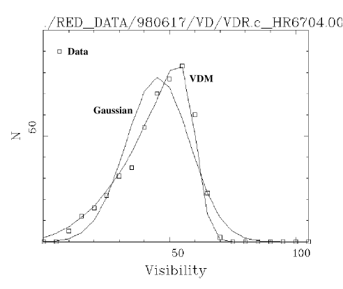
Figure 1: Comparison of visibility data in an observation (500 scans) with a Gaussian distribution and the visibility distribution model (VDM). In this case the visibility estimate given by the mean is $42.8\pm 0.6$%, while the estimate given by the VDM is $V=60.9\pm 0.3$%. The other VDM parameters obtained are: $\Delta\phi_{r}=0.15$ rad, $\sigma_{\Delta\phi_{r}}=0.15$ rad and $\sigma_{V_{noise}}=4$%.

2.2.3 Calibration

A spline interpolation between sequential $V$ estimates obtained in observations of calibrator sources, for which $V_{true}$ is known, yields a curve which reflects the time evolution of the instrument. Interleaved target observations, taken under identical instrumental conditions, are calibrated for the $V_{inst}$ term by dividing the target estimate by the interpolated calibrator estimate: $V_{true}^{target}=V_{true}^{cal}\cdot V^{target}/V^{cal}$. The spectral types and visual magnitudes of all the calibrator stars used in this paper (with the possible exception of HR8881, see section 3) have angular diameters less than $1-2$ mas, therefore, we use $V_{true}^{cal}=1.0$.

2.2.4 Errors

The internal uncertainty from fitting individual fringes is generally small ($\lesssim$1%), as is the formal uncertainty in the visibility for an observation obtained from the fit to the visibility distribution model ($\lesssim 2-3$%). However, the RMS of independent visibility measurements on the same object and at similar spatial frequencies is larger, typically $\lesssim$5% p-p (peak-to-peak) within a single night of observation, although larger, $\leq$15% p-p in H-band data and $\leq$20% p-p in K^′-band data, systematic differences occasionally exist when comparing data from different nights, both of which indicate the presence of low-frequency calibration errors. A likely explanation for this excess error is that our expectation that $r_{0}(H,K^{\prime})\sim D$ does not strictly hold, and that we see the effects of un-modelled wavefront curvature errors induced by the turbulent atmosphere. Therefore, the total uncertainty on an individual visibility measurement due to all sources is best represented by the RMS of independent measurements separated by hours of days. Using this measure, we find that the use of the visibility distribution model yields more consistent results, reducing the scatter of independent measurements by factors of $2-3$ compared to the mean estimator. This improvement is illustrated in Figure 2, which compares both methods on calibrated visibilities obtained on the same target on 4 nights of very different seeing conditions. We note that the night-to-night variations observed in this example are not believed to be due to the object itself (AB Aur) , but are instrumental. Variations in the object visibility are expected if (1) the source is asymmetric on the sky, or (2) it is composed of more than one component with changing relative fluxes. However, during one of the nights this source has been monitored for 5.2 hours (solid bullets in the plot), showing no sign of variation and implying a high degree of circular symmetry. Moreover, according to Voshchinnikov, Molster, & Thé (1996), AB Aur is an irregular photometric variable of very small amplitude, $\Delta m=\pm 0.02$. In a representation of the source consisting of a central star surrounded by near-IR emitting material such a small change in the brightness of the central star would result in a change of the observed visibility $<1$%, and therefore this effect is not likely to be the cause of the observed night-to-night variations.

Figure 2: Calibrated visibilities ($V_{true}$) obtained using the visibility distribution model (top panel) and the mean of the measured distribution (bottom panel). Each symbol represents data taken on the same source (AB Aur) on different nights covering a large range of seeing conditions, and using identical detection parameters. For reference, the longest set of data (filled bullets) spans 5.2 hours.

3 THE SAMPLE, LOG OF OBSERVATIONS, AND VISIBILITY AMPLITUDES

To date, the most complete and comprehensive compilation of candidate HAEBE stars is the catalog of 287 objects by Thé, de Winter, & Perez (1994). Our sample was selected from their Table 1, which contains 108 Ae and Be stars recognized as true members or good candidates of the HAEBE group, using as the selection criteria that the stars be brighter than the limiting magnitudes of IOTA’s tip-tilt servo system ($V=11-12$) and near-IR fringe detector (H=7, K^′=6.2). Furthermore, in order to have as homogenous a sample as possible, and in order to test the accretion disk hypothesis, we have primarily selected our sources to belong to Group I in the classification of HSVK. The only exceptions are $\omega$ Ori and MWC 166, which are Group III stars in that classification.

The final list of targets observed is presented in Table 3.2. Columns $1-3$ contain the star names and coordinates; columns $4-10$ show the VRIJHK photometry compilation, mostly from HSVK; columns $11-15$ contain stellar parameters, distance, visual extinction, spectral type and effective temperature, mostly from the Hipparcos data study of van den Ancker et al. (1998); and the last column comments on whether the star posseses a visual or spectroscopic companion and/or IR excess. Table 2 shows a log of the observations, including the calendar date, spectral band, calibrator used, the approximate hour angle (HA) range covered during the observation, a qualitative measure of the seeing at the time of the observations (1=very good, 4=bad) based on real-time visual inspection of the amount of atmospherically induced fringe piston and amplitude noise, and the baseline used (identified by its approximate length).

3.1 Special Cases and Visibility Correction Factors

3.1.1 Stars with Close Visual Companions

Using the technique of adaptive optics in the near-IR, Corporon (1998) surveyed 68 HAEBE stars and identified 30 binary systems with separations greater than 0.1 arcsec. We consider here the effect of those “wide” companions on our data set. Indeed, if a star has a companion at an angular offset such that it is in the detector’s field of view ($\sim 3\arcsec\times 3\arcsec$ for each pixel of the NICMOS3 camera), but whose interferogram has a zero OPD point that does not fall near that from the primary source, in the resulting scan a correction needs to be made to the fringe visibility measured on each interferogram that accounts for the incoherent flux added by the other star (exactly analogous to the incoherent flux added by thermal background, which needs to be subtracted before the fringe amplitude is measured). If we call $V_{true}^{j}$ the calibrated visibility corresponding to the bright ($j=A$) or faint ($j=B$) fringe obtained by the procedure described in Section 2.2, then the corrected visibility is given by

$$V_{true}^{{}^{\prime}j}=V_{true}^{j}/r_{j}\,;\quad\mbox{with:}\quad r_{A,B}=\frac{1}{(1+10^{\mp\Delta m/2.5})}$$ (4)

where $\Delta m=m_{B}-m_{A}$ is the magnitude difference between the binary components in the relevant spectral band.

Our sample overlaps almost perfectly with that of Corporon (1998), and therefore we use his measured binary separations and flux ratios to apply the above correction in the appropriate cases. Table 3.2 summarizes the angular separations ($\theta$), magnitude differences and the spectral types assigned to each component, for the subset of our sample for which the adaptive optics companion is approximately within the field of view of our NICMOS3 camera. Note that in our data set, the interferogram corresponding to the faint companion is never detected, either because it is too faint or because it occurs at a value of the OPD which is outside of the scan length. However, the correction by the $r_{A}$ factors, last two columns in Table 3.2, still needs to be applied to the fringe visibility corresponding to the bright component. The only two stars in our sample which were not observed by Corporon are AB Aur and V594 Cas, and we will assume here that they are single stars.

3.1.2 MWC 1080 and HR8881

The data for MWC 1080 shows that it is more resolved at H than at K^′, by an amount significantly greater than expected from the higher resolving power of the shorter H-band wavelength. In searching for explanations for this unusual circumstance, it was discovered that according to Hammersley et al. (1994), the calibrator used for MWC 1080 (HR 8881), is misclassified in the Bright Star Catalogue, and is really a M3 giant or K supergiant, and not a K1 dwarf.

Assuming that HR 8881 is a normal giant, we may estimate its angular size and account for it in the calibration of the MWC 1080 data. Based on a compilation of angular diameters measured in the near-IR by the techniques of lunar occultations and long baseline inteferometry, van Belle (1999) has derived empirical relations between angular diameters and $(V-K)$ and $(B-K)$ colors for main sequence, giants and supergiants stars. Using the photometry and $A_{V}=0.22$ estimate of Hammersley et al. (1994), we obtain $(V-K)=4.05\pm 0.02$ and $(B-K)=5.33\pm 0.02$. The empirical relations using those two colors predict uniform disk (UD) diameters $\theta=2.12\pm 0.28$ mas and $\theta=2.08\pm 0.37$ mas respectively. The weighted mean of the two predictions is $\theta=2.10\pm 0.22$ mas, which we adopt as our estimate of the angular size of HR 8881.

The visibility data for MWC 1080 has therefore been calibrated using the visibility that is expected for the estimated UD diameter $V_{cal}^{UD}=2\cdot J_{1}(\pi\theta s)/(\pi\theta s)$. For reference, for the baseline lengths corresponding to those obervations, this calibration factor is on average 0.95 for the H band observations and 0.97 for the K^′ band observations.

The unusual circumstance therefore remains that MWC 1080 is resolved by about 20% in H band observations and appears essentially unresolved in K^′ observations. This difference is difficult to explain with any simple model of the source, given that the near-IR excess is greater at K than at H, contributing 79% and 91% of the total flux at H and K respectively (see Section 4). One possible explanation would be that the calibrator, HR 8881, is not a UD, and that the interferometer resolves it at K^′ by a greater amount than is predicted by its photospheric extension. There are however no specific measurements in the literature to confirm or rule out this hypothesis, and a complete resolution to this question will have to await new observations at the IOTA of both MWC 1080 and HR 8881. If the result is confirmed, the apparent decrease in size with increasing wavelength could be explained if MWC 1080 is an under-resolved core-halo object. In this model, the small core contains the central star as well as the source of near-IR excess and dominates the emission at K^′ wavelengths, while at the shorter H wavelengths scattering reveals the larger angular extent of the cold halo component.

3.2 Visibility Data

The final set of calibrated H and K^′-band fringe visibility data is shown in Figure 3. The data are presented in two panels, one for each independent variable specifying the projection of the baseline vector in a plane ($u,v$) normal to the direction toward the source. The left panels show the data as a function of the modulus of the projected baseline: $s=\sqrt{u^{2}+v^{2}}$, expressed in millions of wavelengths at the center of the observation band. The left panels show the data as a function of the projected baseline position angle: $\Phi=\arctan\left(u/v\right)$, measured from North toward East. The size of the data symbols equals our typical uncertainty of 5% in the calibrated visibilities. In the case of the stars known to be adaptive optics binaries, only the bright component (A) detected interferometrically appears in the figure, and explicit error bars are shown reflecting the error in correction by the flux factor described in Section 3.1.1. The error bars in the data for MWC 1080 also include the contribution due to the uncertainty in the estimated size of HR 8881.

The detailed interpretation of this data set is the subject of the next two sections. However, based on inspection, we may immediately make the following observations: (1) of the 15 stars observed, 11 (73% of the sample) are resolved by the interferometer; (2) one star, MWC 361-A, shows the clear sinusoid signature of a binary system; (3) none of the other stars shows significant variation of visibility with baseline position angle (the range covered by the observations varies from $\Delta\Phi=0$ to $65\arcdeg$); and (4) of the two Group III sources, $\omega$ Ori appears unresolved, and MWC 166 appears only slightly resolved, both consistent with that classification.

Table 2: Log of Herbig Ae/Be Stars Observations

Date	Target	Band	Calibrator	HA	Seeing	Baseline
			(HR)			(m)
1997 Oct 13	AB Aur	H	1343,2219	$[-1.2,+0.6]$	2	21
1997 Nov 15	AB Aur	H	1626	$[-1.0,+3.0]$	1	38
1998 Jan 19	AB Aur	K′	1626	$[+0.9,+1.1]$	2	38
1998 Mar 02	AB Aur	K′	1626	$[+1.9,+2.1]$	1	21
1998 Mar 03	$\omega$ Ori	H	2019	$[+0.3,+0.7]$	2	21
		K′	2019	$[+0.9,+1.1]$	2	21
1998 Mar 07	AB Aur	H	1626	$[+1.6,+1.9]$	2	38
		K′	1626	$[+2.2,+2.5]$	2	38
1998 Jun 12	MWC 297	H	7149	$[+0.9,+1.2]$	3	38
	MWC 361	H	7967	$[-0.4,+0.2]$	3	38
1998 Jun 13	MWC 863	H	6153	$[-0.8,-0.5]$	2	38
	MWC 275	H	6704	$[-0.9,-0.1]$	2	38
	MWC 361	H	7967	$[+0.4,+0.7]$	1	38
1998 Jun 14	MWC 297	H	7149	$[-0.8,-0.0]$	2	38
1998 Jun 15	MWC 361	H	7967	$[-0.5,-0.0]$	1	38
1998 Jun 17	MWC 863	H	6153	$[-0.1,-0.5]$	1	38
	MWC 275	H	6704	$[-0.3,+1.4]$	1	38
	MWC 361	H	7967	$[-0.5,+0.7]$	1	38
1998 Jun 18	MWC 297	H	7066	$[-1.9,-1.6]$	1	38
	MWC 361	H	7967	$[-0.8,-0.2]$	1	38
		K′	7967	$[+0.0,+0.2]$	1	38
	MWC 1080	H	8881	$[-1.8,-1.4]$	1	38
1998 Jun 19	MWC 361	H	7967	$[-2.8,+1.0]$	1	38
		K′	7967	$[-2.1,+0.4]$	1	38
1998 Jun 20	MWC 361	H	7967	$[-4.9,+0.4]$	1	38
		K′	7967	$[-4.3,+0.6]$	1	38
	MWC 1080	H	8881	$[-3.5,-2.9]$	1	38
1998 Sep 28	MWC 361	H	7967	$[-0.7,+4.4]$	1	38
		K′	7967	$[+2.1,+3.7]$	1	38
1998 Sep 29	V1295 Aql	H	7669	$[+1.0,+2.4]$	2	38
1998 Sep 30	MWC 614	H	7449	$[+1.2,+2.4]$	1	38
1998 Oct 02	MWC 614	H	7449	$[+1.3,+2.2]$	1	38
	V1685 Cyg	H	7800	$[+2.4,+3.7]$	2	38
1998 Oct 31	MWC 1080	H	8881	$[+0.9,+2.9]$	1	38
		K′	8881	$[+1.8,+3.8]$	1	38
	T Ori	H	1986	$[-0.0,+0.4]$	1	38
1998 Nov 02	AB Aur	H	1626	$[-2.3,+2.9]$	1	38
1998 Nov 03	V594 Cas	H	237	$[-1.9,+0.8]$	1	38
	V380 Ori	H	1697	$[-1.8,-0.4]$	1	38
	MWC 147	H	2426	$[-0.2,+0.4]$	1	38
		K′	2426	$[+0.8,+1.3]$	1	38
1998 Nov 07	$\omega$ Ori	H	2019	$[-1.4,+2.0]$	3	38
1998 Nov 10	MWC 1080	K′	8881	$[+0.0,+3.0]$	2	38
	MWC 147	H	2426	$[-2.5,-0.0]$	2	38
	MWC 166	H	2723	$[+0.1,+1.5]$	3	38
1999 Mar 01	V380 Ori	H	1986	1.9	2	21
	MWC 863	H	6153	$[-0.8,-0.4]$	2	21
1999 Mar 02	MWC 863	H	2723	$[-2.3,-0.9]$	2	21
		K′	2723	”	2	21
1999 Mar 05	MWC 166	H	2723	$[+1.7,+2.2]$	2	38

Table 3: HAEBE stars with adaptive optics companions

Name	$\theta\arcsec$	$\Delta V$	$\Delta R$	$\Delta I$	$\Delta J$	$\Delta H$	$\Delta K$	SpTy	SpTy	$r_{A}(H)$	$r_{A}(K^{\prime})$
								A	B
V380 Ori	0.14	$\cdots$	0.10	$\cdots$	0.11	0.94	1.36	B7	G0	0.704 $\pm$ 0.040	0.778 $\pm$ 0.030
MWC 147	3.1	7.22	6.82	6.02	4.81	5.05	5.67	B2	K5	0.990 $\pm$ 0.002	0.995 $\pm$ 0.001
MWC 166	0.64	1.43	1.61	1.7	1.70	1.40	1.77	B0	B0	0.784 $\pm$ 0.030	0.836 $\pm$ 0.020
MWC 863	1.07	3.57	$\cdots$	2.57	2.07	2.24	2.72	A2	K4	0.887 $\pm$ 0.020	0.924 $\pm$ 0.010
V1685 Cyg	0.72	$\cdots$	$\cdots$	$\cdots$	$\cdots$	$\cdots$	5.50	B2	$\cdots$	$\cdots$	0.994 $\pm$ 0.001
MWC 361	2.55	5.40	5.04	4.52	$\cdots$	4.12	4.64	B2	G5	0.978 $\pm$ 0.004	0.986 $\pm$ 0.002
MWC 1080	0.77	2.34	2.44	2.61	$\cdots$	2.84	2.28	B2	B2	0.932 $\pm$ 0.010	0.891 $\pm$ 0.020

References. — Angular separation, photometric and spectral type data from Corporon (1998).

Note. — (1) Completeness limits: $0.1\arcsec\lesssim\theta\lesssim 7\arcsec$; $\Delta m<6-7$; (2) Uncertainties: $\sigma_{\theta}=0.05\arcsec$; $\sigma_{\Delta m}\lesssim 0.2$.

Figure 3: H and K^′-band calibrated visibility data. For each source, the data are plotted as a function of the projected baseline length ($s$, left panel) and position angle ($\Phi$, right panel). The different symbols correspond to observations on different nights, and retain their meaning between the right and left panels for a given source. Observations on the 21 m baseline are represented with filled symbols, and observations at the 38 m baseline with open symbols. All subsequent plots involving this visibility data retain the same symbols.

4 EXCESS NEAR-INFRARED FLUX

Most of the HAEBE stars in this paper are known to have a strong near-IR excess, and are resolved by the interferometer. Therefore, in order to interpret the visibility amplitude data we consider a two component model consisting of the central star, plus a component which is the source of the near-IR excess. However, before this model can be used to interpret the interferometer data, the relative contributions to the total H and K fluxes from these two components must be quantified. The notation used hereafter is as follows: “$T$”, “$\star$” and “$E$” superscripts denote total, stellar and excess fluxes respectively. Primed fluxes are apparent, while un-primed fluxes are intrinsic (i.e. corrected for extinction).

4.1 Stellar Flux

In order to estimate the stellar near-IR fluxes, we use the photometry data, visual stellar extinctions and stellar effective temperatures from the literature tabulated in Table 3.2. We assume that the short wavelength (VRI) flux arises entirely from the central star, and approximate the stellar spectrum as a blackbody at the adopted effective temperature. The solid angle subtended by the stellar disk of radius $R_{\star}$ at distance $d$, $\Omega_{\star}=\pi R_{\star}^{2}/d^{2}$, is the parameter adjusted in order to provide a best fit to the de-reddened V, R and I fluxes, according to: $F_{VRI}^{\star}=B_{VRI}(T_{eff})\cdot\Omega_{\star}$, where $B_{\nu}(T)$ denotes the Planck function. The literature flux data has been de-reddened using the extinction law ($A_{\lambda}/A_{V}$) of Steenman & Thé (1991) and a ratio of total to selective extinction $R=A_{V}/E_{B-V}=3.10$. Once the solid angle factor is thus determined, the stellar flux may be calculated at any frequency as $F_{\nu}^{\star}=B_{\nu}(T_{eff})\cdot\Omega_{\star}$, and used to quantify the flux in excess of the photospheric value.

The literature flux data is quoted as having uncertainties of 0.01$-$0.02 mag in the VRI bands. In addition, the spectral classification is uncertain by 1 sub-class typically, which results in about 0.2 mag uncertainty in the derived values of the visual extinction and about 11% uncertainty in the effective temperatures. The resulting relative uncertainties in the predicted near-IR stellar fluxes are in the range $17\%-50\%$ (median 30%).

In the case of those sources which were identified as adaptive optics binaries by Corporon, we calculate the SED of each component by combining the magnitude differences of Table 3.2 with the total photometry of Table 3.2. We determine effective temperatures for each component using the spectral types assigned by Corporon and the temperature scale of Cohen & Kuhi (1979). These effective temperatures are used to calculate the blackbody model which represents the photospheric contribution of each star to the total flux, as described above for the single stars.

4.2 Excess Flux

Using this model to represent the stellar photosphere, we may deduce the apparent excess fluxes due to CS emission: $F^{\prime E}_{JHK}=F^{\prime T}_{JHK}-F^{\star}_{JHK}\cdot 10^{-A^{\star}_{JHK}/2.5}$, where the apparent total fluxes and visual stellar extinctions are the observed quantities from the literature. Estimating the intrinsic (i.e. de-reddened) excess fluxes is also of interest, since they directly relate to the physical properties of the source. This however, requires knowledge of the amount of attenuation suffered by the excess radiation between the source and the observer, while the only information available is the total extinction in the line of sight toward the star. Therefore, we adopt here the simplifying assumptions that (1) all of the stellar extinction is due to cold foreground material, and (2) it is the same for all lines of sight that intercept the extended component, so that $F^{E}_{JHK}=10^{+A^{\star}_{JHK}/2.5}\cdot F^{\prime E}_{JHK}$.

Figure 4 shows the de-reddened SED data and best fit stellar blackbody models for all the target stars. Note that in most cases the individual components in the adaptive optics binaries also have significant IR excess.

The results for the derived H and K stellar fluxes are summarized in Table 4. In addition to the quantities already defined, the fourth column lists the stellar angular diameters that are implied by the solid angle calculated, $\theta^{\star}=2\sqrt{\Omega/\pi}$, and it can be seen that the values obtained are all small compared to the resolution of the interferometer. Therefore, in our models of the brightness distribution, the central stars will be treated as point sources.

Table 5 summarizes the results obtained for the excess fluxes. The errors are dominated by the uncertainty in the determination on the underlying stellar spectrum, as described in the previous section, and include an uncertainty of $0.01-0.1$ mag from the total near-IR magnitudes in the literature, as well as a small contribution due to the uncertainty in the extinction at near-IR wavelengths derived from the visual extinctions. The last column in Table 5 contains the color temperature ($T_{c}$) of the excess emission, calculated from the intrinsic H and K excesses such that $F^{E}_{H}/F^{E}_{K}=B_{H}(T_{c})/B_{K}(T_{c})$.

Figure 4: Total SED data and photospheric models. Each panel shows the de-reddened total SED data of a target (circles) and the stellar blackbody model (dashed lines) corresponding to the underlying star. In the case of the adaptive optics binaries (Corporon 1998), the SED data for each component is also shown (open squares and triangles) and the solid line represents the sum of the two model photospheres.

Table 4: Near-IR stellar fluxes

Name	$\mbox{log}(T_{\mbox{eff}})$	$\Omega_{\star}$	$\theta_{\star}$	$F^{\star}_{H}$	$F^{\star}_{K}$	$A_{H}$	$A_{K}$	$F^{\prime\star}_{H}$	$F^{\prime\star}_{K}$
		($10^{-20}$ sr)	(mas)	(Jy)	(Jy)			(Jy)	(Jy)
V594 Cas	4.08	06.3	0.06	0.5 $\pm$ 0.1	0.3 $\pm$ 0.1	0.3	0.2	0.4 $\pm$ 0.1	0.3 $\pm$ 0.1
AB Aur	3.98	50.3	0.2 0	3.0 $\pm$ 1.1	1.9 $\pm$ 0.7	0.07	0.04	2.8 $\pm$ 1.0	1.8 $\pm$ 0.7
T Ori	4.03	05.4	0.05	0.4 $\pm$ 0.1	0.2 $\pm$ 0.1	0.2	0.1	0.3 $\pm$ 0.1	0.2 $\pm$ 0.1
V380 Ori-A	4.09	02.2	0.03	0.2 $\pm$ 0.05	0.1 $\pm$ 0.03	0.2	0.1	0.1 $\pm$ 0.04	0.1 $\pm$ 0.03
$\omega$ Ori	4.23	98.0	0.2 0	12.9 $\pm$ 3.8	7.8 $\pm$ 2.4	0.04	0.02	12.4 $\pm$ 3.7	7.6 $\pm$ 2.3
MWC 147-A	4.31	06.0	0.06	1.0 $\pm$ 0.2	0.6 $\pm$ 0.1	0.2	0.1	0.8 $\pm$ 0.2	0.5 $\pm$ 0.1
MWC 166-A	4.49	22.0	0.05	6.0 $\pm$ 1.3	3.5 $\pm$ 0.8	0.3	0.2	4.2 $\pm$ 0.9	2.9 $\pm$ 0.6
MWC 863-A	3.96	30.9	0.1 0	1.7 $\pm$ 0.6	1.1 $\pm$ 0.4	0.2	0.1	1.3 $\pm$ 0.5	1.0 $\pm$ 0.3
MWC 275	3.97	51.2	0.2 0	2.9 $\pm$ 1.1	1.9 $\pm$ 0.8	0.03	0.02	2.8 $\pm$ 1.1	1.8 $\pm$ 0.7
MWC 297	4.53	60.7	0.2 0	18.3 $\pm$ 3.4	10.6 $\pm$ 2.0	1.2	0.7	6.3 $\pm$ 1.2	5.8 $\pm$ 1.1
MWC 614	4.02	19.6	0.1 0	1.3 $\pm$ 0.4	0.8 $\pm$ 0.3	0.2	0.1	1.1 $\pm$ 0.4	0.8 $\pm$ 0.2
V1295 Aql	3.95	24.9	0.1 0	1.3 $\pm$ 0.5	0.9 $\pm$ 0.3	0.03	0.01	1.3 $\pm$ 0.4	0.8 $\pm$ 0.3
V1685 Cyg	4.34	04.1	0.05 0	0.7 $\pm$ 0.2	0.4 $\pm$ 0.1	0.4	0.2	0.5 $\pm$ 0.1	0.4 $\pm$ 0.1
MWC 361-A	4.31	29.5	0.1 0	4.9 $\pm$ 1.2	2.9 $\pm$ 0.7	0.3	0.1	3.6 $\pm$ 0.9	2.5 $\pm$ 0.6
MWC 1080-A	4.31	10.4	0.07 0	1.7 $\pm$ 0.4	1.0 $\pm$ 0.2	0.7	0.4	0.8 $\pm$ 0.2	0.7 $\pm$ 0.2

Table 5: Near-IR excess fluxes

Name	$F^{\prime T}_{H}$	$F^{\prime T}_{K}$	$F^{\prime E}_{H}$	$F^{\prime E}_{K}$	$(F^{\prime E}/F^{\prime T})_{H}$	$(F^{\prime E}/F^{\prime T})_{K}$	$F^{E}_{H}$	$F^{E}_{K}$	$T_{c}$
	(Jy)	(Jy)	(Jy)	(Jy)	(%)	(%)	(Jy)	(Jy)	(K)
V594 Cas	1.7 $\pm$ 0.1	3.3 $\pm$ 0.2	1.3 $\pm$ 0.1	3.0 $\pm$ 0.2	76.2 $\pm$ 7.0	91.5 $\pm$ 2.7	1.7 $\pm$ 0.2	3.5 $\pm$ 0.2	1382 $\pm$ 117
AB Aur	8.9 $\pm$ 0.4	10.8 $\pm$ 0.5	6.1 $\pm$ 1.1	8.9 $\pm$ 0.9	68.7 $\pm$ 11.5	82.9 $\pm$ 6.5	6.5 $\pm$ 1.2	9.3 $\pm$ 0.9	1814 $\pm$ 331
T Ori	1.2 $\pm$ 0.01	2.0 $\pm$ 0.1	0.9 $\pm$ 0.1	1.8 $\pm$ 0.1	74.8 $\pm$ 8.6	89.5 $\pm$ 3.7	1.1 $\pm$ 0.1	2.0 $\pm$ 0.1	1503 $\pm$ 110
V380 Ori-A	0.9 $\pm$ 0.05	1.8 $\pm$ 0.1	0.8 $\pm$ 0.1	1.7 $\pm$ 0.1	84.3 $\pm$ 4.3	94.2 $\pm$ 1.6	1.0 $\pm$ 0.1	1.9 $\pm$ 0.1	1457 $\pm$ 113
$\omega$ Ori	12.6 $\pm$ 0.6	8.1 $\pm$ 0.4	0.1 $\pm$ 3.7	0.5 $\pm$ 2.4	0.9 $\pm$ 29.8	5.9 $\pm$ 29.1	0.1 $\pm$ 3.8	0.5 $\pm$ 2.4	$\cdots$
MWC 147-A	2.1 $\pm$ 0.1	3.3 $\pm$ 0.2	1.3 $\pm$ 0.2	2.8 $\pm$ 0.2	62.8 $\pm$ 9.2	84.3 $\pm$ 3.9	1.7 $\pm$ 0.3	3.2 $\pm$ 0.2	1467 $\pm$ 189
MWC 166-A	4.7 $\pm$ 0.2	4.2 $\pm$ 0.2	0.5 $\pm$ 0.9	1.3 $\pm$ 0.7	11.7 $\pm$ 20.1	31.2 $\pm$ 15.8	0.8 $\pm$ 1.4	1.6 $\pm$ 0.8	1408 $\pm$ 1690
MWC 863-A	2.6 $\pm$ 0.1	3.6 $\pm$ 0.2	1.2 $\pm$ 0.5	2.6 $\pm$ 0.4	47.8 $\pm$ 18.2	73.1 $\pm$ 9.8	1.6 $\pm$ 0.6	3.0 $\pm$ 0.4	1471 $\pm$ 405
MWC 275	5.8 $\pm$ 0.3	8.0 $\pm$ 0.4	3.0 $\pm$ 1.1	6.2 $\pm$ 0.8	51.1 $\pm$ 19.0	77.0 $\pm$ 9.3	3.1 $\pm$ 1.2	6.3 $\pm$ 0.9	1393 $\pm$ 375
MWC 297	14.4 $\pm$ 0.7	36.3 $\pm$ 1.8	8.2 $\pm$ 1.4	30.6 $\pm$ 2.1	56.6 $\pm$ 8.5	84.1 $\pm$ 3.1	23.8 $\pm$ 4.2	56.3 $\pm$ 4.1	1268 $\pm$ 143
MWC 614	2.0 $\pm$ 0.1	2.7 $\pm$ 0.1	0.9 $\pm$ 0.4	1.9 $\pm$ 0.3	44.7 $\pm$ 17.8	71.4 $\pm$ 9.6	1.1 $\pm$ 0.4	2.1 $\pm$ 0.3	1453 $\pm$ 387
V1295 Aql	2.3 $\pm$ 0.1	3.0 $\pm$ 0.1	1.0 $\pm$ 0.5	2.2 $\pm$ 0.3	44.0 $\pm$ 19.8	72.0 $\pm$ 10.3	1.0 $\pm$ 0.5	2.2 $\pm$ 0.3	1325 $\pm$ 424
V1685 Cyg	1.7 $\pm$ 0.1	3.0 $\pm$ 0.1	1.2 $\pm$ 0.1	2.7 $\pm$ 0.2	70.6 $\pm$ 7.2	88.4 $\pm$ 2.9	1.8 $\pm$ 0.2	3.4 $\pm$ 0.2	1463 $\pm$ 126
MWC 361-A	6.0 $\pm$ 0.3	8.1 $\pm$ 0.4	2.4 $\pm$ 0.9	5.6 $\pm$ 0.7	40.5 $\pm$ 14.8	69.4 $\pm$ 7.7	3.3 $\pm$ 1.3	6.6 $\pm$ 0.9	1408 $\pm$ 387
MWC 1080-A	3.6 $\pm$ 0.2	7.3 $\pm$ 0.4	2.9 $\pm$ 0.3	6.6 $\pm$ 0.4	79.2 $\pm$ 5.2	91.0 $\pm$ 2.3	6.6 $\pm$ 0.6	10.4 $\pm$ 0.7	1673 $\pm$ 151

5 MODELS OF THE BRIGHTNESS DISTRIBUTION

The small sizes of the central stars derived in Section 4 imply that the interferometer resolves the CS material source of the excess emission. In this section we make use of the interferometer data to characterize the geometrical distribution of this CS material. This information, together with the intrinsic excess fluxes derived in Section 4, permits the brightness distribution to be estimated.

5.1 A Source with no IR Excess: $\omega$ Ori

The visibility data of Figure 5 shows that $\omega$ Ori is unresolved by the interferometer. Moreover, it was shown in Section 4 that there is no significant IR excess associated with this star. Consequently, we will place a size limit to the star itself by considering a single uniform disk (UD) component.

Using the visibility data obtained at the longest 38 m baseline, which provides the highest angular resolution, the mean fringe spacing projected on the sky is $s=21.1M\lambda$ and the mean visibility is $V=100.5\pm 2.0\%$, where the error is the error in the mean of the 5 long baseline measurements. Therefore the minimum visibility allowed by the data is $V_{min}=96.5\%$ and by solving in the equation for the UD visibility (recall Section 3.1.2) it is found that the upper limit to the UD angular diameter is $\theta\leq 1.3$ mas, at the $2\sigma$ level. The data and visibility function corresponding to this upper limit are shown in Figure 5.

We note that among our sample, this is the source which most clearly shows the absence of IR excess above photospheric levels (see Figure 4), and as such was classified as Group III by HSVK. Therefore, observations of this source are valuable as a control experiment, and our result is indeed consistent with it being a naked photosphere.

Figure 5: $\omega$ Ori visibility data (H-band) and model curve corresponding to the upper limit UD diameter ($\theta\leq 1.3$ mas).

5.2 Models of the Source of IR Excess

For the remainder of our sample, we consider four plausible models of the source brightness. Each model has two components, with the stellar emission arising in a central point source and the excess near-IR emission contributed by either: (1) a Gaussian brightness distribution, (2) a uniformly bright ring, (3) an infrared companion or (4) a “classical” accretion disk with a temperature law $T(r)\propto r^{-3/4}$. The Gaussian and ring models are intended to provide a characteristic size for the source of near-IR excess, and consistent with the observation that the visibilities remain constant with projected baseline orientation, we consider the simplest case that they appear circularly symmetric on the sky.

In general, the source specific intensity (i.e. brightness) is given by

$$I_{\nu}(\xi,\eta)=F^{\star}_{\nu}\cdot\delta(0,0)+I^{E}_{\nu}(\xi,\eta)\\$$ (5)

and the corresponding normalized visibility amplitude is calculated by application of the Van Cittert-Zernike theorem (see e.g. Goodman 1985)

$$V_{\nu}(u,v)=\left|\frac{\mbox{FT}\{I_{\nu}(\xi,\eta)\}}{F^{\star}_{\nu}+F^{E}_{\nu}}\right|=\left|\frac{F^{\star}_{\nu}+\mbox{FT}\{I^{E}_{\nu}(\xi,\eta)\}}{F^{\star}_{\nu}+F^{E}_{\nu}}\right|$$ (6)

where in the above equations, $(\xi,\eta)$ are angular offsets with respect to the source center along the projected baseline coordinates $(u,v)$ measured in wavelength units (see e.g. Thompson, Moran, & Swenson 1986), and FT denotes the Fourier transform.

In addition to $\omega$ Ori, we find 3 more sources which appear unresolved, namely V594 Cas, T Ori and MWC 147. However, since in those cases there is significant near-IR excess (see Figure 4), we will place appropriate upper limits to the extended component within the context of the models considered. The source MWC 166 appears to have low visibility ($V=88.2\pm 0.9$ %). However, it was found in the previous chapter to have a marginally significant amount of near-IR excess flux, with $88\pm 20$ % of the total H flux arising in the central star. The data is therefore consistent with this source having an extended component which is completely resolved by the interferometer. Given the large error in the derived excess flux however, we cannot rule out the possibility that there is zero excess, so that all the emission comes from the star alone, or that the interferometer only partially resolves an extended component which contributes a larger fraction (up to 32%) of the total H flux. In this case then, lower limits will be given for the size of the excess region under the models mentioned above.

5.2.1 Gaussian Intensity

We consider a circularly symmetric brightness distribution given by

$$I^{E}_{\nu}(\xi,\eta) = I^{0}_{\nu}\cdot e^{\frac{-4\ln 2(\xi^{2}+\eta^{2})}{\theta_{G}^{2}}}$$ (7)

so that

$$V_{\nu}(s) = \left|\frac{F^{\star}_{\nu}+F^{E}_{\nu}\cdot e^{\frac{-\pi^{2}s^{2}\theta_{G}^{2}}{4\ln 2}}}{F^{\star}_{\nu}+F^{E}_{\nu}}\right|$$ (8)

where $I^{0}_{\nu}$ is the peak intensity and $\theta_{G}$ is the angular FWHM in both sky coordinates ($\xi$ and $\eta$).

Once the Gaussian FWHM is found by fitting Equation 8 to the visibility data, the peak intensity is obtained from the constraint that the flux in this component matches the measured excess flux

$$F^{E}_{\nu}=\int\int I^{0}_{\nu}\cdot e^{\frac{-4\ln 2(\xi^{2}+\eta^{2})}{\theta_{G}^{2}}}d\xi d\eta=I^{0}_{\nu}\cdot\Omega_{G}$$

where $\Omega_{G}=\pi^{2}\theta_{G}^{2}/4\ln 2$, is the effective solid angle. In practice, we find it most informative to express the peak intensity in terms of the equivalent peak brightness temperature, defined by $I^{0}_{\nu}=B_{\nu}(T^{0}_{B})$. The brightness temperature can then be readily compared with the color temperature derived from the H and K excess fluxes in order to determine whether this model is consistent with blackbody emission at the color temperature of the H and K excess.

Table 6 summarizes the results obtained. In addition to the best fitting Gaussian FWHM, the table includes the RMS of the fit evaluated as $\sqrt{\chi^{2}_{min}/(N-1)}$ with $\chi^{2}=\sum_{i=1}^{N}(V^{data}_{i}-V^{model}_{i})^{2}$, the number of individual observations for each star (N), the linear diameter (D) corresponding to the measured angular diameter calculated using the distances of Table 3.2, and the peak brightness temperature ($T^{0}_{B}$) calculated as described above. For the two stars which were observed in both the H and K^′ bands and are resolved (AB Aur and MWC 863-A), it is found that the sizes in this model are, within the errors, the same, and the table shows in those cases the size that is derived from a simultaneous fit to both data sets. For the other stars, for which an independent measurement of the size in the K^′-band is not available, the peak brightness temperature at K^′ is calculated using the size derived from fitting the H-band data. In all cases (as well as in the following tables corresponding the other models under consideration), the errors in the angular sizes reflect the uncertainty in the relative flux in each component, given in Table 5, rather than the much smaller formal error (of order 0.1 mas) associated with fitting a given set of visibility data. Figure 6 shows the data and models (solid lines) computed with the parameters of Table 6.

We note that for AB Aur, a slightly better agreement is obtained by fitting the H and K^′-band data sets separately. In that case we derive: $\theta_{G}^{H}\,=\,4.1\pm 0.5$ mas and $\theta_{G}^{K^{\prime}}\,=\,4.6\pm 0.2$ mas, with fit RMS of 3.4% and 5.9% respectively, to be compared to 3.5% and 9.6% obtained by fitting the model of Table 6 to the H and K^′ data separately. However, although formally a better fit, the different H and K^′-band sizes are within their errors. In Millan-Gabet et al. (1999b), based on a smaller data set and using a different data reduction method, the opposite result was obtained, that the characteristic size for AB Aur appeared somewhat smaller in the K^′ band than in the H band; although the difference was again judged to be most likely insignificant. This important question will need to be settled through improved accuracy of our visibility calibration.

Table 6: Gaussian model parameters.

Name	$\theta_{G}$	Fit RMS	N	D	H-band $T^{0}_{B}$	K′-band $T^{0}_{B}$
	(mas)	(%)		(AU)	(K)	(K)
V594 Cas	$\leq$ 0.8	$\cdots$	6	$\leq$ 0.5	$\geq$ 1938	$\geq$ $2212$
AB Aur	4.1 $\pm$ 0.5	4.6	47	0.6 $\pm$ 0.1	1359 $\pm$ 65 0	1258 $\pm$ 63 0
T Ori	$\leq$ 1.4	$\cdots$	2	$\leq$ 0.6	$\geq$ 1443	$\geq$ $1424$
V380 Ori-A	2.4 $\pm$ 0.1	2.0	8	1.1 $\pm$ 0.05	1208 $\pm$ 22 0	1144 $\pm$ $20$ 0
MWC 147-A	$\leq$ 1.0	$\cdots$	9	$\leq$ 0.8	$\geq$ 1765	$\geq$ 1884
MWC 166-A	$\geq$ 4.5	$\cdots$	8	$\geq$ 5.2	$\leq$ 1003	$\leq$ $916$
MWC 863-A	7.6 $\pm$ 1.7	6.7	18	1.1 $\pm$ 0.3	0963 $\pm$ 44 0	0865 $\pm$ 21 0
MWC 275	$4.6^{+1.7}_{-0.8}$	2.8	9	$0.6^{+0.2}_{-0.1}$	1175 $\pm$ 104	1124 $\pm$ 104
MWC 297	$5.8^{+0.9}_{-0.5}$	2.0	10	$2.6^{+0.4}_{-0.2}$	1500 $\pm$ 77 0	1594 $\pm$ $92$ 0
MWC 614	$7.6_{-2.5}$	2.0	13	$1.8_{-0.6}$	0923 $\pm$ 74 0	0826 $\pm$ $70$ 0
V1295 Aql	$5.4_{-1.4}$	4.3	4	$\cdots$	0991 $\pm$ 78 0	0910 $\pm$ $68$ 0
V1685 Cyg	2.6 $\pm$ 0.1	2.8	3	2.5 $\pm$ 0.1	1284 $\pm$ 30 0	1235 $\pm$ $30$ 0
MWC 1080-A	2.7 $\pm$ 0.2	6.4	20	5.9 $\pm$ 0.2	1566 $\pm$ 33 0	1535 $\pm$ 35 0

By comparing the peak brightness temperatures of Table 6 with the color temperatures of Table 5, it is apparent that for most objects, the brightness temperature is lower than the color temperature. One possible physical scenario for the Gaussian model is as an approximation to the brightness resulting from a circumstellar environment in which the dust particles are distributed in an envelope around the central star. A possible interpretation then is that the near-IR emission is optically thin, in which case the observed color temperature depends on the physical temperature of the dust grains, their emission properties and the optical depth of the CS cloud. We now further explore the consequences of this observation under the simplifiying assumption that a single temperature characterizes the dust envelope. If the near-IR frequency dependence of the optical depth in the circumstellar environment of HAEBE stars follows the properties characteristic of interstellar dust ($A_{V}\sim\lambda^{-1.9}$, due to dust particles smaller than the wavelength of light), we may derive the physical temperature (T) of the grains and the peak optical depth by solving in

$$\mbox{\bf Case A:\hskip 7.22743pt}\left\{\begin{array}[]{lll}B_{H}(T^{0}_{B})&=&B_{H}(T)\cdot(1-e^{-\tau^{0}_{H}})\\ B_{K}(T^{0}_{B})&=&B_{K}(T)\cdot(1-e^{-\tau^{0}_{K}})\\ \tau^{0}_{H}/\tau^{0}_{K}&=&A_{H}/A_{K}=1.75\end{array}\right.$$ (9)

where the ratio of H to K-band extinction has again been taken from Steenman & Thé (1991) with $R_{V}=3.1$.

On the other hand, from studies of the stellar extinction toward HAEBE stars, some authors find evidence for anomalous extinction laws ($R_{V}\simeq 5$) indicative of the presence of a significant population of grains with sizes greater (radius $a\sim 0.2\,\mu$m) than the average in the interstellar medium (Djie & Thé, 1978; Pezzuto, Strafella, & Lorenzetti, 1997). In the limit that the dust grains become larger than the wavelength of light, the cross-section for absorption and scattering becomes independent of wavelength and results in neutral extinction (as in interplanetary dust grains, of $a\sim 1-100\,\mu m$). Therefore, we also compute the peak optical depth that results from making the assumption that the opacity is wavelength independent

$$\mbox{\bf Case B:\hskip 7.22743pt}B_{\nu}(T^{0}_{B})=B_{\nu}(T_{C})\cdot\left(1-e^{-\tau^{0}}\right)$$ (10)

The results obtained under these two assumptions are summarized in Table 7. The “Case A” assumption results in an estimate of the physical temperature (T) of the dust grains and H-band peak optical depth, as well as the visual extinction of the star due to the CS cloud that would be implied, calculated according to $A_{V}=A_{H}/0.14=(\tau_{H}/2)\cdot(2.5/0.14\ln 10)$. For the “Case B” assumption, the physical temperature equals the color temperature of Table 5, and we calculate the frequency independent peak optical depth ($\tau^{0}$) and the corresponding visual extinction, $A_{V}=(\tau/2)\cdot(2.5/\ln 10)$. Finally, for comparison, the table reproduces in the last column the measured value of the visual extinction toward the star obtained from the literature (see Table 3.2).

Table 7: Gaussian model temperature and peak optical depth.

	Case A			Case B		Measured
Name	T	$\tau_{H}^{0}$	$A_{V}$	$\tau^{0}$	$A_{V}$	$A_{V}$
	(K)			($T=T_{C}$)
AB Aur	1423 $\pm$ 61	1.4 $\pm$ 0.1	5.3	00.2 $\pm$ 0.1 0	0.1	0.5
V380 Ori-A	1238 $\pm$ 23	1.8 $\pm$ 0.1	5.8	00.3 $\pm$ 0.05	0.2	1.43
MWC 863-A	1104 $\pm$ 110	0.4 $\pm$ 0.2	1.5	0.04 $\pm$ 0.02	0.02	1.61
MWC 275	1195 $\pm$ 100	2.1 $\pm$ 0.3	8.2	00.4 $\pm$ 0.2 0	0.2	0.25
MWC 297	$\cdots$	$\cdots$	$\cdots$	$\cdots$	$\cdots$	8.3
MWC 614	1074 $\pm$ 58	0.3 $\pm$ 0.1	1.2	0.03 $\pm$ 0.01	0.02	1.27
V1295 Aql	1072 $\pm$ 86	0.7 $\pm$ 0.1	2.7	00.1 $\pm$ 0.05	0.06	0.19
V1685 Cyg	1299 $\pm$ 30	2.5 $\pm$ 0.1	9.7	00.6 $\pm$ 0.1 0	0.3	3.16
MWC 1080-A	1570 $\pm$ 65	4.1 $\pm$ 0.1	15.9	01.2 $\pm$ 0.1 0	0.6	5.27

Note. — The optical depths and temperatures in this table are rounded from the solutions to equations 10 and 11, the resulting numerical loss of accuracy is however within the qouted error bars, which result primarily from the uncertainties in the excess fluxes.

From the results in the last two tables, we extract the following conclusions. First, the observed fluxes and our measured sizes are consistent with emission from dust envelopes having finite optical thickness (i.e. $T^{0}_{B}<T_{C}$), in 10 out of 13 cases, even at the position of the peak intensity. We note that under the other extreme assumption concerning the extinction of excess emission, i.e. that it is zero and this material causes all of the stellar extinction, the intrinsic excess fluxes would be given by columns 4 and 5 of Table 5, which are lower and would lead to even smaller values of the peak brightness and peak optical depths inferred. The unphysical result $T^{0}_{B}>T_{C}$ is found for one of the resolved sources (MWC 297) and for two of the three unresolved sources (V594 Cas and MWC 147), inconsistently with the model assumptions, and is most likely a consequence of the inadequacy of the assumption that there is a single temperature throughout the envelope rather than a radial temperature gradient. Second, the assumption that the extinction properties in the envelope are interstellar (case A) leads to relatively large values of the visual extinction (median $A_{V}=5.8$) in the line of sight toward the central stars. Under this assumption then, a special geometry that allows a clear line of sight to the star itself would need to be invoked, as has been proposed by Berrilli et al. (1992) and Hartmann, Kenyon, & Calvet (1993) in the context of SED modelling. Third, under the assumption that the extinction in the envelope is neutral (case B), the visual extinctions to the stars (median $A_{V}=0.2$) are somewhat lower than the measured values. However, the values derived are lower limits, and therefore consistent with the observed ones, since they do not include an interstellar contribution, or a contribution from the larger particles that are likely to exist in a realistic distribution of sizes.

5.2.2 Uniform Ring

In the previous section it was shown that under the Gaussian model, the effective sizes measured by the interferometer require that the emission be optically thin over most of the area of the source, in order to match the observed fluxes. An alternative solution is to consider optically thick emission at the observed color temperature, but reduce the emitting surface area by concentrating it in a narrow ring around the star.

For a uniform ring of intensity $I_{\nu}=B_{\nu}(T_{C})$, and inner and outer angular diameters $\theta_{1}$ and $\theta_{2}$ respectively, we have

$$I^{E}_{\nu}(\xi,\eta) = \left\{\begin{array}[]{ll}B_{\nu}(T_{C})&\mbox{if $\quad\frac{1}{2}\theta_{1}\leq\sqrt{\xi^{2}+\eta^{2}}\leq\frac{1}{2}\theta_{2}$}\\ 0&\mbox{otherwise}\end{array}\right.$$ (13)

$$V_{\nu}(s) = \left|\frac{F^{\star}_{\nu}}{F^{T}_{\nu}}+\frac{F^{E}_{\nu}}{F^{T}_{\nu}}\cdot\frac{4}{\pi\left(\theta_{2}^{2}-\theta_{1}^{2}\right)}\cdot\left[\frac{\theta_{2}\cdot J_{1}(\pi\theta_{2}s)}{2s}-\frac{\theta_{1}\cdot J_{1}(\pi\theta_{1}s)}{2s}\right]\right|$$ (14)

where for each value of the inner diameter, the outer diameter is constrained by the requirement that the flux from the ring matches the excess flux: $\theta_{2}=\sqrt{4\Omega/\pi+\theta_{1}^{2}}$ with $\Omega=F^{E}_{\nu}/B_{\nu}(T_{C})$. The only parameter to be fit to the visibility data is then the ring inner diameter.

The results are shown in Table 8, where in addition to the quantities already defined, the last two columns contain the linear ring inner and outer diameters. Figure 6 shows the data and models (dot-short dash lines) computed with the parameters of Table 8. We note that the source V594 Cas (which appears unresolved) can not be represented by this model, due to the fact that for any inner ring diameter, the outer diameter required to match the excess flux results in a source that would appear resolved. Similarly, the large excess flux for MWC 297 implies that any solution for the ring model has a large size, much larger than the characteristic size given by the Gaussian model. The data can formally be well fit only at the peak of the second lobe of the ring visibility function, and we do not consider this a likely interpretation of the data for this source.

Table 8: Ring model parameters.

Name	$\theta_{1}$	FitRMS	N	$\theta_{2}$	$D_{1}$	$D_{2}$
	(mas)	(%)		(mas)	(AU)	(AU)
V594 Cas	$\cdots$	$\cdots$	$\cdots$	$\cdots$	$\cdots$	$\cdots$
AB Aur	4.2 $\pm$ 0.40	5.2	47	4.7 $\pm$ 0.40	0.60$\pm$ 0.05	0.7 $\pm$ 0.05
T Ori	$\leq$ 1.40	$\cdots$	2	$\leq$ 2.05	$\leq$ 0.6	$\leq$ 0.9
V380 Ori-A	2.5 $\pm$ 0.10	2.0	8	3.0 $\pm$ 0.10	1.15 $\pm$ 0.50	1.4 $\pm$ 0.05
MWC 147-A	$\leq$ 0.4	$\cdots$	12	$\leq$ 2.0	$\leq$ 0.3	$\leq$ 1.6
MWC 166-A	$\geq 9.5$	2.5	8	$\geq 9.6$	$\geq 10.9$	$\geq 11.0$
MWC 863-A	$8.2^{+2.7}_{-1.5}$	6.2	18	$8.5^{+2.7}_{-1.5}$	$1.2^{+0.4}_{-0.2}$	$1.3^{+0.4}_{-0.2}$
MWC 275	$4.7^{+1.7}_{-0.9}$	3.1	9	$5.7^{+1.4}_{-0.8}$	$0.6^{+0.2}_{-0.1}$	$0.7^{+0.2}_{-0.1}$
MWC 297	$21.9^{+1.2}$	4.1	10	$25.0^{+1.0}$	$9.9^{+0.5}$	$11.25^{+0.45}$
MWC 614	6.7 $\pm$ 1.50	2.3	13	6.9 $\pm$ 1.40	1.60$\pm$ 0.40	1.7 $\pm$ 0.30
V1295 Aql	$5.4_{-1.2}$	4.4	4	$5.8_{-1.1}$	$\cdots$	$\cdots$
V1685 Cyg	2.7 $\pm$ 0.15	2.8	3	3.4 $\pm$ 0.15	2.55 $\pm$ 0.15	3.3 $\pm$ 0.15
MWC 1080-A	2.3 $\pm$ 0.30	9.0	20	3.6 $\pm$ 0.30	5.10$\pm$ 0.70	7.9 $\pm$ 0.70

Figure 6: Visibility data and Gaussian and ring models. Solid lines: Point source plus Gaussian intensity model. Dot-short dashed lines: Point source plus uniform ring model. The models are calculated for the best fit parameters of Tables 6 and 8.

5.2.3 Accretion Disk

Given that the stars in our sample which the interferometer resolves are all Group I sources in the classification of HSVK, we consider in this section whether such an accretion disk model is consistent with the interferometer data.

We consider a flat, blackbody disk heated by a central star of effective temperature $T_{\mbox{eff}}$ and radius $R_{\star}$. Energy balance between stellar light absorbed at distance $r$ by one side of the disk and subsequent re-radiation at the equilibrium temperature, results in a temperature law in the disk, for $R_{\star}/r\ll 1$ given by (Friedjung, 1985)

$$T_{rep}(r)=T_{\star}\cdot\left(\frac{1}{4}\right)^{1/4}\cdot\left(\frac{R_{\star}}{r}\right)^{3/4}$$ (15)

The contribution to the disk temperature resulting from viscous heating in a steady state, optically thick, self-gravitating disk, also for $R_{\star}/r\ll 1$, may be shown to be (Lynden-Bell & Pringle, 1974)

$$T_{acc}(r)=\left(\frac{3GM_{\star}\dot{M}_{acc}}{\sigma 8\pi}\right)^{1/4}\cdot r^{-3/4}$$ (16)

where $\dot{M}_{acc}$ is the accretion rate, $\sigma$ is the Stefan-Boltzman constant, and the other symbols have their usual meanings.

Considering the reprocessing and accretion processes simultaneously results in a radial temperature law given by $T(r)=\left[T_{rep}^{4}(r)+T_{acc}^{4}(r)\right]^{1/4}$. In convenient units, we have

$$T(r) = \left[2.55\times 10^{-8}\left(\frac{R_{\star}}{R_{\sun}}\right)^{3}T_{\star}^{4}+5.26\times 10^{10}\left(\frac{M_{\star}}{M_{\sun}}\right)\left(\frac{\dot{M}_{acc}}{10^{-5}}\right)\right]^{1/4}\cdot r_{AU}^{-3/4}$$ (17)

$$= T_{1AU}\cdot r_{AU}^{-3/4}$$ (18)

Therefore, in this model, if the properties of the central star are known, the disk temperature by stellar heating is completely specified; and the heating due to viscous accretion depends only on the mass accretion rate. In this paper, when fitting the SED and visibility data, we treat $T_{1AU}$ as the parameter which sets the disk temperature scale, independent of the details about the heating mechanism.

Having specified a radial temperature law, the spectral energy distribution of the star-disk system may then be calculated by adding the disk spectrum to the stellar spectrum, where the disk spectrum results from a sum, from a minimum radius $R_{min}=R_{hole}$ to a maximum radius $R_{max}$, of blackbody annuli at temperatures $T(r)$.

Since for a given disk inclination the SED completely specifies the model ($T_{1AU}$ and $R_{hole}$), the corresponding visibility curves may be computed and compared to the data. The result is that the models of HSVK make the prediction that these sources should appear unresolved or very nearly unresolved to the IOTA. This conclusion may be qualitatively understood as follows: the temperatures at the inner edge of the disk that result from the parameters derived by HSVK are in the range $T(R_{hole})=1500-3100K$ (2000 K average); and recalling that the peak of emission for a blackbody at 2000 K is $\lambda_{max}=0.290\times 10^{4}/2000K=1.45\,\mu m$, it follows that the region from which the near-IR emission arises in those models approximately coincides with the inner edge of the disk. Using the average inner hole size (0.3 AU) and distance (617 pc) in their sample implies an angular radius of only 0.5 mas for the near-IR emitting region.

However, the inner hole sizes derived by HSVK are under-estimates, due to their assumption that the disks are seen face-on. Thus, we must consider whether a solution that matches the visibility data exists for accretion disk models with non-zero inclination. For every value of the disk inclination, there will in general exist values of $R_{hole}$ and $T_{1AU}$ such that the SED is well fit, since it is always possible to recover the flux lost to the lower apparent surface area by increasing the disk temperature, and to recover the characteristic shape of the SED in the near-IR by increasing the size of the inner hole. This degeneracy is illustrated for AB Aur in Figure 7, which shows equivalent fits to the SED for inclination values of $i=0\arcdeg$ and $i=45\arcdeg$ (angle between the disk normal and the line of sight). Having found $R_{hole}$ and $T_{1AU}$ such that the SED is well fit for every disk inclination between $0\arcdeg$ and $90\arcdeg$, our approach is to determine the smallest inclination for which there exists a disk position angle such that the visibility data is also well fit. Note that although a non-zero inclination results in larger sources of elliptical shape which can reproduce the amount of resolution observed by aligning the disk semi-major axis with the IOTA baseline, it also predicts visibilities that vary with baseline position angle, a feature not observed in our data set.

As before, we require that the flux in the disk component matches the observed excess flux. The normalized visibility is given by

$$V_{\nu}(u,v)=\left|\frac{F^{\star}_{\nu}+\mbox{\Bd V}^{Disk}_{\nu}(u,v)}{F^{\star}_{\nu}+F^{E}_{\nu}}\right|;\quad\mbox{with:}\quad\mbox{\Bd V}^{Disk}_{\nu}(u,v)=\mbox{FT}[I_{\nu}^{Disk}(\xi,\eta)]$$ (19)

The visibility function for the disk component is calculated by summing the visibility functions of the successive annuli, which in turn are given by the difference between the UD visibility functions corresponding to the outer ($r_{out}$) and inner ($r_{in}$) annulus radii

$$\mbox{\Bd V}^{Disk}_{\nu}(u,v) = \sum_{R_{min}}^{R_{max}}\mbox{\Bd V}^{Annulus}_{\nu}(u,v)$$ (20)

$$= \sum_{R_{min}}^{R_{max}}\left(\mbox{\Bd V}^{UD}_{\nu}(u,v;r_{out})-\mbox{\Bd V}^{UD}_{\nu}(u,v;r_{in})\right)$$ (21)

For a circularly symmetric UD intensity that is thus tilted by angle $i$ and rotated so that its semi-major axis has a position angle $\Psi$ (measured from North toward East), the visibility function is obtained from the familiar face-on result by a coordinate transformation and use of the scaling property of the Fourier transform, so that each disk visibility in Equation 21 is given by

$$\mbox{\Bd V}^{UD}_{\nu}(u,v;r) = \frac{1}{2}\left[B_{\nu}(T_{in})+B_{\nu}(T_{out})\right]\cdot\frac{\pi r^{2}}{d^{2}}\cdot\cos(i)\cdot 2\cdot\frac{J_{1}(\pi\beta)}{\pi\beta}$$ (22)

with

$$\beta = s\cdot\theta\cdot\sqrt{\cos^{2}(\Psi-\Phi)+\cos^{2}(i)\sin^{2}(\Psi-\Phi)}$$ (23)

where the angular diameter of each UD is $\theta=2r/d$.

The results of fitting the SED and visibility data to this model are summarized in Table 9 and Figure 8. In addition to the quantities already defined, the table lists in the last column the temperatures at the inner edge of the disk that result from Equation 18. For those cases for which a good fit to the visibility data was found, the best-fit parameters are listed in the table and that is the solution plotted in the figure. Note however that for AB Aur and MWC 1080-A, although there is no accretion disk model which fits the visibility data well, the data covers a relatively large range of baseline position angles (45 and $65\arcdeg$ respectively) and we have plotted the closest fit that can be obtained in order to illustrate the fact that these solutions are rejected on the basis that the data does not show the variation with baseline position angle that is expected from the source assymetry. For two other sources (MWC 863-A and MWC 614) the model can not reproduce the observed visibilities for any $i<90\arcdeg$, but as an illustration, the table parameters and visibility curve plotted correspond to a disk inclination of $30\arcdeg$, the expected average for a randomly selected sample. Finally, we note that for V594 Cas, as was the case of the ring model, due to the large near-IR excess the accretion disk model can not reproduce the observation that the source appears unresolved. This source is the exception, in that the closest fit found corresponds to orienting a highly tilted disk with its small axis along the projected baseline.

In summary, of 11 candidates, 6 can be fit with the disk model. Of those, 2 are unresolved (T Ori and MWC 147-A) and consistent with a face-on disk. Of the 4 resolved sources however, 3 require extreme values of the disk inclination ($i\geq 80\arcdeg$). Based on this statistically unlikely requirement, we consider the accretion disk a less attractive explanation for the observed emission.

For the 4 resolved stars for which the visibility data could be fit, we have computed in Table 5.2.3 the temperature at 1 AU that would result from stellar heating only ($T_{1AU}^{rep}$), by setting $\dot{M}=0$ in Equation 17, and where we have used our adopted stellar temperatures, the stellar radii derived from the solid angle fits to the SEDs (Table 4) and adopted distances (Table 3.2). Comparing with the values of $T_{1AU}$ required to match the SED and visibility data, it can be seen that all objects except MWC 297 require an additional source of heating. Under the assumption that this additional heating mechanism is viscous accretion, the table shows the value of $\dot{M}_{acc}$ that would be required, again using Equation 17. The results reproduce those of HSVK for MWC 297, since that is the only object which could be fit with a face-on disk (also, non-black grains are required for this object, since we obtained $T_{1AU}<T^{rep}_{1AU}$). For the other sources, our implied accretion rates are higher than predicted by HSVK, by factors of 30.1, 11.5 and 9.1 for V380 Ori-A, MWC 275 and V1685 Cyg respectively.

Figure 7: Example of fitting the SED data to the point source plus accretion disk model for two different values of the disk inclination, $i=0\arcdeg$ and $i=45\arcdeg$.

Table 9: Accretion disk model parameters I.

Name	$i$	$R_{hole}$	$T_{1AU}$	$\Psi$	Good Fit	FitRMS	$T(R_{hole})$
	($\arcdeg$)	(AU)	(K)	($\arcdeg$)	to Visibility Data?	(%)	(K)
V594 Cas	80	1.50	2131	-60	No	8.1	1572
AB Aur	82	0.25	790	40	No	10.9	2234
T Ori	0	0.17	540	any	Yes	0.5	2040
V380 Ori-A	80	0.41	1300	30	Yes	2.5	2537
MWC 147-A	0	0.30	910	any	Yes	4.1	2245
MWC 863-A	30	0.07	280	30	No	20.1	2057
MWC 275	85	0.24	720	0	Yes	2.1	2100
MWC 297	0	0.90	1830	any	Yes	2.5	1980
MWC 614	30	0.12	380	0	No	40.2	1864
V1685 Cyg	85	1.05	2500	20	Yes	2.2	2410
MWC 1080-A	80	2.70	5350	50	No	8.5	2539

Figure 8: Visibility data and point source plus accretion disk models. Open symbols and solid lines: long baseline data and models. Filled symbols and dashed lines: short baseline data and models. The models are calculated for the parameters of Table 9. The data and models are plotted as a function of source hour angle (H.A.), which determines the orientation of the projected baseline.

Table 10: Accretion disk model parameters II.

Name	$T_{\star}$	$R_{\star}$	$T_{1AU}^{rep}$	$M_{\star}$	$\dot{M}_{acc}$
	(K)	($R_{\sun}$)	(K)	($M_{\sun}$)	($10^{-5}M_{\sun}yr^{-1}$)
V380 Ori-A	12190	1.7	229	03.6	15.1
MWC 275	9332	2.2	213	03.3	01.5
MWC 297	33884	8.8	2188	26.5	$\cdots$
V1685 Cyg	21878	4.9	910	12.6	57.9

References. — Stellar masses from Hillenbrand et al. (1992).

5.2.4 Infrared Companion

The potential of an infrared companion for reproducing the observed SEDs of HAEBE stars was recognized by Hartmann et al. (1993). In this scenario, the companion is embedded in a dust envelope and appears as an infrared source. Although the only star for which a clear binary detection has been made is MWC 361-A, we must consider the possibility that the other stars appear resolved because we have sampled only a few points of what is really the sinusoidal visibility curve of a binary system.

In general, the normalized visibility of the central fringe (zero OPD) for a binary system where the companion is at offset $(\xi_{2},\eta_{2})$ is given by

$$V^{2}_{\nu}(u,v)=A_{\nu}^{2}+B_{\nu}^{2}\cdot\mbox{F}^{2}(\Delta w)+2\cdot A_{\nu}\cdot B_{\nu}\cdot\mbox{F}(\Delta w)\cdot\cos[2\pi(u\xi_{2}+v\eta_{2})]$$ (24)

where the “fringe washing function” $\mbox{F}(\Delta w)=\sin(\pi\Delta\nu\Delta w)/(\pi\Delta\nu\Delta w)$ accounts for the reduction in amplitude due to, for a given separation in delay $\Delta w(\mu m)=\lambda_{0}(-u\xi_{2}+v\eta_{2})$, the finite bandwidth of the spectral filter (represented here by a square function of wavenumber width $\Delta\nu$). The amplitude parameters in the above equation are the product of the fraction of the total flux in each component times their normalized visibility as individual sources

$$A_{\nu} = \frac{F_{\nu,1}}{F_{\nu,1}+F_{\nu,2}}\cdot V_{\nu,1}$$ (25)

$$B_{\nu} = \frac{F_{\nu,2}}{F_{\nu,1}+F_{\nu,2}}\cdot V_{\nu,2}$$ (26)

Therefore, there are four parameters in the model: $\xi_{2},\eta_{2},A_{\nu}$ and $B_{\nu}$, and unless the data provides good coverage in baseline coordinates, further assumptions are needed in order to properly constrain it. Thus, we have divided our fits to binary models into three categories.

Binary model I. Projected separations

In the case that the data are obtained under essentially a constant baseline position angle, at each epoch, we find the angular separation $\theta$ between the binary components “projected” in the direction of the baseline vector defined by $(u\xi_{2}+v\eta_{2})=s\cdot\Theta\cdot\cos(\Phi-\Upsilon)=s\cdot\theta$; where $\Theta$ is the true angular separation and $\Upsilon$ is the position angle of the binary vector (measured from North, toward East). Furthermore, we assume that each star is unresolved ($V^{\nu}_{1,2}=1.0$), and that all of the near-IR excess is due to the companion star, so that the amplitude of the sinusoidal visibility is given by the flux ratio, $F_{\nu,2}/F_{\nu,1}=F^{E}_{\nu}/F^{\star}_{\nu}$, of the binary components. With these assumptions, there is one parameter left to fit, namely the projected angular separation $\theta$. These assumptions are also used in the case of the unresolved sources in order to determine a limit to this parameter. The results are summarized in Table 11 and Figure 9.

Table 11: Binary model parameters I.

Name	$(F_{2}/F_{1})_{H;K}$	$\theta$	Fit RMS	N
		(mas)	(%)
V594 Cas	3.3 $\pm$ 0.9	$\leq$ 0.7	$\cdots$	6
T Ori	9.0 $\pm$ 3.2	$\leq$ 1.7	$\cdots$	2
MWC 147-A	1.7 $\pm$ 0.5; 5.6 $\pm$ 1.2	$\leq$ 0.9	$\cdots$	12
MWC 863-A	0.9 $\pm$ 0.5; 2.7 $\pm$ 0.9	3.7 $\pm$ 0.3	7.1	18
V1685 Cyg	2.4 $\pm$ 0.5	1.96 $\pm$ 0.1	2.8	3

Figure 9: Binary model I: Projected binary separations. The dashed lines are upper limits for the unresolved sources. The models are calculated for the best fit parameters of Table 11.

Binary model II. Limits on companion position

For eight of the targets, the visibility data remains constant within the errors, even as the baseline position angle changes by a significant amount. In these cases, the lack of visibility variation provides a useful constraint to the range of possible binary solutions. Without a detection of the sinusoidal visibility however, the relative fluxes, and amount of resolution achieved in each component are undetermined. Thus, here we also assume that the totality of the near-IR excess is due to the companion, and that both are unresolved. The two parameters left to fit are then the angular offsets $\xi_{2}$ and $\eta_{2}$ of the companion star. Because observations made at different epochs are typically separated by several months, during which the companion position may have changed, we establish the possible binary solutions using the single-epoch set of data with the largest baseline position angle coverage.

The results of exploring the solutions allowed by the data are summarized in Table 12, and include, in addition to already defined quantities, the formal best fit for the angular offsets of the companion (columns 3 and 4) and the range in binary position angle corresponding to other solutions consistent with the data (column 6). The formal best fits are plotted together with the data in Figure 10.

Table 12: Binary model parameters II.

		Best Fit
Name	$(F_{2}/F_{1})_{H;K}$	$\xi_{2}$	$\eta_{2}$	Fit RMS	N	$\Upsilon$
		(mas)	(mas)	(%)		($\arcdeg$)
AB Aur	2.2 $\pm$ 0.8; 4.7 $\pm$ 1.9	1.3 $\pm$ 0.1	06.3 $\pm$ 0.04	3.4	21	11.6
V380 Ori-A	5.60$\pm$ 1.6	-8.4 $\pm$ 0.4	15.9 $\pm$ 0.4	1.8	7	$[-27.8,+12.9]$
MWC 166-A	0.10$\pm$ 0.2	-29.9 $\pm$ 4.1	89.7 $\pm$ 1.1	1.4	8	$[-35.0,+21.5]$
MWC 275	1.04 $\pm$ 0.6	-0.6 $\pm$ 0.2	03.2 $\pm$ 0.1	1.3	9	$[-13.2,-11.9]$
MWC 297	1.30$\pm$ 0.3	1.6 $\pm$ 0.9	45.8 $\pm$ 0.3	1.9	10	$[-1.3\phantom{0},+8.1\phantom{0}]$
MWC 614	0.80$\pm$ 0.4	4.6 $\pm$ 2.6	45.9 $\pm$ 0.4	2.2	9	$[-9.9\phantom{0},+17.9]$
V1295 Aql	0.80$\pm$ 0.4	1.9 $\pm$ 1.9	28.9 $\pm$ 0.3	4.5	4	$[-7.4\phantom{0},+26.2]$
MWC 1080-A	3.8 $\pm$ 0.1; 10.1 $\pm$ 3.5	2.1 $\pm$ 0.2	02.4 $\pm$ 0.1	3.5	12	$41.2$

Figure 10: Binary model II: Companion offsets. The models are calculated for the best fit parameters of Table 12. The data and models are plotted as a function of source hour angle (H.A.), which determines the orientation of the projected baseline. In these fits only visibility data corresponding a single epoch with the highest range of baseline rotation, which provides maximum sensitivity to binary detection, is used.

In summary of the last two sub-sections, a binary model can be ruled out for AB Aur, since there is no solution that reproduces the constant visibility observed on this source over the $45\arcdeg$ range of baseline rotation. For the other sources, a binary model can potentially explain the visibility data. For the case II sources, the fit residuals are somewhat smaller than in the case of the Gaussian and ring models, as one would expect since there are two free parameters in this model. However, the difference is within the expected calibration errors and we do not believe it to be significant. We note that for MWC 166-A the solution with smallest angular offsets corresponds to a separation of $\sim 0.1\arcsec$, thus it is unlikely that such companion would have been un-detected in the adaptive optics survey by Corporon (1998).

Binary model III. Solution for MWC 361-A

For this source, the visibility data shows the clear signature of a binary system, detected interferometrically for the first time. Observations were made at two epochs, June 1998 and September 1998; and both H and K^′ band data were obtained in each epoch. It may be seen from the data that, because the maximum visibility is less than 100%, a solution where at least one of the components is resolved is required. Therefore, we fit the data to the four parameters $A_{\nu}$, $B_{\nu}$, $\xi_{2}$ and $\eta_{2}$.

The four sets of data do not have the same power in constraining the model, since they do not sample the visibility curve equally well. For this reason, we proceed by finding the best fit solution to all four parameters using the best set, June 1998 H-band data. The position for the companion thus found is used as a constraint in the fit to the June 1998 K^′-band data. Likewise, the values of $A_{\nu}$ and $B_{\nu}$ may be assumed to be constant in time, and therefore only the new value for the companion offsets need to be found from the more limited data set of September 1998. This procedure was iterated, starting with every solution that provided an adequate fit to the June 1998 H-band data set, and converged to the best fit solution summarized in Table 13 and plotted in Figure 11. Note that the best solution is found for slightly different companion offsets at each epoch. However, the difference is at the $2\sigma$ level, and therefore only of marginal significance.

By substituting the values for $A_{\nu}$ and $B_{\nu}$ in Equations 25 and 26, and given that the total fluxes in the system are known (6.0 Jy at H and 8.1 Jy at K, see Table 5), we have a system of 6 equations and 8 unknowns, and therefore the full solution for the individual fluxes and visibilities is indeterminate. However, in order to gain some insight as to the amount of resolution on each component that is implied, we solve the above system of equations under the two limiting cases that the primary or secondary component is unresolved. The results are summarized in Table 14. The table also shows the Gaussian model FWHM ($\theta^{G}$) that corresponds to the visibility determined for each component. It can be seen from the table that the implied sizes for the dust envelopes around each component are comparable to those obtained for the other stars in our sample under the Gaussian model of Section 5.2.1.

Corporon & Lagrange (1999) found some evidence of radial velocity variations for the MWC 361 system in various absorption lines of He I and Mg II, but did not have enough data to set a period. If it is the star responsible for the radial velocity variations that we have detected interferometrically, this system is a prime candidate for continued observations, using both techniques, from which a full orbital solution and individual stellar masses may be obtained.

Table 13: Binary solution for MWC 361-A.

Epoch & Band	$A_{\nu}$	$B_{\nu}$	$\xi_{2}$	$\eta_{2}$	N	Fit RMS
			(mas)	(mas)		(%)
June 1998 - H	$0.772\pm 0.005$	$0.156\pm 0.008$	$0.7\pm 0.2$	$18.2\pm 0.2$	27	2.3
June 1998 - K′	$0.820\pm 0.12\phantom{0}$	$0.094\pm 0.019$	$\cdots$	$\cdots$	9	3.2
September 1998 - H	$\cdots$	$\cdots$	$2.4\pm 1.1$	$17.7\pm 0.3$	13	6.3
September 1998 - K′	$\cdots$	$\cdots$	$\cdots$	$\cdots$	5	2.8

Figure 11: Binary model solution for MWC 361-A.

Table 14: MWC 361 limiting solutions.

assume: $V_{1}^{H,K}=1.0$, then:
$F_{1}^{H}$	$F_{2}^{H}$	$V_{2}^{H}$	$\theta^{G}_{2}$	$F_{1}^{K}$	$F_{2}^{K}$	$V_{2}^{K}$	$\theta^{G}_{2}$
(Jy)	(Jy)		(mas)	(Jy)	(Jy)		(mas)
4.6	1.4	0.7	4.0	6.6	1.5	0.5	6.8
assume: $V_{2}^{H,K}=1.0$, then:
$F_{1}^{H}$	$F_{2}^{H}$	$V_{1}^{H}$	$\theta^{G}_{1}$	$F_{1}^{K}$	$F_{2}^{K}$	$V_{1}^{K}$	$\theta^{G}_{1}$
5.06	0.9	0.9	1.9	7.3	0.8	0.9	2.7

6 DISCUSSION

The results of our study have demonstrated that, contrary to previous belief, most HAEBE stars are easily resolvable in the near-IR by the current class of ground based interferometers. Thus, the question of the precise distribution of CS material in these young stars is one that can potentially be solved using this technique.

Ideally, one would like to find a single physical model which can uniquely explain all the sources. However, we know that at least 1 of the 15 sources is a binary system (MWC 361-A), and moreover, independent evidence (spectroscopic and photometric) points to the binary nature of many other HAEBE stars. Therefore, although the results of fitting the visibility data to binary models are not significantly better than the fits to simpler 1-parameter models, our data are certainly consistent with such an interpretation, and it is likely that this will turn out to be the correct explanation for at least some of the sources in our sample. That said, we now consider whether the ensemble of observations can be understood in terms of a single model of the near-IR excess. We find that, although our data are too limited in spatial frequency coverage to uniquely determine a model, the results for the ensemble of sources have features that suggest the interpretation of the emission as arising in spherical envelopes around the stars.

The accretion disk model fails in most cases, and therefore may be ruled out as a candidate for the physical explanation of the IR excess. The problem is that, in general, the near-IR emitting region must be located too close to the star in order to reproduce the observed SEDs, resulting in predictions for the visibilities that are high compared to the observations. This remains true even if the disks are allowed to be inclined to the observer, and with the exceptions of MWC 297 and two of the unresolved sources, T Ori and MWC 147-A, the model can only reproduce the observations in some cases with extreme values of the inclination angle and specific values of the disk position angle. Moreover, due to the larger inner holes and higher accretion rates implied, an additional difficulty arises with these solutions in that they exacerbate the difficulties raised by Hartmann et al. (1993) concerning the physical nature of the opacity holes. We note that, alternatively to tilting the disks, the visibility data may be matched by considering a much steeper temperature law in the inner edge of the disk ($T\propto r^{-8}$, similar to the ring model), so that the H and K^′ emission arise essentially from the same radius. Thus, if an accretion disk is the explanation for the near-IR excess, its inner structure must be quite different from the generally accepted range of power law models.

It is also interesting to compare our results with the mm-wave aperture synthesis observations of Mannings & Sargent (1997) (hereafter MS), who concluded that the mm-wave circumstellar emission from HAEBE stars was consistent with accretion disks. Of the sources in our sample, three were also part of their study: AB Aur (unresolved in continuum emission, resolved in molecular line emission), MWC 863 (unresolved in continuum, undetected in molecular lines), and MWC 275 (resolved in both continuum and molecular emission). For the two resolved sources, the authors found an elongated structure with inclinations $76\arcdeg$ and $58\arcdeg$ and position angles $79\arcdeg$ and $126\arcdeg$, for AB Aur and MWC 275 respectively. The presence of an accretion disk was inferred based on the derived disk sizes and masses, which would result in extinctions toward the stars greater than observed if the material were spherically distributed, and on line velocity maps, which reveal velocity gradients consistent with orbiting material in Keplerian rotation. As we have seen however, the analysis of AB Aur using our accretion disk model indicates that the observed symmetry is inconsistent with the inclination derived by MS. For MWC 275, the accretion disk model could fit the data well only for inclinations $\gtrsim\,85\arcdeg$, again inconsistent with the result of MS. Therefore, if the mm-wave data do imply circumstellar disk geometry, it appears that at least in these two examples the inner regions ($<1\,AU$) do not follow a simple extrapolation from the disk structure at hundreds of AU from the star.

It is clear from our analysis that both the Gaussian and ring models provide good fits to the data (the only two exceptions being V594 Cas and MWC 297, for which the ring model fails to reproduce the measured sizes and excess near-IR fluxes). Moreover, it is a striking feature of our data set that, except for the obvious binary, none of the sources shows any departure from a brightness distribution that appears circularly symmetric on the sky. This statement is most significant for sources which have observations spanning a range of baseline position angles. Although the rotation of the baseline is essentially zero in some sources, a more typical value is $\sim 30\arcdeg$, with a maximum of $65\arcdeg$ in the greatest case. Thus, to be consistent with the ensemble of observations, models in which the emitting dust is distributed symmetrically around the star are favored. In the case of AB Aur, for which the baseline rotation is among the largest ($50\arcdeg$), our results are consistent with the overall symmetry of circumstellar material at radii $\geq 1\arcsec$ found in visible light Hubble Space Telescope coronographic observations (Grady et al., 1999). For most sources however, it is also clear that the indication of circular symmetry needs to be established more firmly with additional data covering a larger baseline position angle range.

Physically the observed circular symmetry would correspond to a spherical distribution of dust, as has been proposed in models by Berrilli et al. (1992), Hartmann et al. (1993), Miroshnichenko et al. (1997) and Pezzuto et al. (1997). This interpretation is supported by the additional result that, in the context of the Gaussian model, the measured sizes and near-IR fluxes require the emission to have finite optical depths, consistent with the fact that the central stars need to be optically visible when viewed through these envelopes. The ring model in this scenario could then interpreted to represent emission from a thin spherical shell, as has been proposed for AB Aur by Butner et al. (1994).

With respect to the physical implications of this model, we find that the properties of the excess are not strongly correlated with those of the underlying star. We show in Figure 12 the location of the stellar photospheres for the sources in our sample in the HR diagram, based on our adopted effective temperatures (Table 4) and luminosities estimated as $L_{\star}=4\pi\,\sigma R_{\star}^{2}\,T_{eff}^{4}$, which leads to similar values as those in HSVK and van den Ancker et al. (1998). In the diagram, the sources which were found to be resolved are shown using open symbols proportional to the measured linear sizes; and solid symbols are used for the size upper limits for unresolved objects. It can be seen that although there is a tendency for the excess sources with largest sizes and highest brightness to be located in the upper left part of the diagram, the dependence of those two quantities with stellar luminosity and effective temperature is rather weak. We also find that there are pairs of sources, (T Ori, V380 Ori-A) and (MWC 147-A, V1685 Cyg), in which the stars and IR excess are essentially identical, but the sources of the IR excesses must differ in size by more than a factor of two. This might suggest that different physical mechanisms are responsible for the near-IR emission in these cases, and that there is no single phenomenon which scales with the properties of the central star or the magnitude of the excess in a simple way. Alternatively, if the same underlying mechanism is at work in all cases, then it must have the property that the same IR excess is produced by systems with very different physical scales. Clearly, such conclusions place profound constraints on the nature and physical distribution of the circumstellar material.

Figure 12: Our sample in the HR diagram. The values plotted correspond to the central photospheres, and the size of each symbol is proportional to the measured linear size of the source of near-IR excess. Solid symbols proportional to the upper limits are used for unresolved sources, and open symbols represent resolved sources (in dashed lines if the size is a lower limit). Different symbols are used for $\omega$ Ori (square) because it has no IR excess and for MWC 361 (triangle) because it is a binary system.

References

- Basri & Bertout (1993) Basri, G. & Bertout, C. 1993, in Protostars and Planets III, ed. E. H. Levy & J. I. Lunine (The University of Arizona Press), 543
- Berrilli et al. (1992) Berrilli, F., Corciulo, G., Ingrosso, G., Lorenzetti, D., & Nisini, B. 1992, ApJ, 398, 2254
- Böhm & Catala (1994) Böhm, T. & Catala, C. 1994, A&A, 290, 167
- Böhm & Catala (1995) —. 1995, A&A, 301, 155
- Butner et al. (1994) Butner, H. M. et al. 1994, in The nature and evolutionary status of Herbig Ae/Be stars, ed. P. S. Thé (A. S. P. Conference Series Vol. 62), 185
- Cohen & Kuhi (1979) Cohen, M. & Kuhi, L. V. 1979, ApJS, 41, 743
- Corcoran & Ray (1997) Corcoran, M. & Ray, T. P. 1997, A&A, 321, 189
- Corcoran & Ray (1998) —. 1998, A&A, 331, 147
- Corporon (1998) Corporon, P. 1998, PhD thesis, Université Joseph Fourier de Grenoble, France