Bayesian joint estimation of non-Gaussianity and the power spectrum

Abstract

We propose a rigorous, non-perturbative, Bayesian framework which enables one jointly to test Gaussianity and estimate the power spectrum of CMB anisotropies. It makes use of the Hilbert space of an harmonic oscillator to set up an exact likelihood function, dependent on the power spectrum and on a set of parameters $\alpha_{i}$, which are zero for Gaussian processes. The latter can be expressed as series of cumulants; indeed they perturbatively reduce to cumulants. However they have the advantage that their variation is essentially unconstrained. Any truncation (i.e.: finite set of $\alpha_{i}$) therefore still produces a proper distribution - something which cannot be said of the only other such tool on offer, the Edgeworth expansion. We apply our method to Very Small Array (VSA) simulations based on signal Gaussianity, showing that our algorithm is indeed not biased.

1 Introduction

With recent dramatic improvements in observations [Bernardis et al. 2000, Hanany et al. 2000] the cosmic microwave background (CMB) temperature anisotropies have become a gold mine of information in cosmology. In particular, the power spectrum $C_{\ell}$ of CMB fluctuations has become a popular meeting ground for theorists and observers. On one hand measuring the $C_{\ell}$ provides a concrete target for improving experimental strategies. On another, well-founded theories predict that a system of peaks should be observed in the $C_{\ell}$, with a wealth of information encoded in their positions and heights. The recent unambiguous detection of the first of these peaks [Bernardis et al. 2000, Hanany et al. 2000, Miller et al. 1999] has caused a great deal of excitement (e.g. [Melchiorri et al. 2000, Dodelson & Knox 2000, Contaldi 2000]).

Many reputable theories also predict that the temperature anisotropies form a Gaussian random field (even though there are notable exceptions [Salopek 1992, Linde & Mukhanov 1997, Peebles 1998, Contaldi, Bean & Magueijo 1999]). That being the case, the power spectrum does indeed contain all the relevant information characterizing the random process under study. But how can we test the hypothesis of Gaussianity? Unfortunately the formalism used for Gaussianity tests is far less developed than its counterpart for power spectrum estimation. Even though Bayesianism has become the norm in current $C_{\ell}$ estimation, tests of Gaussianity have all, but one [Contaldi et al. 2000], been conducted in a frequentist vein. Most of these tests have revealed consistency with Gaussianity (e.g.[Kogut et al. 1996]), but claims for non-Gaussianity detection in COBE-DMR 4-year maps have also been made[Ferreira, Magueijo & Górski 1998, Pando, Valls-Gabaud & Fang 1998, Magueijo 2000]. Of these, one [Ferreira, Magueijo & Górski 1998] has been found to be due to an experimental systematic [Banday, Zaroubi & Górski 1999], and another [Pando, Valls-Gabaud & Fang 1998] to an error of method [Barreiro et al. 2000]. The third claim [Magueijo 2000], however, remains in place.

In this paper we set up a proper Bayesian framework with which to tackle the issue of non-Gaussianity. All Bayesian algorithms used so far have assumed that the signal, noise, and even galactic emissions are Gaussian random processes; and have targeted the $C_{\ell}$ only. If the assumption of the signal’s Gaussianity is to be dropped then one must propose an alternative form for the likelihood. Here the difficulties begin, since a workable non-Gaussian likelihood cannot be easily defined. Non-Gaussianity spans an infinite dimensional space, and truncations into a finite number of degrees of freedom are usually inconsistent.

The only attempt made so far is published in [Contaldi et al. 2000]. In that work the Edgeworth expansion [Kendall & Stuart 1977] was used to produce a Bayesian joint estimate of the $C_{\ell}$ and the skewness of the COBE-DMR 4-year maps. This approach is at best very approximate. Cumulants of distributions are subject to very complicated constraints [Kendall & Stuart 1977], and setting them all to zero apart from one (in [Contaldi et al. 2000] the skewness) is inconsistent with the basic properties of a distribution, such as positive definiteness or normalization. Furthermore the Edgeworth expansion is an asymptotic series, which is never a distribution when truncated.

In this paper we bypass these difficulties by deriving the general form of the likelihood from the Hilbert space of a linear harmonic oscillator. We recall [Merzbacher 1970] that the ground state has a Gaussian wave-function, while all excited states have wave-functions which multiply a Gaussian by a Hermite polynomial. The space of all distributions can then be spanned by the amplitudes, $\alpha_{n}$, of the various energy eigenstates, with a general distribution taking the form of a Gaussian times the square of a (possibly finite) series of Hermite polynomials.

Such a generic distribution has a remarkable similarity with the Edgeworth expansion, which takes the form of a Gaussian multiplying an infinite series of Hermite polynomials with coefficients which are themselves polynomials in the cumulants of the distribution. Closer comparison of the two expressions reveals that indeed the amplitudes $\alpha_{n}$ can be written as series of cumulants[Contaldi, Bean & Magueijo 1999]; these are the combinations of cumulants which can be varied independently. In particular these are the combinations which can be independently set to zero without mathematical inconsistency. Furthermore, perturbatively (that is when the cumulants are “small” in a suitable sense), the amplitudes $\alpha_{n}$ are proportional to the $n^{th}$ order cumulant. In some sense the $\alpha_{n}$ generalize cumulants to non-perturbative situations.

We thus arrive at a well-defined mathematical framework for conducting Bayesian tests of Gaussianity, which jointly produces $C_{\ell}$ estimates. Its interest is twofold. Firstly there is the obvious interest in finding out whether the CMB fluctuations are Gaussian or not. Secondly there is the issue of whether $C_{\ell}$ estimates themselves may vary if non-Gaussian degrees of freedom are allowed into the likelihood. In this paper we describe this formalism (Section 3), and apply it to VSA simulations (Section 4), pending actual data.

It is interesting to note that the $\alpha_{n}$ are more than a mathematical device, and have a physical interest of their own within the framework of the standard inflationary scenario[Guth 1981, Linde 1982, Albrecht & Steinhardt 1982, Linde 1983]. Standard inflationary fluctuations are Gaussian because the inflaton’s fluctuations satisfy harmonic oscillator equations, and are assumed to be in the ground state. The latter is an assumption which relies loosely on the boundary conditions imposed in quantum cosmology [Hartle & Hawking 1983, Halliwell & Hawking 1985, Vilenkin 1982], and needs not be correct[Contaldi, Bean & Magueijo 1999]. A non-trivial wave-function for the inflaton’s fluctuations manifests itself in non-Gaussian density fluctuations, even if we do not depart from single-field, slow-roll, inflation. Quantifying their non-Gaussianity by means of the $\alpha_{n}$ offers a direct bridge to the wave-function of the inflaton’s fluctuations.

Hence, if we take it for granted that inflation is realized in its simplest form, and is triggered by quantum cosmology, then measuring the parameters $\alpha_{n}$ amounts to mapping the wave-function of the Universe as it emerged out of a quantum epoch.

2 Signal-to-noise eigenmodes

The non-Gaussian likelihood formalism we are about to present works most simply when applied to a series of independent variables. We shall therefore combine our method with the technique of signal-to-noise eigenmodes, which we start by reviewing.

The signal-to-noise technique is a special case of the Karhunen-Loeve method where the parameter dependence is linear (affine) [Bond 1995, Bond, Jaffe & Knox 1998, Tegmark, Taylor & Heavens 1997]. Let us consider a general set of random variables

$$d_{i}=s_{i}+n_{i},$$ (1)

where $s_{i}$ is the signal component and $n_{i}$ is the noise counterpart. Let us also assume that the signal and noise contributions are independent and each has zero mean. The quantity $d_{i}$ could represent, for example, the observed temperature fluctuation in the $i$th pixel of a CMB map, or alternatively the real or imaginary part of the amplitude of the $i$th coefficient in the Fourier expansion of the map. The covariance matrix $\langle d_{i}d_{j}\rangle$ is given simply by $C_{ij}=\langle s_{i}s_{i^{\prime}}\rangle+\langle n_{i}n_{i^{\prime}}\rangle\equiv S_{ij}+N_{ij}$, where $S$ and $N$ are the signal and noise covariance matrices respectively.

In the standard likelihood approach one estimates the parameters $a_{1},a_{2},\ldots,a_{n}$ of the probability distribution from which the $s_{i}$ are drawn by calculating the likelihood ${\cal L}({\mathbf{d}}|{\mathbf{a}})$ as a function of these parameters. The parameters ${\mathbf{a}}$ usually enter the calculation through the signal covariance matrix $S({\mathbf{a}})$. Let us suppose, in some part of the calculation, we are interested only in the parameter $a_{1}$ (say), with the remaining parameters fixed at particular values. In some (very common) cases, it proves possible to write the signal covariance matrix in the special form

$$S({\mathbf{a}})=S_{1}(a_{1})+S_{2}(a_{2},\ldots,a_{n}),$$ (2)

where $S_{1}$ depends only on the parameter of interest and $S_{2}$ depends only on the (fixed) values of the other parameters and is thus a fixed matrix. Furthermore, it is often also the case that $S_{1}$ is linear in $a_{1}$ and so can be written in the simple form $S_{1}(a_{1})=a_{1}U$ where the fixed matrix $U=S_{1}(1)$. Thus the total covariance matrix $C$ can be written as

$$C=S+N=a_{1}U+S_{2}+N\equiv a_{1}U+V,$$ (3)

where $U$ is the ‘unit signal’ covariance matrix and $V$ is the ‘generalised noise’ matrix. In particular, we note that if the parameters ${\mathbf{a}}$ are the power spectrum coefficients $C_{\ell}$ (or averages of the $C_{\ell}$’s in given $\ell$-bins), it is always possible to write the covariance matrix in the form (3).

Since $U$ and $V$ are both real symmetric matrices, they can be diagonalised simultaneously by a single similarity transformation. This is most easily achieved by solving the generalised eigenproblem $U{\mathbf{x}}=\lambda V{\mathbf{x}}$. Let us denote the corresponding eigenvalues by $\lambda_{i}$ and eigenvectors by ${\mathbf{e}}_{i}$, which are normalised such that ${\mathbf{e}}_{i}^{t}V{\mathbf{e}}_{i}=1$. If we now consider the new set of variables $\xi_{i}={\mathbf{e}}_{i}\cdot{\mathbf{d}}$, then it is straightforward to show that these new variables are uncorrelated for any value of the parameter $a_{1}$, with a covariance matrix given by $\langle\xi_{i}\xi_{j}\rangle=(1+a_{1}\lambda_{i})\delta_{ij}$. The $\xi_{i}$ are the so-called eigenmodes of signal-to noise ($S/N$); the modes with large eigenvalue are expected to be well-measured while modes with small eigenvalues are poorly-measured and do not contribute significantly to the likelihood.

If the original data $d_{i}$ were distributed as a multivariate Gaussian, the particular advantage of the $S/N$ eigenmode basis is that the likelihood function for the parameter $a_{1}$ (with $a_{2},\ldots,a_{n}$ held fixed) becomes a simple product of one-dimensional Gaussians, and can be written simply in terms of the eigenvalues $\lambda_{i}$ as

$${\cal L}(\bxi|a_{1})=\prod_{i}\frac{1}{\sqrt{2\pi}\sqrt{1+a_{1}\lambda_{i}}}e^{-\frac{\xi_{i}^{2}}{2(1+a_{1}\lambda_{i})}}.$$ (4)

It is clear that this procedure can be repeated for each of the other parameters $a_{2},\ldots,a_{n}$, provided in each case the covariance matrix can be written in the form (3). The likelihood function can thus be evaluated very simply along the ‘coordinate directions’ in parameter space. Moreover, in the special case where the parameters $a_{1},a_{2},\ldots,a_{n}$ are mutually independent (or quasi-independent to a good approximation), the likelihood function factorises as

$${\cal L}({\mathbf{d}}|{\mathbf{a}})={\cal L}({\mathbf{d}}|a_{1}){\cal L}({\mathbf{d}}|a_{2})\cdots{\cal L}({\mathbf{d}}|a_{n}).$$ (5)

Thus, in this case, the above signal-to-noise eigenmode procedure can be repeated for each parameter in turn to evaluate the full likelihood function.

3 An exact, non-perturbative, non-Gaussian likelihood

Let $x$ represent a general random variable, within a set of variables which are assumed to be independent. Let us build its distribution from the space of wave-functions which are energy eigenmodes of a simple harmonic oscillator. The following results may be found in any quantum mechanics book (e.g.[Merzbacher 1970]) adopting the Schrodinger (rather than the Heisenberg) picture. We have that the general wave-function for $x$ is given by:

$$\psi(x)=\sum_{n}\alpha_{n}\psi_{n}(x)$$ (6)

where $n$ labels the energy spectrum $E=\hbar\omega(n+1/2)$. The basis functions $\psi_{n}$ take the form

$$\psi_{n}(x)=C_{n}H_{n}{\left(x\over{\sqrt{2}}\sigma_{0}\right)}e^{-{x^{2}\over 4\sigma_{0}^{2}}}$$ (7)

with normalisation fixing $C_{n}$ as,

$$C_{n}={1\over(2^{n}n!{\sqrt{2\pi}}\sigma_{0})^{1/2}}\,.$$ (8)

The only constraint upon the amplitudes $\alpha_{n}$ is:

$$\sum_{n}|\alpha_{n}|^{2}=1$$ (9)

This is a simple algebraic expression which can be eliminated explicitly by writing:

$$\alpha_{0}=\sqrt{1-\sum_{1}^{\infty}|\alpha_{n}|^{2}}$$ (10)

The quantity $\sigma_{0}^{2}$ is the variance associated with the (Gaussian) probability distribution for the ground state $|\psi_{0}|^{2}$. We shall work with Hermite polynomials $H_{n}(x)$ defined as

$$H_{n}(x)=(-1)^{n}e^{x^{2}}\frac{d^{x}}{dx^{n}}e^{-x^{2}}$$ (11)

and normalised as

$$\int^{\infty}_{-\infty}e^{-x^{2}}H_{n}(x)H_{m}(x)dx=2^{n}\pi^{1/2}n!\,\,\delta_{nm}.$$ (12)

The most general probability density for the fluctuations in $x$ is thus:

$$P=|\psi|^{2}={e^{-{x^{2}\over 2\sigma_{0}^{2}}}}\left|\sum_{n}\alpha_{n}C_{n}H_{n}{\left(x\over{\sqrt{2}}\sigma_{0}\right)}\right|^{2}$$ (13)

The ground state (or “zero-point”) fluctuations are Gaussian, but any admixture with other states will be reflected in a non-Gaussian distribution function. Accordingly we may use the amplitudes of these admixtures, $\alpha_{n}$, as non-Gaussianity indicators. Their obvious advantage is the rather trivial constraint (9), which can be ignored using (10). It permits concentrating on a finite set of non-Gaussian degrees of freedom, without mathematical inconsistency.

However there is another reason why the $\alpha_{n}$ are of mathematical interest: they reduce to cumulants $\kappa_{n}$ under certain assumptions. If we assume mild non-Gaussianity (which we define through the condition $|\alpha_{0}|^{2}\gg|\alpha_{i}|^{2}$, for $i\geq 1$) then to first order in $\alpha_{i}$,

$$P(x)=|\psi|^{2}={e^{-{x^{2}\over 2\sigma_{0}^{2}}}\over{\sqrt{2\pi}}\sigma_{0}}{\left[1+\sum_{n\geq 1}{2\Re(\alpha_{n})\over(2^{n}n!)^{1/2}}H_{n}{\left(x\over{\sqrt{2}}\sigma_{0}\right)}\right]}$$ (14)

where we have taken $\alpha_{0}$ to have zero phase (so that to first order $\alpha_{0}=1$). Comparing (14) with the Edgeworth expansion [Kendall & Stuart 1977] we find a one-to-one correspondence between the amplitudes of the various energy eigenstates, and the combinations of cumulants appearing as coefficients in the Edgeworth expansion. The latter simplify enormously if we only keep first order terms, that is if we assume that quadratic and higher order terms in the cumulants are negligible. Then we find that

$$\kappa_{n}\propto\Re(\alpha_{n})$$ (15)

with a rather complicated proportionality constant (which is easy to work out case by case). Hence, to first order, the coherent contamination of the ground state by the $n$^thenergy eigenstate is signalled by a non-vanishing cumulant $\kappa_{n}$. For instance the presence of the third energy eigenstate results in $\kappa_{3}\propto\Re(\alpha_{3})\neq 0$, and, to first order, zero higher order cumulants.

The advantage of using the $\alpha_{n}$ is that they still work (i.e. they still lead to proper distributions) when the distribution is highly non-Gaussian. Any maximum likelihood estimate will necessarily have to probe regions of $\alpha_{i}$ beyond the perturbative regime, even for Gaussian realizations. In these regions setting all but a finite number of $\kappa_{n}$ to zero is inconsistent; but not for a finite number of $\alpha_{n}$. In the non-perturbative regime the $\alpha_{n}$ become rather complicated series of $\kappa_{n}$. However these series of cumulants may be varied, or set to zero, independently, and still lead to a distribution. Hence we should regard the $\alpha_{n}$ as non-perturbative generalizations of cumulants.

More concretely, in the non-perturbative regime, we have

$$P(x)=|\psi|^{2}={e^{-{x^{2}\over 2\sigma_{0}^{2}}}\over{\sqrt{2\pi}}\sigma_{0}}\sum_{i,j}{\alpha_{i}^{*}\alpha_{j}\over(2^{i+j}i!j!)^{1/2}}H_{i}{\left(x\over{\sqrt{2}}\sigma_{0}\right)}H_{j}{\left(x\over{\sqrt{2}}\sigma_{0}\right)}$$ (16)

We may recover the Edgeworth expansion by noting that,

$$e^{-x^{2}}H_{i}(x)H_{j}(x)=e^{-x^{2}}\left[\sum_{n}b^{ij}_{n}H_{n}(x)\right]$$ (17)

with,

$$b^{ij}_{n}=\frac{2^{s-n}i!j!}{(s-n)!(s-i)!(s-j)!}$$ (18)

with $2s=n+i+j$. One may derive (18) using (12) and the standard result for the integral over a product of three Hermite polynomials (formula 7.375.2 of [Gradshteyn & Ryzhik 1996]). Thus we obtain the more complicated expression

$$P(x)=|\psi|^{2}={e^{-{x^{2}\over 2\sigma_{0}^{2}}}\over{\sqrt{2\pi}}\sigma_{0}}\sum_{n}{\left(\sum_{i,j}{b^{ij}_{n}\alpha_{i}^{*}\alpha_{j}\over(2^{i+j}i!j!)^{1/2}}\right)}H_{n}{\left(x\over{\sqrt{2}}\sigma_{0}\right)}$$ (19)

Comparing with the Edgeworth expansion leads to the rather complicated non-perturbative expression relating the amplitudes $\alpha_{i}$ and series of cumulants.

4 Application to VSA simulations

We have applied our method to simulated observations by the Very Small Array (VSA) interferometer. The VSA has been built by Cambridge and Jodrell Bank in the UK, and is sited at the Teide Observatory in Tenerife. It has just become operational. The VSA is expected to give detailed maps of the CMB anisotropy with a sensitivity $\sim 5\mu K$ and covering a range of angular scales from $10^{\prime}$ to $2^{\circ}$ for a frequency range of 28 and 38 GHz. It will have 14 antennas and a 2-GHz bandwidth analogue correlator and uses the same technology as Cosmic Anisotropy Telescope (CAT). The VSA is able to observe in ‘compact’ and ‘extended’ modes, which are sensitive to different $\ell$-ranges. In the compact mode, it is expected that VSA will recover the angular power spectrum in 10 spectral bins where each bin is centred respectively at $\ell\approx 114$, 211, 308, 404, 501, 598, 695, 792, 889, 986. The width of each bin $\Delta\ell\approx 97$ corresponds to the $1/e$ diameter of the aperture function of the interferometer and represents the length scale on which the underlying Fourier modes of the sky are correlated by the instrument. Thus, the spectral bins have been chosen so that the power spectrum estimates in each bin are quasi-independent to a good approximation.

An account of a maximum-likelihood method for analysing interferometer observations of the CMB anisotropies is given in [Hobson, Lasenby & Jones 1995]. In the standard likelihood analysis the parameters of interest are $a_{k}=\langle\ell^{2}C_{\ell}/(2\pi)\rangle_{\mbox{{$k$th bin}}}$. Since these parameters are quasi-independent, the full likelihood function factorises as in (5) to a good approximation. The signal-to-noise eigenmode procedure outlined in section 2 is then applied to each factor, which, in the standard approach, reduces to the simple product of one-dimensional Gaussians given in (4).

In our new approach, however, we subject the standard Gaussian likelihood algorithm to the following modifications. Instead of assuming the simple Gaussian form for the probability distribution of each S/N eigenmode $\xi_{i}$, we instead consider the more general situation in which all $\alpha_{n}$ are set to zero, except for the real part of $\alpha_{3}$. The reason for this is that such a quantity reduces to the skewness in the perturbative regime. The imaginary part of $\alpha_{3}$ is only meaningful in the non-perturbative regime (and can be set to zero independently without inconsistency). Hence we are considering a likelihood of the form:

$$P(x)=\frac{e^{\frac{-x^{2}}{2\sigma_{0}^{2}}}}{\sqrt{2\pi}\sigma_{0}}\left[\alpha_{0}+\frac{\alpha_{3}}{\sqrt{48}}H_{3}\left(\frac{x}{\sqrt{2}\sigma_{0}}\right)\right]^{2}$$ (20)

with

$$\alpha_{0}=\sqrt{1-\alpha_{3}^{2}}$$ (21)

explicitly replaced in (20).

The generalization of this distribution to the multidimensional case is trivial in the signal-to-noise eigenmode basis, since we can simply take the product of the individual one-dimensional distributions. Thus, when considering the power spectrum in the $k$th spectral bin, we adopt the likelihood function

$${\cal L}(\bxi|a_{k},\alpha_{3})=\prod_{i}\frac{e^{-\frac{\xi_{i}^{2}}{2(1+a_{k}\lambda_{i})}}}{\sqrt{2\pi}\sqrt{1+a_{k}\lambda_{i}}}\left[\alpha_{0}+\frac{\alpha_{3}}{\sqrt{48}}H_{3}\left(\frac{\xi_{i}}{\sqrt{2(1+a_{k}\lambda_{i})}}\right)\right]^{2},$$ (22)

where $a_{k}$ is the average of value $\ell^{2}C_{\ell}/(2\pi)$ in the $k$th spectral bin. The $\alpha_{3}$ could in principle depend on $\ell$, but for simplicity we have dropped this dependence. Notice that because the noise is Gaussian, and because of the principle of superposition in quantum mechanics, the $\alpha_{n}$ appearing in this formula are the ones pertaining to the signal alone.

We have applied this method to a $30\times 12$ hour simulated VSA observation of a Gaussian CMB realisation drawn from a standard inflationary model with $\Omega_{\rm cdm}=0.95$, $\Omega_{\rm b}=0.05$, $\Omega_{\Lambda}=0$, $h=0.5$, $n_{s}=1$ and no tensor contribution. In Fig. 1 we show the contour plots of the likelihood functions for the amplitude of the power spectrum $\ell^{2}C_{\ell}/(2\pi)$ and $\alpha_{3}$ for each of the 10 spectrals bins observed by VSA. The alignment of the contour axes with the coordinate axes implies the reassuring result that there seems to be little correlation in each bin between the power spectrum estimate and the estimate of the non-Gaussian parameter.

In Fig. 2 we plot the likelihood function for $\alpha_{3}$ in each spectral bin after marginalization over the amplitude of the angular power spectrum. The results obtained indicate that the value of $\alpha_{3}$ scatter around $\alpha_{3}=0$, within the range implied by the width of the likelihood. The percentage of the population inside the contour intersecting the origin represents the confidence level for rejecting Gaussianity. All of these are within 1-2 sigma, indicating that this method is not biased. Notice that for those bins in which we failed to obtain a CMB detection (see Fig.3) there seems to be a bias towards a peak at $\alpha_{3}=0$, without the scatter expected from the width of the likelihood.

In Fig. 3 we plot the likelihood functions for the amplitude of the power spectrum in each bin after marginalization over the parameter $\alpha_{3}$ (solid line). Superimposed are the corresponding conditional distributions for $\alpha_{3}=0$ (dashed line). For this Gaussian CMB realisation, the distributions obtained are not significantly affected by the inclusion of the extra parameter $\alpha_{3}$. The most noticeable effect is a slight variation of the position of the peak (particularly for bins 1 and 2) which is in agreement with Fig 1. Since in each bin the estimate of the power spectrum and the non-Gaussian parameter are weakly correlated, we see that the widths of the likelihood functions for the angular power spectrum are not significantly increased by including the $\alpha_{3}$ parameter.

In Fig. 4 we plot the joint likelihood for $\alpha_{3}$ obtained by multiplying the individual likelihoods for the 10 spectral bins, thus obtaining the overall estimate and a better constraint on $\alpha_{3}$.

Finally, in Fig 5 we plot the distribution of the peak of the likelihood for $\alpha_{3}$ obtained from Monte Carlo simulations. In each VSA simulation the CMB is a realization drawn from an inflationary model. The CMB fluctuations are thus Gaussian. The distribution peaks around a value of $\alpha_{3}=0$ confirming that our algorithm is indeed not biased.

5 Conclusions

In this paper we laid down the foundations for a rigorous Bayesian framework for testing non-Gaussianity, and jointly estimating the power spectrum (Section 3). Our main achievement was to convert testing Gaussianity into a problem of Bayesian estimation. We defined a series of parameters $\alpha_{n}$, to be added to the power spectrum, such that the origin of the new space represents Gaussianity. These parameters are generalizations of cumulants. If all cumulants are very small, in a suitable sense, each of the new parameters is approximately proportional to a cumulant. If not, then the new parameters become series of powers of cumulants. They are desirable non-perturbative generalizations of cumulants because they are independent, ie: subject to essentially no constraints, unlike standard cumulants.

With any dataset, one must then determine the contour of the likelihood intersecting the origin of the $\alpha_{n}$ space, after marginalization over the power spectrum. The percentage of the population inside this contour is the confidence level for rejecting Gaussianity. We found that for simulated VSA observations of a Gaussian CMB realisation this confidence level is always within 1-2 sigma. To assess if our algorith is unbiased one must produce simulated VSA observations of several Gaussian CMB realizations. We found that the distribution of the peak of the likelihood in $\alpha_{3}$ for a number of these realizations peaks around a value of $\alpha_{3}=0$ showing that our method is indeed not biased. (Section 4).

The method we have proposed is completely general, and may be applied to any type of experiment, interferometric or single-dish. In particular its application to COBE-DMR maps, closely mimicking the steps of [Contaldi 2000], is straightforward. The only issue which may complicate the method is galactic foreground removal. In some experiments foregrounds away from the galactic plane may be ignored, by suitably choosing the frequency channels. In some cases, contaminations may be removed by subtracting off the correlated component, making use of templates [Kogut et al. 1996]. In these cases there is no extra complication to our method.

However in some cases [Hobson, Lasenby & Jones 1995] foreground subtraction is part of the maximum likelihood algorithm leading to CMB $C_{\ell}$ estimates. In some of these cases it is assumed that Galactic foregrounds form a Gaussian random field. With our method we may now allow for non-Gaussian degrees of freedom to be applied to these emissions. Hence we should be able to improve significantly on these methods of foreground removal, as well as exploring signal non-Gaussianity. The detailed implementation of this project, as well as its application to VSA data, is the subject of a future publication.

The formalism we have developed is also of assistance for generating realizations belonging to the most general ensemble parameterized by the $\alpha_{n}$. In work in preparation we show how this can be done, and how the maximum likelihood method proposed in this paper may then differentiate between distinct distributions on the basis of single realizations.

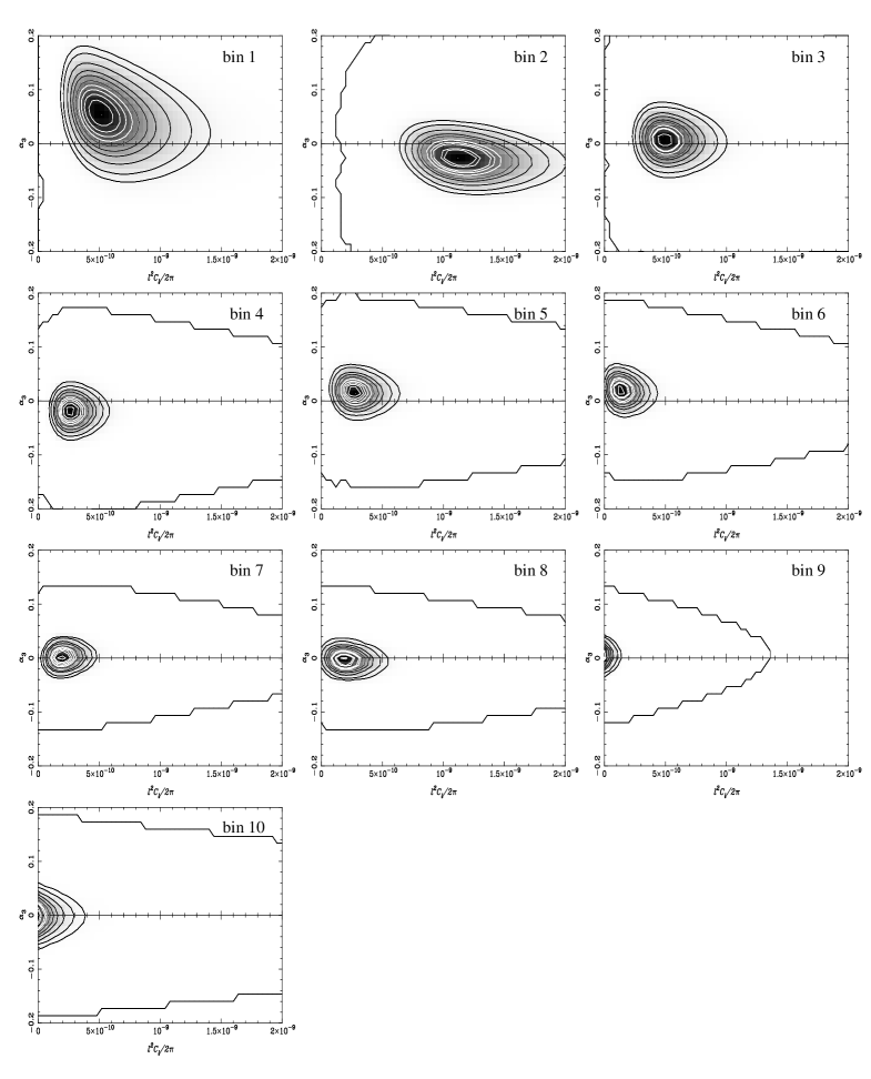
Figure 2: Confidence contours for a simulated VSA observation of a Gaussian CMB realisation drawn from a standard inflationary model. In each spectral bin the fluctuations are parametrized by the average value of $l^{2}C_{l}/(2\pi)$ and the generalised cumulant $\alpha_{3}$. Contours are at 10,20,30,…90 and 95 per cent confidence levels.

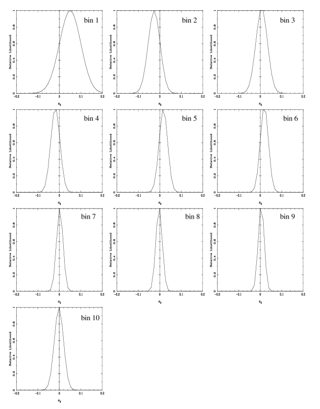
Figure 4: Marginalised likelihood functions for $\alpha_{3}$ in each spectral bin obtained from the simulated VSA observation.

Figure 6: Solid line: marginalized distribution for CMB fluctuations parameterized by $l^{2}C_{l}/(2\pi)$, for a simulated VSA observation; dashed line: conditional distribution for $\alpha_{3}=0$.

Figure 8: The joint likelihood for $\alpha_{3}$ obtained by multiplying the individual likelihoods in $\alpha_{3}$ for the 10 spectral bins.

Figure 10: The distribution of the peak of the likelihood in $\alpha_{3}$ for simulated VSA observations of several Gaussian CMB realizations.

References

- Albrecht & Steinhardt 1982 Albrecht A., Steinhardt P., 1982, Phys. Rev. Lett., 48, 1220
- Banday, Zaroubi & Górski 1999 Banday A.J., Zaroubi S., Górski K.M., 1999, ApJ, 533, 575
- Barreiro et al. 2000 Barreiro R. et al., astro-ph/0004202.
- Bernardis et al. 2000 Bernardis P. et al., 2000, Nature, 404, 995
- Bond 1995 Bond J. Richard, 1995, Phys. Rev. Lett., 74, 4369
- Bond, Jaffe & Knox 1998 Bond J. R., Jaffe A. H., Knox L., 1998, Phys. Rev., D57, 2117
- Contaldi 2000 Contaldi C., astro-ph/0005115.
- Contaldi, Bean & Magueijo 1999 Contaldi C., Bean R., Magueijo J., 1999, Phys. Lett., B468, 189
- Contaldi et al. 2000 Contaldi C. R. et al., 2000, ApJ, 534, 25
- Dodelson & Knox 2000 Dodelson S., Knox L., 2000, Phys. Rev. Lett., 84, 3523
- Ferreira, Magueijo & Górski 1998 Ferreira P.G., Magueijo J.,Górski K.M.G., 1998, ApJ, 503, L1
- Gradshteyn & Ryzhik 1996 Gradshteyn I. S., Ryzhik I. M., Table of Integrals, Series, and Products, Academic Press, 1996
- Guth 1981 Guth A. H., 1981, Phys. Rev., D23, 347
- Halliwell & Hawking 1985 Halliwell J.J., Hawking S. W., 1985, Phys. Rev. D 31, 1777
- Hanany et al. 2000 Hanany S.et al., 2000, ApJ Lett., astro-ph/0005123
- Hartle & Hawking 1983 Hartle J. B., Hawking S. W., 1983, Phys. Rev., D28, 2960
- Hobson, Lasenby & Jones 1995 Hobson M. P., Lasenby A. N., Jones M., 1995, MNRAS, 275, 863
- Kendall & Stuart 1977 Kendall M.G. and Stuart A., The Advanced Theory of Statistics, Charles Griffin, 1977
- Kogut et al. 1996 Kogut A. et al., 1996, ApJ, 464 L29
- Kogut et al. 1996 Kogut A. et al., 1996, ApJ, 464, L5
- Linde 1982 Linde A., 1982, Phys. Lett., B 108, 1220
- Linde 1983 Linde A., 1983, Phys. Lett., B 129, 177
- Linde & Mukhanov 1997 Linde A., Mukhanov V., 1997, Phys. Rev., D56, 535
- Magueijo 2000 Magueijo J., 2000, ApJ Lett., 528, L57
- Melchiorri et al. 2000 Melchiorri A. et al., 2000, ApJ Lett., 536, L-59
- Merzbacher 1970 Merzbacher E., Quantum Mechanics, Wiley, NY, 1970
- Miller et al. 1999 Miller A.D. et al., 1999, ApJ Lett., 524, L1
- Peebles 1998 Peebles P. J. E., astro-ph/9805194; astro-ph/9805212
- Pando, Valls-Gabaud & Fang 1998 Pando J., Valls-Gabaud, Fang L.Z., 1998, Phys. Rev. Lett., 81, 4568
- Salopek 1992 Salopek, D. S., 1992, Phys. Rev. D45, 1139
- Tegmark, Taylor & Heavens 1997 Tegmark Max, Taylor Andy N., Heavens Alan F., 1997, ApJ, 480, 22
- Vilenkin 1982 Vilenkin A., 1982, Phys. Lett., B 117, 25