Binary quasars

Abstract

Quasar pairs are either physically distinct binary quasars or the result of gravitational lensing. The majority of known pairs are in fact lenses, with a few confirmed as binaries, leaving a population of objects that have not yet been successfully classified. Building on the arguments of Kochanek, Falco & Muñoz (1999a), it is shown that there are no objective reasons to reject the binary interpretation for most of these. In particular, the similarity of the spectra of the quasar pairs appears to be an artifact of the generic nature of quasar spectra. The two ambiguous pairs discovered as part of the Large Bright Quasar Survey (Q 1429$-$053 and Q 2153$-$0256) are analysed using principle components analysis, which shows that their spectral similarities are not greater than expected for a randomly chosen pair of quasars from the survey. The assumption of the binary hypothesis allows the dynamics, time-scales and separation distribution of binary quasars to be investigated and constrained. The most plausible model is that the quasars’ activity is triggered by tidal interactions in a galatic merger, but that the (re-)activation of the galactic nuclei occurs quite late in the interaction, when the nuclei are within $80\pm 30$ kpc of each other. A simple dynamical friction model for the decaying orbits reproduces the observed distribution of projected separations, but the decay time inferred is comparable to a Hubble time. Hence it is predicted that binary quasars are only observable as such in the early stages of galactic collisions, after which the quiescent super-massive black holes orbit in the merger remnant for some time.

1 Introduction

A small fraction ($\sim 1$ in 1000) of quasars are observed to have at least one nearby quasar image with essentially the same redshift (e.g. Kochanek 1995; Hewett et al. 1998), and approximately 50 such systems are known in all (e.g. Keeton & Kochanek 1996). Some of the pairs (and all of the higher multiples) are the result of gravitational lensing by intervening mass distributions; some are physically distinct binary quasars. In most cases the correct interpretation is quite clear, even if considerable observational effort was required, but there is a small number ($\sim 20$) of pairs of quasars which cannot be categorised with certainty (e.g. Schneider 1993; Kochanek, Falco & Muñoz 1999a; Peng et al. 1999). These tend to have angular separations of $\ga 3$ arcsec, and in most cases are treated as potential ‘wide separation’ lenses (e.g. Narayan & White 1988; Wambsganss et al. 1995; Mortlock, Webster & Hewett 1996; Park & Gott 1997; Williams 1997). If they are lenses they indicate the presence of a significant and otherwise unknown population of dark objects with the mass of groups or clusters of galaxies (e.g. Kochanek 1995; Hawkins 1997). If they are binaries they are almost certainly the result of enhanced fuelling in galactic mergers or interactions (Djorgovski 1991; Kochanek et al. 1999a).

The arguments in support of both possibilities are summarised in Sec. 2. In Sec. 3 principal components analysis is used to objectively test the spectral similarity of several quasar pairs. The binary hypothesis is subsequently adopted for the entire pair population, and the implications for the dynamics of binary quasars are explored in Sec. 4. The conclusions are summarised in Sec. 5, together with a discussion of the future observational and theoretical possibilities.

2 Known quasar pairs

Table 1: Possible binary quasars.

Name	Status	Type	$\Delta m$	$z$	$|\Delta v_{||}|$	$\Delta\theta$		$R$		Ref.
							$\Omega_{\mathrm{m}_{0}}=1$	$\!\!\Omega_{\mathrm{m}_{0}}=0.3\!\!$	$\Omega_{\mathrm{m}_{0}}=0.3$
							$\Omega_{\Lambda_{0}}=0$	$\!\!\Omega_{\Lambda_{0}}=0\!\!$	$\Omega_{\Lambda_{0}}=0.7$
MG 0023+171	Binary?	$O^{2}R^{2}$	1.2	0.95	$170\pm 150$ km s-1	4$\aas@@fstack{\prime\prime}$8	29 kpc	34 kpc	38 kpc	1
Q 0101.8$-$3012	Unknown	$O^{2}$	0.8	0.89	$0\pm 200$ km s-1	17$\aas@@fstack{\prime\prime}$0	101 kpc	117 kpc	132 kpc	2
Q 0151+0448	Binary?	$O^{2}$	3.6	1.91	$520\pm 160$ km s-1	3$\aas@@fstack{\prime\prime}$3	19 kpc	25 kpc	28 kpc	3
QJ 0240$-$343	Unknown	$O^{2}$	0.8	1.41	$250\pm 180$ km s-1	6$\aas@@fstack{\prime\prime}$1	37 kpc	46 kpc	52 kpc	4
Q 1120+0195	Unknown	$O^{2}$	4.6	1.47	$200\pm 100$ km s-1	6$\aas@@fstack{\prime\prime}$5	40 kpc	49 kpc	55 kpc	5
PKS 1145$-$071	Binary	$O^{2}R$	0.8	1.45	$80\pm 60$ km s-1	4$\aas@@fstack{\prime\prime}$2	26 kpc	32 kpc	35 kpc	6
Q 1208+1011	Lens?	$O^{2}$	1.5	3.80	$1200\pm 1200$ km s-1	0$\aas@@fstack{\prime\prime}$5	2 kpc	3 kpc	3 kpc	7
HS 1216+5032	Binary	$O^{2}R$	1.8	1.45	$260\pm 1000$ km s-1	9$\aas@@fstack{\prime\prime}$1	56 kpc	69 kpc	77 kpc	8
Q 1343+2640	Binary	$O^{2}R$	0.1	2.03	$200\pm 900$ km s-1	9$\aas@@fstack{\prime\prime}$5	55 kpc	72 kpc	79 kpc	9
Q 1429$-$0053	Unknown	$O^{2}$	3.1	2.08	$260\pm 300$ km s-1	5$\aas@@fstack{\prime\prime}$1	30 kpc	39 kpc	42 kpc	10
Q 1634+267	Unknown	$O^{2}$	1.6	1.96	$30\pm 90$ km s-1	3$\aas@@fstack{\prime\prime}$8	22 kpc	29 kpc	32 kpc	11
J 1643+3156	Binary	$O^{2}R$	0.6	0.59	$80\pm 10$ km s-1	2$\aas@@fstack{\prime\prime}$3	12 kpc	14 kpc	16 kpc	12
Q 2138$-$431	Unknown	$O^{2}$	1.2	1.64	$0\pm 100$ km s-1	4$\aas@@fstack{\prime\prime}$5	27 kpc	34 kpc	38 kpc	13
Q 2153$-$2056	Binary?	$O^{2}$	3.4	1.85	$1100\pm 1500$ km s-1	7$\aas@@fstack{\prime\prime}$8	46 kpc	60 kpc	66 kpc	14
MGC 2214+3550	Binary	$O^{2}R$	0.5	0.88	$150\pm 400$ km s-1	3$\aas@@fstack{\prime\prime}$0	18 kpc	21 kpc	23 kpc	15
Q 2345+007	Lens?	$O^{2}$	1.5	2.15	$480\pm 500$ km s-1	7$\aas@@fstack{\prime\prime}$3	42 kpc	56 kpc	61 kpc	16

‘Status’ summarises the current evidence concerning the nature of each pair (See Sec. 2.1 for the classification criteria, and Mortlock (1999) for a summary of the evidence pertaining to each pair.); confirmed lenses are not included. ‘Type’ summarises the detected optical and radio emission of the pair using the notation of Kochanek et al. (1999a), where $O^{2}R^{2}$ denotes a pair in which both components are detected in the radio (and optical); $O^{2}R$ denotes a pair with only one radio-loud component (which is hence a binary quasar); and $O^{2}$ denotes a pair with no radio emission at all. $\Delta m$ is the magnitude difference of each pair (in the optical); $z$ is the redshift; $|\Delta v_{||}|$ is the observed line-of-sight velocity difference; $\Delta\theta$ is the angular separation of the two components; and $R$ is the projected physical separation of the two quasars, given for the three cosmological models described in Sec. 4.1.1, with $H_{0}=70$ km s^-1 Mpc^-1 assumed throughout.

References: 1. Hewitt et al. (1987); 2. Boyle et al. (1998); 3. Meylan et al. (1990); 4. Tinney (1995); 5. Meylan & Djorgovski (1988, 1989); 6. Meylan et al. (1987) and Djorgovski et al. (1987); 7. Magain et al. (1992) and Maoz et al. (1992); 8. Hagen et al. (1996); 9. Crampton et al. (1988); 10. Hewett et al. (1989); 11. Djorgovski & Spinrad (1984); 12. Brotherton et al. (1999); 13. Hawkins et al. (1997); 14. Hewett et al. (1998); 15. Muñoz et al. (1998); 16. Weedman et al. (1982).

Table LABEL:table:binaries lists all known quasar pairs which have not been confirmed as gravitational lenses, in order of increasing right ascension. This list has been compiled mainly from previous lens candidate compilations (Turner 1988; Surdej 1990a,b; Surdej et al. 1991; Surdej 1991; Schneider, Ehlers & Falco 1992; Surdej & Soucail 1993; Schneider 1993; Keeton & Kochanek 1996; Kochanek et al. 1999a), but also includes more recent discoveries, such as Q 0101.8$-$3012 [Boyle et al. 1998] and the small separation pair Q 1208+1011 (Magain et al. 1992; Maoz et al. 1992). The criteria by which these pairs are given their tentative classifications are discussed in Sec. 2.1, and a detailed summary of the status of each pair is given in Mortlock [Mortlock 1999]. Some statistical arguments relating only to the overall properties of the population of pairs are presented in Sec. 2.2.

2.1 Classification criteria

From the discovery of the first gravitational lens (Walsh, Carswell & Weymann 1979) and the subsequent interest in lensed quasars, it was soon realised that reasonably objective criteria must be established to determine whether pairs were lenses (e.g. Webster & Fitchett 1986; Schneider et al. 1992; Kochanek 1993; Kochanek et al. 1999a).

A pair can only be positively confirmed as a binary if the spectra of the images are vastly different, if only one image is radio-loud (i.e. an ‘$O^{2}R$’ pair, in the notation of Kochanek et al. 1999a), or if the quasars’ host are detected. The only necessary condition a binary must satisfy is that its components’ spectra not be ‘too similar’ to each other, the meaning of which is investigated further in Secs. 2.2 and 3.

The main sufficient conditions for a pair to be identified as a lens are: the presence of more than two images; the measurement of a time-delay between the images; or the detection of a plausible deflector. Naively, both a sufficient and necessary condition for a pair to be a lens is that its components’ spectra are identical, as gravitational lensing is achromatic. However the difficulty in assessing just how similar two spectra are, combined with the generic nature of quasar spectra, means that it is difficult to prove a pair is not a binary on these grounds, as discussed further in Sec. 3. Spectral similarity is not a necessary condition either – the light from a lensed quasar travels along different lines-of-sight to the observer, which can result in a number of achromatic effects. Dust along one line-of-sight can redden individual images (e.g. Falco et al. 1999); microlensing by stellar-mass objects can magnify the continuum of one image relative to the emission lines; intrinsic variability coupled with the time-delay can result in the simultaneous spectra of components differing; and even the fact that the light that makes up each image comes from slightly different points in the quasar can result in different spectra being observed. Further, the images of a lensed quasar can even yield different redshifts – the two components of Q 0957+561 have redshifts which differ by $\Delta z=0.0023\pm 0.00017$ [Wills & Wills 1980].

Clearly the ambiguous quasar pairs do not satisfy any of these sufficient conditions, although some come close. The generic uncertain pair has no visible deflector, but qualitatively similar spectra, neither of which allows a definite classification.

2.2 The population of pairs

If the 11 ambiguous pairs in Table LABEL:table:binaries are predominantly lenses, the statistical properties of the sample should match those of the confirmed lenses, and likewise if they are mainly binaries. Their are some potential pit-falls to this approach (e.g. the definition of the samples; the presence of recently discovered pairs, such as Q 0101.8$-$3012, which may not require the existence of a particularly dark lens) but it is a potentially powerful method.

Kochanek et al. [Kochanek et al. 1999a] used this technique to argue that most of the wide separation (i.e. $\Delta\theta\ga 3$ arcsec) pairs are not lenses for the following reasons. The existence of the $O^{2}R$ binaries, combined with the knowledge that most quasars are radio-quiet, implies a comparable or larger population of $O^{2}$ binaries – presumably the majority of the 10 in Table LABEL:table:binaries. The distribution of the ambiguous pairs’ redshifts is significantly different to that of the confirmed lenses, which is very difficult to account for in terms of lensing (e.g. Williams 1997). The distribution of flux ratios of the pairs and of the confirmed two-image lenses differ greatly (Fig. 1), although neither are consistent with the distribution predicted by a simple, spherical lens model, implying that further investigation is warranted. Lastly, if the pairs are lenses, the absence of a smooth fall-off at larger separations is at odds with most theoretical models that predict wide separation lenses (e.g. Narayan & White 1988; Kochanek 1995).

Figure 1: A cumulative plot of the magnitude differences, $\Delta m$, between the possible lensed quasar pairs (dashed line), and all known two-image lenses, both with (upper solid line) and without (lower solid line) the known arcs and rings (which are generally treated as having $\Delta m=0$). The two smooth solid curves show the distribution predicted by a simple lensing model for survey magnitude limits of $B=19$ (upper line) and $B=21$ (lower line).

The statistical objections to the binary hypothesis have been the uncanny similarities of pairs’ spectra (which is addressed in Sec. 3) and the high number of pairs at such small separations (relative to the predictions of the generic quasar-quasar correlation function). However, Kochanek et al. [Kochanek et al. 1999a] showed that the number of pairs observed was consistent with the number expected from the observed small-scale quasar-galaxy correlation function. Further implications of this are explored in Sec. 4.

3 Spectral similarities of quasar pairs

The spectra of many of the pairs do appear unusually alike, but, before this can be regarded as an objection to the binary hypothesis, it must be shown quantitatively that they are significantly more alike than those of randomly chosen quasars. There have been several attempts to implement this sort of test, but the limitations of the data have proved critical in most cases. Turner et al. [Turner et al. 1988] found that the the emission line shapes of Q 1634+267 A and B were more similar to each other than they were to those of another quasar of comparable luminosity and redshift, although the use of only a single comparison object limited the strength of the conclusions. Peng et al. [Peng et al. 1999] found that the C iv equivalent widths and continuum slopes of 14 pairs (all those in Table LABEL:table:binaries bar Q 0101.8$-$3012 and Q 1208+1011) were more alike than over 97 per cent of comparable random quasar samples, implying that the apparent spectral similarities are real. Lastly, Hawkins [Hawkins 1997] found that the colours of the two components of Q 2138$-$431 and Q 2345+007 were closer than expected, when compared to those of $\sim 10$ other quasars with similar redshifts. However the control quasars represent a heterogeneous sample, which can only increase the relative similarity of the pairs’ colours. This illustrates why such relative tests are better at demonstrating pairs can be binary objects. In a related investigation, Small et al. [Small et al. 1997] showed that the differences between the component spectra of Q 1634+267 and Q 2345+007 were no larger than the temporal variations in other quasars. Hence these pairs are consistent with being lenses, despite the differences in their spectra. However this represents only a necessary condition, and is not a sufficient condition for the lensing interpretation. The choice of experiment is probably an artifact the greater interest in finding lenses.

The analysis that follows is directed towards determining whether the two ambiguous quasar pairs in the Large Bright Quasar Survey (LBQS) are consistent with being binaries. The data is described in Sec. 3.1 and the method of comparison discussed in Sec. 3.2. The results and interpretation are given in Sec. 3.3.

3.1 Quasar pairs in the Large Bright Quasar Survey

Table 2: Quasar pairs in the LBQS.

Name	Status	$m_{\rm A}$	$m_{\rm B}$	$\Delta m$	$z$	$|\Delta v_{||}|$	$\Delta\theta$	Ref.
Q 1009$-$0252	Lens	$V=17.9$	$V=20.5$	2.6	2.74	$150\pm 200$ km s-1	1$\aas@@fstack{\prime\prime}$5	1
Q 1429$-$0053	Unknown	$R=17.7$	$R=20.8$	3.1	2.08	$260\pm 300$ km s-1	5$\aas@@fstack{\prime\prime}$1	2
Q 2153$-$2056	Binary?	$B=17.9$	$B=21.3$	3.4	1.85	$1100\pm 1500$ km s-1	7$\aas@@fstack{\prime\prime}$8	3

‘Status’ summarises the current evidence concerning the nature of each pair (See Table LABEL:table:binaries and Sec. 2.1.); $m_{\rm A}$ and $m_{\rm B}$ are the magnitudes of the primary and its companion, respectively, and $\Delta m$ is the difference between the two (The band is given in the table.); $z$ is the redshift of the pair; $|\Delta v_{||}|$ is the observed line-of-sight-velocity difference; and $\Delta\theta$ is the angular separation of the two components.

References: 1. Hewett et al. (1994); 2. Hewett et al. (1989); 3. Hewett et al. (1998).

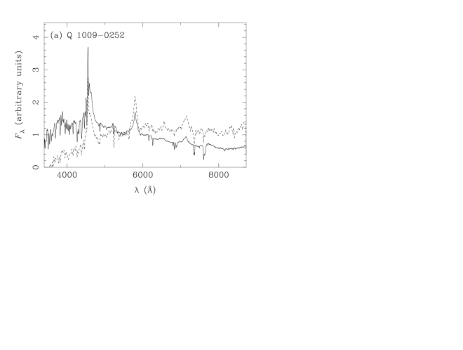
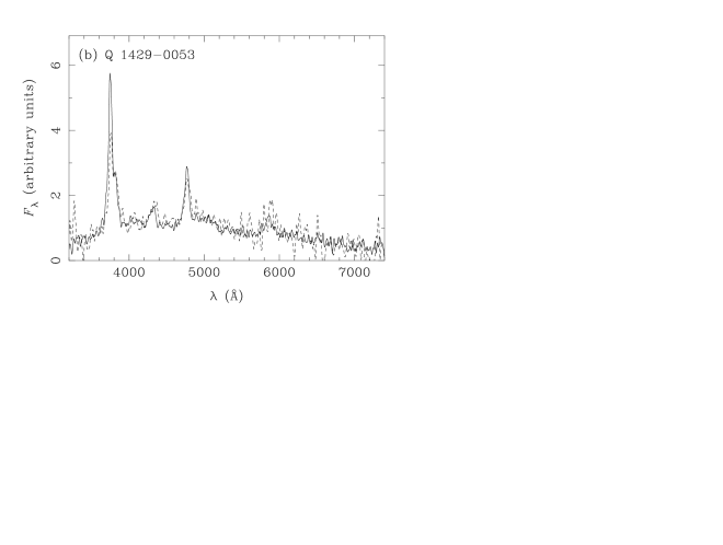
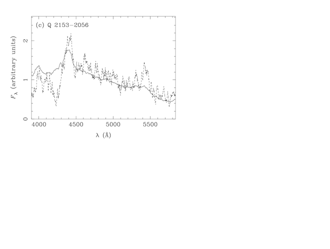
Figure 2: The spectra of the primaries (solid lines) and companions (dashed lines) of the three quasar pairs in the LBQS: Q 1009$-$0252 (a); Q 1429$-$0053 (b); and Q 2153$-$2056 (c). In each case, both spectra have been smoothed (with a smoothing length between 5 and 10 Å) and normalised to have an average flux of unity, to aid in the comparison. Note that all spectra are in the observed frame, not the rest frame.

The LBQS is a sample of 1055 quasars with $m_{B_{\mathrm{J}}}\ga 18.5$, selected spectroscopically and without any reference to morphology (Hewett, Foltz & Chaffee 1995). Due to both its size and its well-characterised selection effects, it is an excellent source of data for studying the similarities and differences between quasar spectra.

As part of the survey, there was a systematic search for companions within $\sim 10$ arcsec of each quasar. The companion search has sufficient dynamic range ($\Delta m\simeq 3.5$) to easily pick out most secondary lensed images, and also to detect potentially dimmer binary companions. The search has yielded three pairs so far (listed in Table LABEL:table:lbqs), and it is ‘unlikely that further pairs will be identified’ [Hewett et al. 1998]. Q 1009$-$0252 [Hewett et al. 1994] is a confirmed lens; Q 1429$-$0053 [Hewett et al. 1989] is a reasonable lens candidate; and Q 2153$-$2056 [Hewett et al. 1998] is probably a binary quasar. The spectra of all three pairs, taken concurrently in each case, are shown in Fig. 2, and it is clear that there are significant differences between the primary and companion of both Q 1009$-$0252 (the lens) and Q 2153$-$2056. However, a more quantitative, and hence objective, means of testing the similarity of the spectra is needed to proceed further.

3.2 Comparison of quasar spectra

The most common method of analysing spectra (aside from visual inspection) is to measure the properties of individual features, such as emission lines and continuum properties. The weakness of this approach is that the classification of the features is usually subjective at some level.

It is preferable to use a completely quantitative method, such as principal components analysis (PCA; Whitney 1983; Murtagh & Hecht 1987; Mittaz, Penston & Snijders 1990). PCA can be used on pre-determined features, but, for the reasons given above, it is more powerful to perform PCA on the raw spectra. This ‘spectral’ PCA has the advantages that it is a completely objective analysis, uses all the available data, and is adept at dealing with low signal-to-noise ratio spectra. With each spectrum treated as a vector in a multi-dimensional space, the sample of spectra represents a distribution in this space, the centroid of which is the mean spectrum. Subtracting the mean from each spectrum yields a set of points (centred on the origin) which represents the variation between spectra. The vector (or spectrum, of sorts) along which this distribution is most elongated is the first principle component (PC) of the sample. Subtracting it from all the already mean-subtracted spectra allows the procedure to be repeated, generating the subsequent components. The subtraction of only the first few PCs usually (i.e. if the PCA is successful) leaves a condensed, spherical distribution of points that is essentially a hyper-sphere of noise. Almost all the information is contained the in the first few components; the data compression involved can be large. Francis et al. [Francis et al. 1992] found that the LBQS spectra could be expressed in terms of coefficients of $\sim 10$ components, as opposed to several hundred wavelength bins.

Following Francis et al. [Francis et al. 1992], two subsets were taken from the LBQS for the PCA. Sample 1 contains 325 quasars (including all three pairs) with $1.4\leq z\leq 2.7$, and rest-frame spectra covering the range from 1400 Å to 2200 Å. Importantly, this range covers several prominent emission lines, notably C iv (1549 Å) and Al iii/C iii] (1858 Å/1909 Å). Sample 2 has only 209 quasars (including the the lens and the wide separation pair Q 1429$-$0053), but, with $1.8\leq z\leq 3.3$, covers a sligtly bluer part of rest-frame spectrum: 1180 Å to 1780 Å. It includes the C iv emission line and the Ly $\alpha$/N v complex (1216 Å/1240 Å). The other wide separation pair, Q 2153$-$2056, could not be included in sample 2, as the available spectra (Fig. 2 (c)) do not include the Ly $\alpha$/N v blend. A number of quasars, including the stated pairs, appear in both samples.

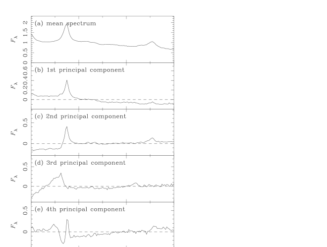
Figure 3: The mean spectrum (a) and the first four component ‘spectra’ (b-e) of sample 1, plotted as a function of rest-frame (i.e. in the frame of the quasars) wavelength. The mean spectrum is normalised to an average flux of unity, and all the principal components have zero mean. The 3rd and 4th PCs have been inverted so that emission features are positive. The prominent emission lines are C iv (at $\sim 1550$ Å) and the Al iii/C iii] blend (at $\sim 1900$ Å).

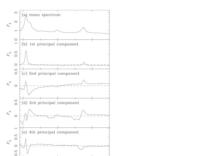
Figure 4: The mean spectrum (a) and the first four component ‘spectra’ (b-e) of sample 2, plotted as a function of rest-frame (i.e. in the frame of the quasars) wavelength. The mean spectrum is normalised to an average flux of unity, and all the principal components have zero mean. The 3rd and 4th PCs have been inverted so that emission features are positive. The prominent emission lines are the Ly $\alpha$/N v blend (at $\sim 1230$ Å) and C iv (at $\sim 1550$ Å).

Spectral PCA was performed on both subsamples, generating a set of PC spectra for each sample, and a set of coefficients for each quasar. As expected, most of the variation between spectra was contained in the first few components, which are shown in Fig. 3 (for sample 1), and Fig. 4 (for sample 2). The components are similar to those shown in Francis et al. [Francis et al. 1992] (as expected, given the related set of input spectra), and their interpretation is also similar. The first three components of both samples are related to: the cores of the emission lines (PC 1; Figs. 3 and 4 (b)); the continuum slope (PC 2; Figs. 3 and 4 (c)); and broad absorption lines (PC 3; Figs. 3 and 4 (d)). The 4th PC of samples 1 and 2 relate to the wings of of the C iv and Ly $\alpha$ emission lines, respectively (Figs. 3 and 4 (e)). It is promising that the C iv line is prominent in the first PC, as it is the most prominent difference between the spectra of several of the confirmed binaries (Q 1216+5032 and Q 1343+2640), and both Turner et al. [Turner 1988] and Peng et al. [Peng et al. 1999] found its properties revealing.

Whilst the PCA has enabled each spectrum to be specified in terms of several numbers (i.e. the coefficients of the first few PCs), each spectrum is still a multi-dimensional vector. The data can be further compressed by defining a metric in the PC space. The PCA naturally scales the variance in each component with its relative importance, so a simple Euclidean metric is chosen. The difference, $D$, between the spectra of two quasars A and B is then given by

$$D_{\mathrm{A}B}=\left[\sum_{n=1}^{n_{\mathrm{m}ax}}(C_{{\mathrm{A}},n}-C_{{\mathrm{B}},n})^{2}\right]^{1/2},$$ (1)

where $C_{{\mathrm{A}},n}$ and $C_{{\mathrm{B}},n}$ are the coefficients of the $n$th principal component of spectra of A and B, respectively, and $n_{\mathrm{m}ax}$ is the highest component used. The latter does not have an appreciable affect on the results, as long as the first few components are included, so $n_{\mathrm{m}ax}=4$ was used.

Two sets of $D$-values were created for each sample: the differences between all the spectra in the sample; and the differences between each of the pairs’ primaries and the rest of the sample (which determines the fraction of spectra in the sample that are closer to the primary in question than its companion). The resultant cumulative plots are shown for sample 1 and sample 2 in Figs. 5 and 6, respectively.

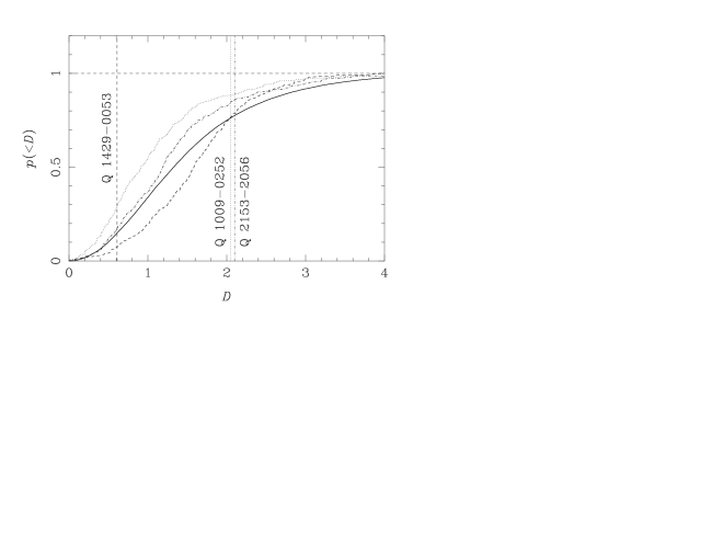
Figure 5: The cumulative distribution of the difference between two spectra, $D$, shown for sample 1 (Sec. 3.2). The solid line is the distribution derived from all possible pairs of spectra in the sample; the other lines are from the differences between each of the primaries of the three pairs (Q 1429$-$0053: dashed line; Q 2153$-$2056: dot-dashed line; Q 1009$-$0252: dotted line) and the rest of the sample. The three vertical lines show difference between each primary and its respective companion.

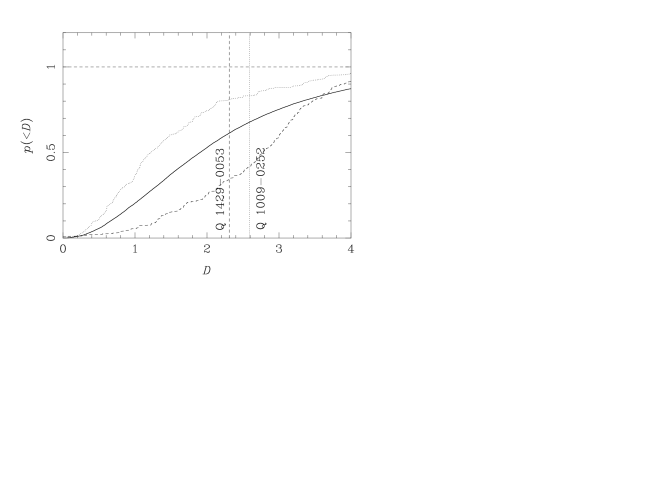
Figure 6: The cumulative distribution of the difference between two spectra, $D$, shown for sample 2 (Sec. 3.2). The solid line is the distribution derived from all possible pairs of spectra in the sample; the other lines are from the differences between each of the primaries of the two pairs (Q 1429$-$0053: dashed line; Q 1009$-$0252: dotted line) and the rest of the sample. The two vertical lines show difference between each primary and its respective companion.

3.3 Implications for the quasar pairs

The two components of the confirmed lens, Q 1009$-$0252, are clearly different. This is not unexpected – as discussed in Sec. 2.1, there are a number of reasons why lensed spectra need not be the same. However, this analysis shows that they can actually be less similar than a two spectra chosen at random: Fig. 5 shows that 75 per cent of random pairs are more alike than the components of the lens. However the main difference between the two spectra of the Q 1009$-$0252 is the reddening of the companion spectrum (Fig. 2 (a)), which is probably due to dust along the line-of-sight to the fainter image (see Sec. 2.1 and Falco et al. 1999).

The components of Q 2153$-$2056 are also more dissimilar than those of random pairs. Naively, the lesson of Q 1009$-$0252 implies that Q 2153$-$2056 cannot be rejected as a lens on this basis alone. The difference between the spectra of Q 2153$-$2056 cannot be so readily explained in terms of lensing – indeed it appears that the companion is a broad absorption line quasar, which is only explained simply if they are two distinct objects. This distinction reveals one of the limitations of PCA – there is no physics or plausibility input, and so it cannot tell that some spectral differences (specifically Q 1009$-$0252) might be due to dust. In this instance, a continuum fit to the spectra would circumvent this problem. Due to both the spectral differences and the absence of a visible deflector, Hewett et al. [Hewett et al. 1998] interpret Q 2153$-$2056 as a probable binary, a conclusion which is confirmed here.

The results for Q 1429$-$0053 (which is a more probable lens a priori) are more interesting. For the wavelength range covered by sample 1, the components of Q 1429$-$0053 are more similar than $\sim 85$ per cent of random pairs. It also appears that Q 1429$-$0053 is a slightly unusual quasar spectrally, and so only $\sim 9$ per cent of the spectra are more similar to the primary than its companion. The sample 2 results paint a slightly different picture. Q 1429$-$0053 B is no more similar to Q 1429$-$0053 A than a random quasar from the sample. This is despite the fact that Q 1429$-$0053 A is at least slightly unusual – the dashed line and the solid line (representing the whole sample) are quite separated in Fig. 6. Such results are perfectly consistent with Q 1429$-$0053 being a lens (c.f. Q 1009$-$0252), but are also perfectly consistent with the two spectra having been drawn at random from the LBQS, and hence consistent with Q 1429$-$0053 being two distinct quasars. However, almost all the difference between the two components of Q 1429$-$0053 can be attributed to the relative strengths of the Ly $\alpha$-N v complex (appearing at $\sim 4800$ Å in Fig. 2 (b)), the equivalent widths differ by $\sim 50$ per cent. The possibility of microlensing of the the secondary image (See Sec. 2.1.) means that the lens interpretation is still possible, although the macrolensing flux ratio this would imply ($\Delta m\simeq 3.5$) is very unlikely a priori (e.g. Fig. 1).

There are several potential systematic errors which, whilst they do not affect the above conclusions, are important in principle. The samples covered a wide redshift range, possibly increasing the spread in the samples’ spectra; this could result in a true binary being rejected, but could not result in a lens being wrongly classed a binary. Another potential bias that is unimportant is the faintness of the companion images in these pairs – lower luminosity quasars might have different spectra. If the pairs are lenses this is clearly irrelevant, as they are not intrinsically so faint. If they are binaries, any bias that might make the spectra appear more dissimilar is acceptable, even desirable.

The main source of random uncertainty is the low quality of the companions’ spectra (despite the fact that PCA is adept at analysing low signal-to-noise data), which is simply a function of their faintness (Table LABEL:table:lbqs). Several hours’ observation on a 10-m class telescope would yield companion spectra of better quality than the current primary spectra.

On the basis of these results and the existing work summarised in Sec. 2, all the ambiguous pairs are assumed to be binaries in Sec. 4. This, however, is quite an adventurous extrapolation – the broader but less rigorous results of Peng et al. [Peng et al. 1999] imply that the spectra of the pair population are unusually alike.

4 Dynamics of binary quasars

If all the quasar pairs listed in Table LABEL:table:binaries are physical binaries, there are far too many to represent a simple a small-scale manifestation of quasar clustering [Djorgovski 1991]. The fairly natural conclusion (Djorgovski 1991; Schneider 1993) is that any close quasar pairs are the result of increased nuclear activity in interacting galaxies. Kochanek et al. [Kochanek et al. 1999a] showed that the number of binaries matches the number expected from the quasar-galaxy correlation function at small scales. Henceforth, all the pairs in Table LABEL:table:binaries are treated as physical binaries, and the merger model is also adopted. The sample of pairs can then be used to constrain the distribution of physical separations (Sec. 4.1), and also to investigate the formation and evolution of binary quasars (Sec. 4.2).

4.1 Physical separations

The projected separations of the quasar pairs can be inferred for a given cosmological model (Sec. 4.1.1), but some method of inversion is required to obtain the distribution of physical separations. A random deprojection is explored in Sec. 4.1.2 and a simple orbital model is discussed in Sec. 4.1.3.

4.1.1 Cosmological models

The projected separations of the pairs are given by $R=\Delta\theta\,d_{\mathrm{A}}(0,z)$, where $d_{\mathrm{A}}$ is the angular diameter distance, and so $R$ varies with the cosmological model (and also within a model, due to weak lensing). Three models are used: the Einstein-de Sitter (EdS) model ($\Omega_{\mathrm{m}_{0}}=1$ and $\Omega_{\Lambda_{0}}=0$); a low-density model ($\Omega_{\mathrm{m}_{0}}=0.3$ and $\Omega_{\Lambda_{0}}=0$); and a low-density, spatially-flat model ($\Omega_{\mathrm{m}_{0}}=0.3$ and $\Omega_{\Lambda_{0}}=0.7$), where $\Omega_{\mathrm{m}_{0}}$ is the ratio of the current density of the universe to the critical density and $\Omega_{\Lambda_{0}}$ is the similarly normalised cosmological constant (e.g. Carroll, Press & Turner 1992). The $\sim 10$ per cent error in Hubble’s constant (taken to be $H_{0}=70$ km s^-1 Mpc^-1 here) does not contribute significantly to the uncertainty in $R$.

4.1.2 Random deprojection

Figure 7: The differential (a) and cumulative (b) separation distribution of binary quasars obtained by applying the random deprojection described in Sec. 4.1.2 to the data listed in Table LABEL:table:binaries. The three lines show the results assuming the three cosmological models described in Sec. 4.1.1: the EdS model (solid line); the low density model (dashed line) and the low density, flat model (dot-dashed line).

The problem of deprojection – effectively obtaining three dimensional information from a two-dimensional image of the sky – is an old one, with a number of different partial solutions (e.g. Courant & Hilbert 1962; Gerhard & Binney 1996). The problem at hand is to obtain a probability distribution of the physical separation, ${\mathrm{d}}p/{\mathrm{d}}r|_{R}$, given an observed projected separation, $R$. A Bayesian approach is adopted whereby the separation vector, $\mn@boldsymbol{r}$, is considered to be randomly-oriented, a posteriori. Mathematically, ${\mathrm{d}}p/{\mathrm{d}}i=\sin(i)$, where $i$ is the (inclination) angle between $\mn@boldsymbol{r}$ and the line-of-sight. It is normalised for the range $0\leq i<\pi/2$, and the projected separation is given by $R=r|\sin(i)|$. From this, a change of variables yields

$$\left.\frac{{\mathrm{d}}p}{{\mathrm{d}}r}\right|_{R} = \left|\frac{{\mathrm{d}}p}{{\mathrm{d}}i}\right|\left|\frac{{\mathrm{d}}i}{{\mathrm{d}}r}\right|$$ (5)

$$= \left\{\begin{array}[]{lll}0,&{\rm if}&r<R,\\ &&\\ \frac{16}{\pi}\frac{R^{3}}{r^{4}}\sqrt{1-\frac{R^{2}}{r^{2}}},&{\mathrm{i}f}&r\geq R,\end{array}\right.$$

where the final distribution is also normalised to unity, and has an expectation value of $16/(3\pi)R$, assuming $R>0$.

Convolving ${\mathrm{d}}p/{\mathrm{d}}r|_{R}$ with the data gives an approximation to the physical separation distribution of the binary quasars, the differential and cumulative forms of which in Fig. 7. This ‘random deprojection’ shows a tail of pairs with quite large separations and a possible paucity of small separation pairs. (The one pair with $r\la 10$ kpc, Q 1208+1011 is a probable lens; if it were confirmed as such, the small separation ‘hole’ would be quite clear.) Any hole cannot explained by selection effects, as there are a large number of lenses with angular separations of $\sim 1$ arcsec, implying that any such binaries would have been found. Kochanek et al. [Kochanek et al. 1999a] showed that dynamical friction (Sec. 4.2.3) can account for the hole, although the inferred separation distribution (linearly rising with $r$) is otherwise quite different from the approximately exponential fall-off apparent in Fig. 7. Some clues as to the nature of small separation binaries might be given by the discovery of three possible binaries in a sample of $\sim 100$ BL Lacs [Scarpa et al. 1999]. The frequency of these pairs is far too high to be explained in terms of gravitational lensing by galaxies, but the binary interpretation is no more comfortable. It would require not only that a few per cent of BL Lacs are binaries, but that the optical jets of the companion BL Lacs are parallel.

4.1.3 Orbital models

Figure 8: The cumulative distribution of projected separation, $R$, for the quasar pairs in Table LABEL:table:binaries and the best-fit dynamical friction model described in Sec. 4.1.3. The three lines show the results assuming the three cosmological models described in Sec. 4.1.1: the EdS model (solid line); the low density model (dashed line) and the low density, flat model (dot-dashed line).

An approach almost opposite to the random deprojection used in Sec. 4.1.2 is to assume an orbital model for the binaries, and fit the resultant distribution of projected separations to the data. The paths of two quasars in a pair of merging galaxies is undoubtedly complex, but a natural first approximation is to assume that they are in decaying elliptical orbits. However averaging over the random orientation removes most of the effects of ellipticity, so circular orbits can be used in general [Mortlock 1999]. The main difference was in the radius of closest approach, which may be relevant to the activation of the quasars (Sec. 4.2.2). The existence of the outer cut-off of between 50 kpc and 100 kpc is confirmed, independent of the distribution of separations used. The putative inner cut-off is less well constrained, and, assuming ${\mathrm{d}}p/{\mathrm{d}}r\propto r$ (based on the dynamical friction approximation discussed in Sec. 4.2.3), the data is consistent with a population of pairs extending to zero separation, as shown in Fig. 8. However, formally better fits are obtained with an inner cut-off of $\sim 10$ kpc, especially if the smallest separation pair, Q 1208+1011, is a lens as suspected. An inner cut-off would imply that the at least one of the quasars in each pair ‘turns off’ prior to the complete decay of the orbits. Possible reasons for this are discussed in Sec. 4.2.3.

4.2 Physical processes

If binary quasars are the result of galactic collisions during which both nuclei become active, the assumption that the systems are bound implies a minimum mass for the systems (Sec. 4.2.1), and the distribution of physical separations (along with timing arguments) can be used to investigate both the activation and evolution of the pairs (Secs. 4.2.2 and 4.2.3, respectively).

4.2.1 Total energy

Figure 9: A scatter plot showing the projected separation, $R$, and the line-of-sight velocity difference, $\Delta v_{||}$, of the candidate binary quasars listed in Table LABEL:table:binaries. The velocity error bars are random measurement errors, but the separation errors are taken from the spread in $R$ over cosmological models, and are thus both random and systematic. Also shown is $E_{\mathrm{m}in}=0$ [as defined in equation (6)], if each quasar’s host galaxy weighed $10^{12}M_{\sun}$ (solid line), $5\times 10^{11}M_{\sun}$ (dashed line) or $10^{11}M_{\sun}$ (dot-dashed line). If the binaries are bound, the points should lie below the relevant line.

It is possible that quasars could form in ‘glancing’ collisions (e.g. Noguchi 1987, 1988), but the absence of ‘post-collisional’ pairs with larger separations argues against this for the binary population, implying that they exist in gravitationally bound systems. The minimum possible centre-of-mass frame energy of a pair (obtained by setting the line-of-sight separation and projected velocity difference to zero) is

$$E_{\mathrm{m}in}=\frac{M_{\mathrm{A}}M_{\mathrm{B}}}{M_{\mathrm{A}}+M_{\mathrm{B}}}\frac{\Delta v^{2}_{||}}{2}-\frac{GM_{\mathrm{A}}M_{\mathrm{B}}}{R},$$ (6)

where $G$ is Newton’s gravitational constant, and $M_{\mathrm{A}}$ and $M_{\mathrm{B}}$ are the masses associated with the two quasars. Inverting equation (6) and assuming $E_{\mathrm{m}in}=0$ gives the hard lower limit for the mass of a bound system as

$$M_{\mathrm{t}ot}=M_{\mathrm{A}}+M_{\mathrm{B}}\geq\frac{R\,\Delta v^{2}_{||}}{2G}.$$ (7)

Fig. 9 shows a scatter plot of the projected separations and velocity differences of all the pairs in Table LABEL:table:binaries, with the large uncertainties in both $R$ and $\Delta v_{||}$ clearly important. Despite this, $M_{\mathrm{t}ot}\ga 5\times 10^{11}M_{\sun}$ is inferred, confirming that quasars are typically in larger galaxies (Hooper, Impey & Foltz 1997). However using the random deprojection disussed in Sec. 4.1.2 to account for the projection effects yields a larger (but softer) limit of $M_{\mathrm{t}ot}\ga 2\times 10^{12}M_{\sun}$ [Mortlock 1999].

4.2.2 (Re-)activation

It is widely believed that quasars are the active nuclei of galaxies, where gas (and other material) accretes onto a massive central black hole (e.g. Lynden-Bell 1969; Rees 1984). Many galaxies have massive but quiescent black holes at their centres (e.g. Kormendy et al. 1996, 1997), and there are several plausible explanations for how they may begin accreting and become active galactic nuclei. One important mechanism appears to be encounters between galaxies, which can result in the formation of a massive black hole (e.g. Rees 1984) or provide fuel to previously quiescent nuclei. This is supported by Hubble Space Telescope (HST) observations which show that many quasars’ host galaxies are distorted (Bahcall, Kirhakos & Schneider 1995a; Boyce, Disney & Bleaken 1999) and that low-redshift quasars are often found to be physically associated with other galaxies (e.g. Yee 1987; Bahcall, Kirhakos & Schneider 1995b; Bahcall et al. 1997) or involved in collisions [Steidel & Sargent 1990]. $N$-body simulations also show that gravitational torques between colliding galaxies can cause gas to flow to their cores, potentially acting as fuel for the central black holes [Barnes & Hernquist 1996]. The scales of the in-flows are not great enough to produce new black holes, but are consistent with the re-fuelling model. However, the simulations only predict in-flow to within a few hundred pc of the galaxies’ cores, whereas typical quasar accretion disks extend out to only pc scales [Peterson 1997]. It is not clear whether dissipation is sufficient to allow the gas to fall further.

The formation of binary quasars is qualitatively consistent with the reactivation process, provided that the progenitors (or their central black holes) are sufficiently massive. The observational result that the activation radius is between 50 kpc and 100 kpc (Sec. 4.1) implies that quasar formation does not occur until quite late in the collision process. This is consistent with the $N$-body simulations of Barnes & Hernquist [Barnes & Hernquist 1996], which showed that gas inflows took some time to occur.

The separation scale of the binaries, together with the requirement of a massive black hole, is also suggestive of the fact that quasars form in larger galaxies. If this is the case, encounters between dwarfs and large galaxies can result in the formation of a quasar, but only collisions between two large galaxies can result in a binary quasar. The fraction of merger-related quasars which are binaries is comparable to the fraction of collisions in which both galaxies have central black holes of $\ga 10^{6}M_{\sun}$. Assuming a Schechter [Schechter 1976] mass function for the galaxies, and that $\sim 20$ per cent of those heavier than $M_{*}\simeq 10^{11}M_{\sun}$ contain large black holes [Magorrian et al. 1998], about 1 per cent of all merger-formed quasars should be in binary systems. Combined with the observation that only 1 quasar in $\sim 1000$ is a binary, this implies that about 10 per cent of quasar activity is related to galactic interactions. This is probably an underestimate of the fraction, however, as interactions between two large galaxies are almost certainly more efficient than collisions involving a dwarf galaxy. Further, if quasars all have a dusty torus which is both optically thick and subtends a large fraction of the solid angle around the central engine, both the quasars in a pair must be close to face-on for it to be observed as a binary. Extrapolating from the observation that $\sim 25$ per cent of all Seyferts are of Type I [Peterson 1997], 1 in $\sim 4$ of all quasars are visible, but only 1 in $\sim 16$ binaries are detected as such. It is thus possible that $\sim 50$ per cent of all quasars are formed during galactic interactions and collisions.

4.2.3 Evolution

The theoretical and observational evidence discussed in Sec. 4.2.2 is consistent with binary quasars forming during galactic mergers. Once the merger has begun to settle, the quasars can be treated as point-masses moving in a static, isothermal halo. Their orbits slowly decay, as they lose energy and angular momentum through dynamical friction (e.g. Binney & Tremaine 1987), eventually either merging (e.g. Makino & Ebisuzaki 1994) or forming a hard binary that lasts for a Hubble time or more (e.g. Begelman, Blandford & Rees 1980; Rajagopal & Romani 1996). If the quasars have mass $M\simeq 10^{9}M_{\sun}$ by this stage, and are in circular orbits of speed $\sqrt{2}\sigma$ (where $\sigma$ is the velocity dispersion of the halo), the time spent with separation at radius $r$ is [Binney & Tremaine 1987]

$$\left|\frac{{\mathrm{d}}t}{{\mathrm{d}}r}\right|\simeq 3.3\frac{\sigma}{GM\ln(\Lambda)}r,$$ (8)

where $\ln(\Lambda)\simeq\ln(2r_{*}\sigma^{2}/GM)$ is the Coulomb logarithm, which characterises the strength of the interaction, and $r_{*}\simeq 10$ kpc [Lacey & Cole 1993]. Hence ${\mathrm{d}}p/{\mathrm{d}}r\propto r$, as used in Sec. 4.1.3 to fit the observed separation distribution. The orbital decay proceeds at a greater rate as $r$ decreases, potentially explaining the small separation hole (Sec. 4.1).

The time-scale for the decay, $t_{\mathrm{D}F}$, is found by integrating equation (8) from $r_{\mathrm{m}ax}$ to 0. Following Binney & Tremaine [Binney & Tremaine 1987],

$$t_{\mathrm{D}F} \simeq \frac{1.65}{\ln(\Lambda)}\frac{r_{\mathrm{m}ax}^{2}\sigma}{GM}$$ (9)

$$\simeq 4\times 10^{9}\left(\frac{r_{\mathrm{m}ax}}{{\rm 20\,\,kpc}}\right)^{2}\frac{\sigma}{{\mathrm{2}00\,\,km\,\,s}^{-1}}\frac{10^{9}M_{\sun}}{M}\,\,{\rm yr},$$

where the scale values have been chosen to give the shortest plausible decay time. The dynamical time-scale of the binaries is then close to a Hubble time, and much longer than both the ‘settling’ time of the merged halo ($<10^{9}$ yr; Barnes 1992) and the expected quasar lifetime. A black hole of initial mass $\sim 10^{7}M_{\sun}$ (as implied by dynamical measurements of local galaxies; Kormendy et al. 1996) accreting at the Eddington limit [Peterson 1997] would reach $\sim 10^{10}M_{\sun}$ in much less than $10^{9}$ yr. No such massive black holes are observed now (e.g. Kormendy & Richstone 1995), so this places an upper limit on quasar masses and hence their lifetimes. Comparison of the three time-scales implies that binary quasars are short-lived, existing only whilst the host galaxies are actively merging. The most likely explanation for the death of the binaries (and other quasars in mergers) is that the in-flow of gas ceases, probably as the merger becomes more stable. Moreover, by the time the orbits decay due to dynamical friction, the merging black holes are already quiescent, and the observed binary separation distribution is a random sampling of the chaotic phase of the merger.

If the above model is correct, the hosts of binary quasars should be distinct (in the case of a ‘new-born’ binary), or, more likely, highly distorted. The host galaxies of MGC 2214+3350 A and B [Muñoz et al. 1998] have been detected by the HST, and in fact out-shine the quasars in the $H$-band [Kochanek et al. 1999b]. The galaxies show no obvious signs of being distorted, which implies both that their physical separation is considerably greater than their projected separation of $\sim 20$ kpc, and that the nuclei have only recently become active. Comparable observations – which need not be prohibitively deep – of some of the other ambiguous pairs ought to prove similarly revealing.

5 Conclusions

Djorgovski [Djorgovski 1991] and Kochanek et al. [Kochanek et al. 1999a] have both argued that most of the known wide separation quasars pairs are not the result of gravitational lensing, as summarised in Sec. 2. However, there have also been some valid objections to the interpretation of the pairs as physical binaries. The strongest was that the spectra of the pairs appear to be very similar. Sec. 3 consists of a quantitative evaluation of this claim for the three quasar pairs discovered as part of the LBQS, and shows that, despite appearances, none of these pairs can be rejected as binaries on spectral grounds. Extrapolating to the rest of the ambiguous quasar pairs, the simplest conclusion is that they are all binary quasars.

The adoption of the binary hypothesis for the entire population of 16 pairs listed in Table LABEL:table:binaries provides a significant data-set of binary quasars, and even if some do turn out to be lenses, the statistical properties of the population will not be greatly changed. Assuming quasars are the nuclei of large galaxies, the velocity differences of the pairs are consistent with them belonging to bound systems, which supports the idea that they are part of galactic mergers. Both the orbital and deprojection analyses presented in Sec. 4.1 suggest that the galactic nuclei become active at separations of between 50 kpc and 100 kpc, depending on the cosmology and the ellipticity of the quasars’ orbits. This is certainly consistent with the scales at which the tides from large galaxies become important. However the time-scales suggested for the orbits of the nuclei to decay are very large – certainly longer than the lifetime of a quasar accreting at the Eddington limit. Indeed it seems probable that the quasars remain active only whilst the host galaxies are merging, in which case most of the binaries should exist in very distorted hosts, and not in a relaxed merger. The observation that the host galaxies of MGC 2214+3550 A and B [Kochanek et al. 1999b] are undisturbed then suggests that this is a very young binary.

Whilst it is clear that the physics of merging galaxies and active galactic nuclei are far from solved, there are also a number of questions that can be answered observationally. Further spectroscopy and radio observations of a number of the quasar pairs should reveal whether they are binaries, although there are also several which are still not classified despite major observational efforts. The nature of the ‘turn on’ radius will be more strongly constrained by the 2 degree Field quasar survey [Boyle et al. 1998], which will include analysis of the nearby companions of $\sim 3\times 10^{4}$ quasars. On a longer time-scale, the Sloan Digital Sky Survey [Gunn & Weinberg 1995] will observe $\sim 10^{5}$ quasars, and is expected to find several hundred lenses and pairs, an order of magnitude increase on the number known presently. Both the lower limits on mass of the quasars’ host galaxies and the constraints on the activation radius could be determined to within $\sim 10$ per cent from such a sample.

References

- [Bade et al. 1997] Bade, N., Siebert, J. Lopez, S., Voges, W., Reimers, D., 1997, A&A, 317, L13
- [Bahcall et al. 1995a] Bahcall, J.N., Kirhakos, S., Schneider, D.P., 1995a, ApJ, 447, L1
- [Bahcall et al. 1995b] Bahcall, J.N., Kirhakos, S., Schneider, D.P., 1995b, ApJ, 450, 486
- [Bahcall et al. 1997] Bahcall, J.N., Kirhakos, S., Saxe, D.H., Schneider, D.P., 1997, ApJ, 479, 642
- [Barnes 1992] Barnes, J.E., 1992, ApJ, 393, 484
- [Barnes & Hernquist 1996] Barnes, J.E., Hernquist, L., 1996, ApJ, 471, 115
- [Begelman et al. 1980] Begelman, M.C., Blandford, R.D., Rees, M.J., 1980, Nature, 287, 307
- [Binney & Tremaine 1987] Binney, J., Tremaine, S., 1987, Galactic Dynamics. Princeton University Press, Princeton
- [Blandford & Rees 1991] Blandford, R.D., Rees, M.J., 1991, in Holt, S.S., Neff, S.G., Urry, C.M., eds., AIP Conference Proceedings 24: Testing the AGN Paradigm. American Institute of Physics, New York, 3
- [Boroson & Green 1992] Boroson, T.A., Green, R.F., 1992, ApJS, 80, 109
- [Boyce et al. 1999] Boyce, P.J., Disney, M.J., Bleaken, D.G., 1999, MNRAS, 302, L39
- [Boyle et al. 1998] Boyle, B.J., Croom, S.M., Smith, R.J., Shanks, T., Miller, L., Loaring, N.S., 1998, Phil. Trans. R. Soc. Lond. A, 357, 185
- [Brotherton et al. 1999] Brotherton, M.S., Gregg, M.D., Becker, R.H., Laurent-Muehleisen, S.A., White, R.L., Stanford, S.A., 1999, ApJ, 514, 61
- [Carroll et al. 1992] Carroll, S.M., Press, W.H., Turner, E.L., 1992, ARA&A, 30, 499
- [Courant & Hilbert 1962] Courant, R., Hilbert, D., 1962, in Methods of Mathematical Physics Vol. 1. Interscience, New York, p. 158
- [Crampton et al. 1988] Crampton, D., Cowley, A.P., Hickson, P., Kindl, E., Wagner, R.M., Tyson, J.A., Gullixson, C., 1988, ApJ, 330, 184
- [Djorgovski 1991] Djorgovski, S., 1991, in Crampton, D., ed., ASP Conference Series Vol. 21: The Space Distribution of Quasars. Astronomical Society of the Pacific, San Francisco, p. 349
- [Djorgovski & Spinrad 1984] Djorgovski, S., Spinrad, H., 1984, ApJ, 282, L1
- [Djorgovski et al. 1987] Djorgovski, S., Perley, R., Meylan, G., McCarthy, P., 1987, ApJ, 321, L17
- [Falco et al. 1999] Falco, E.E., Impey, C.D., Kochanek, C.S., Lehár, J.A., McLeod, B.A., Rix, H.-W., Keeton, C.R., Muñoz, J.A., Peng, C.Y., 1999, ApJ, submitted
- [Francis et al. 1992] Francis, P.J., Hewett, P.C., Foltz, C.B., Chaffee, F.H., 1992, ApJ, 398, 476
- [Gerhard & Binney 1996] Gerhard, O.O., Binney, J., 1996, MNRAS, 279, 993
- [Gunn & Weinberg 1995] Gunn, J.E., Weinberg, D., 1995, in Maddox, S., Aragón-Salamanca, A., eds., Wide-Field Spectroscopy and the Distant Universe. World Scientific, Singapore, p. 3
- [Hagen et al. 1993] Hagen, H.-J., Hopp, U., Engels, D., Reimers, D., 1996, A&A, 308, L25
- [Hawkins 1997] Hawkins, M.R.S., 1997, A&A, 328, L25
- [Hawkins et al. 1997] Hawkins, M.R.S., Clements, D., Fried, J.W., Heavens, A.F. Veron, P., Minty, E.W., van der Werf, P., 1997, MNRAS, 291, 811
- [Hewett et al. 1989] Hewett, P.C., Webster, R.L., Harding, M.E., Jedrzejewski, R.I., Foltz, C.B., Chaffee, F.H., Irwin, M.J., Le Fèvre, O., 1989, ApJ, 346, L61
- [Hewett et al. 1994] Hewett, P.C., Irwin, M.J., Foltz, C.B., Harding, M.E., Corrigan, R.T., Webster, R.L., Dinshaw, N., 1994, AJ, 108, 1534
- [Hewett et al. 1995] Hewett, P.C., Foltz, C.B., Chaffee, F.H., 1995, AJ, 109, 1498
- [Hewett et al. 1998] Hewett, P.C., Foltz, C.B., Harding, M.E., Lewis, G.F., 1998, AJ, 115, 383
- [Hewitt et al. 1987] Hewitt, J.N., et al., 1987, ApJ, 321, 706
- [Hooper et al. 1997] Hooper, E.J., Impey, C.D., Foltz, C.B., 1997, ApJ, 480, L95
- [Keeton & Kochanek 1996] Keeton, C.R., Kochanek, C.S., 1996, in Kochanek, C.S. & Hewitt, J.N., eds., Proceedings of IAU Symposium 173: Astrophysical Applications of Gravitational Lensing. Kluwer Academic Publishers, Dordrecht, p. 419
- [Kochanek 1993] Kochanek, C.S., 1993, ApJ, 417, 438
- [Kochanek 1995] Kochanek, C.S., 1995, ApJ, 453, 545
- [Kochanek et al. 1999a] Kochanek, C.S., Falco, E.E., Muñoz, J.A., 1999a, ApJ, 510, 590
- [Kochanek et al. 1999b] Kochanek, C.S., Falco, E.E., Impey, C.D., Lehár, J., McLeod, B.A., Rix, H.-W., 1999b, in Holt, S.H. & Smith, E.P., eds, AIP Conference Proceedings 470: After the Dark Ages: When Galaxies Were Young (The Universe at ). American Institute of Physics, Baltimore, p. 163
- [Kormendy & Richstone 1995] Kormendy, J., Richstone, D., 1995, ARA&A, 33, 581
- [Kormendy et al. 1996] Kormendy, J., et al., 1996, ApJ, 473, L91
- [Kormendy et al. 1997] Kormendy, J., et al., 1997, ApJ, 482, L139
- [Lacey & Cole 1993] Lacey, C., Cole, S., 1993, MNRAS, 262, 627
- [Lynden-Bell 1969] Lynden-Bell, D., 1969, Nature, 223, 690
- [Magain et al. 1992] Magain, P., Surdej, J., Vanderriest, C., Pirenne, B., Hutsemekers, D., 1992, A&A, 253, L13
- [Magorrian et al. 1998] Magorrian, J., et al., 1998, AJ, 115, 2285
- [Makino & Ebisuzaki 1994] Makino, J., Ebisuzaki, T., 1994, ApJ, 436, 607
- [Maoz et al. 1992] Maoz, D., Bahcall, J.N., Doxsey, R., Schneider, D.P., Bahcall, N.A., Lahav, O., Yanny, B., 1992, ApJ, 394, 51
- [Meylan & Djorgovski 1988] Meylan, G., Djorgovski, S., 1988, ESO Messenger, 54, 39
- [Meylan & Djorgovski 1989] Meylan, G., Djorgovski, S., 1989, ApJ, 338, L1
- [Meylan et al. 1987] Meylan, G., Djorgovski, S., Perly, R., McCarthy, P., 1987, ESO Messenger, 48, 34
- [Meylan et al. 1990] Meylan, G., Djorgovski, S., Weir, N., Shaver, P., 1990, ESO Messenger, 59, 47
- [Mittaz et al. 1990] Mittaz, J.P.D., Penston, M.V., Snijders, M.A.J., 1990, MNRAS, 242, 370
- [Mortlock 1999] Mortlock, D.J., 1999, PhD Thesis, The University of Melbourne
- [Mortlock et al. 1996] Mortlock, D.J., Webster, R.L., Hewett, P.C., 1996, in Kochanek, C.S. & Hewitt, J.N., eds., Proceedings of IAU Symposium 173: Astrophysical Applications of Gravitational Lensing. Kluwer Academic Publishers, Dordrecht, p. 71
- [Muñoz et al. 1998] Muñoz, J.A., Falco, E.E., Kochanek, C.S., Lehár, J., Herold, L.K., Fletcher, A.B., Burke, B.F., 1998, ApJ, 492, L9
- [Murtagh & Hecht 1987] Murtagh, F., Hecht, A., 1987, Multivariate Data Analysis. Reidel, Dordrecht
- [Narayan & White 1988] Narayan, R., White, S.D.M., 1988, MNRAS, 231, 97P
- [Noguchi 1987] Noguchi, M., 1987, MNRAS, 228, 635
- [Noguchi 1988] Noguchi, M., 1988, A&A, 203, 259
- [Park & Gott 1997] Park, M.-G., Gott, J.R., 1997, ApJ, 489, 476
- [Peng et al. 1999] Peng, C.Y., Impey, C.D., Falco, E.E., Kochanek, C.S., Lehár, J., McLeod, B.A., Rix, H.-W., Keeton, C.R., Muñoz, J.A., 1999, ApJ, accepted
- [Peterson 1997] Peterson, B.M., 1997, An Introduction to Active Galactic Nuclei. Cambridge University Press, Cambridge
- [Ragagopal & Romani 1995] Rajagopal, M., Romani, R.W., 1995, ApJ, 446, 543
- [Rees 1984] Rees, M.J., 1984, ARA&A, 22, 471
- [Scarpa et al. 1999] Scarpa, R., Urry, C.M., Falomo, R., Webster, R.L., O’Dowd, M., Treves, A., 1999, ApJ, 521, 134
- [Schechter 1976] Schechter, P., 1976, ApJ, 203, 297
- [Schneider 1993] Schneider, P., 1993, in Surdej J., Fraipont-Caro D., Gosset E., Refsdal S., Remy M., eds., Proc. 31st Liège Int. Astroph. Coll., Gravitational Lenses in the Universe. Université de Liège, Liège, p. 41
- [Schneider et al. 1992] Schneider P., Ehlers J., Falco E.E., 1992, Gravitational Lenses. Springer-Verlag, Berlin
- [Small et al. 1997] Small, T.A., Sargent, W.L., Steidel, C.C., 1997, AJ, 114, 2254
- [Steidel & Sargent 1990] Steidel, C.C., Sargent, W.L.W., 1990, AJ, 99, 1693
- [Surdej 1990a] Surdej, J., 1990a, in Mellier, Y., Fort, B., Soucail, G., eds, Gravitational Lensing, Springer-Verlag, Berlin, 57
- [Surdej 1990b] Surdej, J., 1990b, in Mellier, Y., Fort, B., Soucail, G., eds, Gravitational Lensing, Springer-Verlag, Berlin, 311
- [Surdej 1991] Surdej, J., 1991, in Kayser, R., Schramm, T., Nieser, L., eds, Gravitational Lenses, 389
- [Surdej & Soucail 1993] Surdej, J., Soucail, G., 1993, in Surdej J., Fraipont-Caro D., Gosset E., Refsdal S., Remy M., eds., Proc. 31st Liège Int. Astroph. Coll., Gravitational Lenses in the Universe. Université de Liège, Liège, p. 205
- [Surdej et al. 1991] Surdej, J., Claeskens, J.F., Hutsemékers, D., Magain, P., Pirenne, B., 1991, in Kayser, R., Schramm, T., Nieser, L., eds, Gravitational Lenses, 27
- [Tinney 1995] Tinney, C.G., 1995, MNRAS, 277, 609
- [Turner 1988] Turner, E.L., 1988, in Moran, J.M., Hewitt, J.N., Lo, K.Y., eds., Gravitational Lenses. Springer-Verlag, Berlin, p. 69
- [Turner et al. 1988] Turner, E.L., Hillenbrand, L.A., Schneider, D.P., Hewitt, J.N., Burke, B.F., 1988, AJ, 96, 1682
- [Walsh et al. 1979] Walsh, D., Carswell, R.F., Weymann, R.J., 1979, Nature, 279, 381
- [Wambsganss et al. 1995] Wambsganss, J., Cen, R., Ostriker, J.P., Turner, E.L., 1995, Science, 268, 274
- [Webster & Fitchett 1986] Webster, R.L., Fitchett, M., 1986, Nature, 324, 617
- [Weedman 1982] Weedman, D.W., Weymann, R.J., Green, R.F., Heckman, T.M., 1982, ApJ, 255, L5
- [Whitney 1983] Whitney, C.A., 1983, A&AS, 51, 463
- [Williams 1997] Williams, L.L.R., 1997, MNRAS, 292, L27
- [Wills & Wills 1980] Wills, B.J., Wills, D., 1980, ApJ, 238, 1
- [Yee 1987] Yee, H.K.C., 1987, AJ, 94, 1461