A Search for Extended Line Emission from BALQSOs¹

Abstract

We have obtained HST NICMOS snapshot images of ten BALQSOs and four radio-quiet non-BALQSOs to search for extended narrow-line regions. For each object we obtained an image in the F160W filter and a narrow-band image in either H$\alpha$, H$\beta$, or [O II]. We find no detections of extended narrow-line emission in the sample. We generate simulated images of QSOs with extended narrow-line regions to place limits on the amount of flux that may be present, and we conclude that BALQSOs cannot be more than several times brighter in extended emission than typical type 2 AGN. Spatially unresolved H$\alpha$ emission is detected in all nine objects observed in this line, which we attribute to broad H$\alpha$ emission. The five detected BALQSOs have derived H$\alpha$ equivalent widths that are larger than those of the four non-BALQSOs by a factor of $\sim$2 on average. This may point to an intrinsic difference between the rest-frame optical spectral properties of BALQSOs and non-BALQSOs.

Accepted for publication in the November issue of the Astronomical Journal

1 INTRODUCTION

Broad absorption line QSOs (BALQSOs) exhibit broad absorption troughs blue-shifted from the peaks of the corresponding broad emission lines, typically including Ly$\alpha$ $\lambda$1216, C IV $\lambda$1549, Si IV $\lambda$1397, N V $\lambda$1240, and O VI $\lambda$1034. They represent a small fraction of optically-selected QSOs, about 9%, though the inferred fraction increases to about 12% when the luminosities are corrected for flux lost in the absorption troughs (Foltz et al., 1990). Additional effects such as scattering attenuation of the continuum (Goodrich, 1997) or a tendency for BAL lines of sight to lie at large inclination angles with respect to the accretion disk (Krolik & Voit, 1998) would make BALQSOs even more underrepresented in flux-limited surveys, and thus the true population fraction of BALQSOs could be significantly greater than 12%, perhaps as large as 50%. One of the most basic and important problems concerning BALQSOs is the population fraction and how it relates to the location and geometry of the absorbing material. At one extreme, the BALQSOs could be a separate class of QSOs with a large, nearly unity, covering fraction of absorbing clouds. Alternatively, in a unified view, the population fraction of BALQSOs is related to the typical covering fraction of the absorbing gas. Through a detailed study of emission and absorption line profiles of BALQSOs, Hamann, Korista, & Morris (1993) conclude that the covering fraction of absorbing material is generally $\lesssim 0.2$. However, the corrections to the observed population fraction suggested by Goodrich (1997) and Krolik & Voit (1998) would imply larger covering fractions. If the typical covering fraction is indeed much less than unity, then it seems plausible that BALQSOs and radio-quiet non-BALQSOs belong to the same population and differ only in their orientations relative to the observer, analogous to unified models of Seyfert 1 and 2 galaxies. Thus understanding the location and geometry of the absorbing gas in a BALQSO could be an important step in developing a full picture of the structure of all QSOs.

Weymann et al. (1991) favor a geometry in which clouds ablated from a torus surrounding the central source are accelerated into an outflowing wind. Lines of sight lying near the plane of the torus for a given object would result in its classification as a BALQSO. One could also envision a model in which the high-velocity outflow was directed along the axis of the torus so that BALQSOs are viewed instead pole-on. Spectropolarimetric observations with the Keck 10-m telescope (Goodrich & Miller, 1995; Cohen et al., 1995), however, favor a geometry in which the absorbers are in a flattened configuration around the nuclear region associated with, or just outside, the broad emission-line region (BELR), consistent with the Weymann et al. (1991) model. The suggested geometry for BALQSOs strongly resembles the obscuration, reflection, orientation model that provides a unified view of Seyfert 1 and 2 galaxies (Antonucci, 1993), although recent evidence suggests that some Seyfert 2 galaxies are intrinsically distinct from Seyfert 1s (Malkan, Gorjian, & Tam, 1998). In the unified model, Seyfert 1s are observed pole-on with a direct view of the central regions; the line of sight to Seyfert 2s intercepts the obscuring torus, but electron scattering provides a view of the nuclear regions. A corollary of this geometrical model is that shadowing by the torus can also collimate the ionizing radiation into cones that illuminate gas in the surrounding galaxy. In Seyfert 2s the illuminated gas shows extended, bipolar structures projected onto the sky, while in Seyfert 1s the structures are expected to be more symmetric and compact (Mulchaey, Wilson, & Tsvetanov, 1996; Schmitt & Kinney, 1996). If this geometrical picture of BALQSOs is correct, then BALQSOs, similar to Seyfert 2s, are preferentially viewed near the plane of the obscuring torus. If QSOs possess extended narrow-line regions (NLRs) collimated by the torus as seen in Seyfert 2s, these extended regions will preferentially have larger projections on the plane of the sky than non-BALQSOs.

A significant difference between BALQSOs and Seyfert 2s is that in BALQSOs our line of sight to the nucleus and BELR is relatively clear (Weymann et al., 1991). A completely opaque torus along the line of sight, however, is not necessary to collimate the radiation. All that is required is material that is opaque to ionizing radiation. Some Seyfert 1s, notably NGC 4151 and NGC 3516, show strong, broad UV absorption lines (Penston, 1981; Ulrich & Boisson, 1983), opaque Lyman limits (Kriss et al., 1992, 1996), and extended, bipolar NLRs (Evans et al., 1993; Miyaji, Wilson, & Pérez-Fournon, 1992). Evans et al. (1993) and Kriss et al. (1995, 1996) suggest that the optically thick neutral hydrogen in these galaxies collimates the ionizing radiation. The same principal can work in BALQSOs.

Extended narrow-line emission from QSOs has been readily observed and studied at lower redshift ($z<1$), but has been mostly confined to radio-loud QSOs. The presence of extended [O III] emission has been found to be preferentially associated with steep-spectrum radio sources (Boroson & Oke, 1984; Boroson, Persson, & Oke, 1985; Stockton & MacKenty, 1987). Durret et al. (1994) used integral field spectroscopy to study the extended emission in greater detail and found that the morphology and velocity structure of the ionized gas was quite irregular and complex. Hes, Barthel, & Fosbury (1996) detected extended [O II] $\lambda$3727 emission around several radio-loud QSOs.

Following the analogy to Seyfert 2 galaxies, we undertook a snapshot program with HST NICMOS to search for extended line emission that might be associated with an extended NLR in BALQSOs. No extended emission was detected in our program. In §2 and §3 we discuss our observations and analysis, and in §4 we discuss the implications of the lack of extended emission in our sample.

2 OBSERVATIONS AND DATA REDUCTION

We obtained images of 14 QSOs from 1998 March to November as an HST NICMOS snapshot program. Our full sample of 28 QSOs was chosen from Weymann et al. (1991) and includes 21 BALQSOs and 7 radio-quiet non-BALQSOs. Objects were selected by redshift such that the narrow emission line of [O III] $\lambda$5007 or $\lambda$4959 (none observed), [O II] $\lambda\lambda$3726, 3729 (4 objects observed), H$\alpha$ $\lambda$6563 (9 objects observed), or H$\beta$ $\lambda$4861 (1 object observed) was shifted to a wavelength within the bandpass of one of the narrow-band filter / camera combinations available on NICMOS. All data were acquired in MULTIACCUM mode. Each object was imaged in the narrow band for 703.94 s using the Step64 exposure time sequence and in the F160W filter with the same camera for 71.93 s using the Step8 exposure time sequence. The observation date and filters used for each object are listed in Table 1. Unfortunately, the original redshift assigned to the BALQSO Q 0021-0213, $z=2.293$, which would have placed the [O III] emission line in the narrow band pass, was incorrect. The revised redshift, $z=2.348$ (Hewett, Foltz, & Chaffee, 1995), places the line outside the band pass of F164N, and we do not consider this object as part of our observed sample.

All of the images were processed with IRAF using the STSDAS calibration pipeline task calnica along with the biaseq and pedsky tasks to remove the non-linear readout-to-readout bias levels and background pedestal, respectively. Some residual shading was evident in the NIC 2 images, which was removed with the IRAF task background, fitting the background perpendicular to the fast read direction.

We identified a potential problem with the CRIDCALC step in the calnica pipeline that results in underestimates of the errors for MULTIACCUM data. To produce the final science and error images, calnica fits a line to the counts vs. time data provided by the many MULTIACCUM images and derives the final count rate and error per pixel based on this fit. For data that are read-noise dominated, this is a valid approximation. However, the algorithm does not take into account the fact that the Poissonian errors from read to read in the signal from any sources are correlated, and thus underestimates the errors in regions of high signal. We generated our own error images using the following formula:

$${\it error}=\frac{\sqrt{\frac{|{\it image}|*{\rm EXPTIME}*{\rm ADCGAIN}}{\rm FLATFILE}+{\rm NOISFILE}^{2}}}{{\rm EXPTIME}*{\rm ADCGAIN}},$$ (1)

where image is the final science image produced by calnica in units of ${\rm DN\ sec^{-1}}$, FLATFILE and NOISFILE are the particular flatfield image and RMS read noise image in electrons used by the pipeline, EXPTIME is the exposure time in seconds, and ADCGAIN is the analog-to-digital conversion gain in $e^{-}\ {\rm DN}^{-1}$. This method overestimates the read noise contribution, since this will in general be smaller than the noise per read represented by the NOISFILE due to the multiple readouts used in MULTIACCUM mode. We do not include the error from the dark current contribution. In order to check that ignoring the dark current in this calculation is justifiable, we estimate the typical dark current contribution to our images using typical values for the dark current contribution as described in Skinner & Bergeron (1997). The dark current consists of three basic components: the true linear dark current, amplifier glow from infrared radiation emitted by the readout amplifiers, and shading due to time dependence of the bias level during readout. The shading component is noiseless. The linear dark current is only $\sim 0.05\ e^{-}\ {\rm s^{-1}\ pixel^{-1}}$, so even with a 700 s exposure, the error contribution from the linear dark current is only $\sim 6\ e^{-}\ {\rm pixel^{-1}}$ and is thus negligible compared to the read noise, which is typically $\sim 30-40\ e^{-}\ {\rm pixel^{-1}}$. The largest error contribution from the dark current is from amplifier glow, which can contribute 2–3 ${\rm DN\ pixel^{-1}}$ per read to the signal. The gain for our data is 5.0 $e^{-}\ {\rm DN}^{-1}$ for cameras 1 and 2, 6.5 $e^{-}\ {\rm DN}^{-1}$ for camera 3. Given that there are 20 readouts in the Step64 exposure time sequence, and assuming ${\rm 3\ DN\ pixel^{-1}}$ per read from amplifier glow and a gain of 5.0, the amplifier glow would contribute $20\times 3\times 5=300\ e^{-}\ {\rm pixel^{-1}}$ to the signal in the final readout, for an error contribution of $\sim 17\ e^{-}\ {\rm pixel^{-1}}$. The contribution is thus not insignificant but still small compared to the read noise that we include, and we ignore it for simplicity. Overall we have found that the error images produced by this method yield a good approximation of the error in regions of low signal and, by design, a much better representation of the Poissonian errors. We thus consider it to be a more reliable indicator of the true uncertainty for our particular data sets and use it in our analysis.

3 ANALYSIS

We use two different methods to determine the presence and magnitude of any emission-line flux. In the first method, we use the broad-band image to determine the continuum contribution to the count rate in the narrow-band image in order to calculate the net emission-line flux. This method ignores the spatial distribution of the line emission. In the second method, we measure the residual count rate in PSF-subtracted images. To quantify limits on the amount of extended line emission from these residuals, we create models of an extended NLR combined with a point source as well as PSF-subtracted models to compare with the real data.

In both of these methods we utilize model PSFs created with the HST PSF generation program Tiny Tim (Krist, 1993) version 5.0. All the PSFs are calculated for the observed position on the camera array and for the appropriate observation date. The PSFs are subsampled by a factor of 10 for better accuracy in sub-pixel shifting, used for the PSF subtraction. For simplicity, we use monochromatic PSFs, using for the representative wavelength the effective wavelength of the bandpass for the narrow-band PSFs and 1600 nm for the broad-band PSFs. Although in general one might not expect a monochromatic PSF to be a very good match for F160W data, we use the broad-band PSFs only to obtain aperture correction factors, and our tests show that for our apertures these factors vary by $\lesssim 1$% throughout the bandpass ($\sim{\rm 1400-1800\ nm}$), so they are suitable for this purpose.

Using aperture photometry, we measure the brightness of each QSO in the broad-band and narrow-band images. We choose aperture radii of an integral number of pixels such that the aperture encloses at least 90% of the light based on model PSFs. The resulting apertures enclose the Airy disc and the first bright Airy ring and have radii between $0\farcs 5$ and $0\farcs 8$ in angular extent, depending on the camera and filter being used. This size aperture is suitable since it is large enough to be insensitive to minor variations in the PSF and to enclose a significant amount of the extended emission, if it is present, but not so large as to significantly increase the uncertainty of the measurement due to additional background and read noise. These count rates are then multiplied by an appropriate aperture correction factor as calculated from the model PSFs. Table 2 lists the raw and corrected count rates with errors as obtained by this method. The errors attributed to the measurements are simply the quadrature sums of the errors of each pixel included in the aperture, calculated as described in §2. We also list the F160W magnitudes of each object in AB mags.

To derive estimates of the emission-line flux from these data, we use the STSDAS package synphot to calculate the expected ratio of broad-band to narrow-band continuum count rates for each object assuming a power-law continuum $F_{\nu}\propto\nu^{-0.3\pm 0.6}$. The power-law index and RMS deviation were estimated by inspection from the statistical data of Francis et al. (1991), which covers the continuum wavelength range of interest. This allows us to scale the broad-band fluxes to remove the continuum contribution in the narrow band. We use synphot to shift a model line profile to the proper wavelength and calculate conversion factors from net emission-line count rates to flux for each object. For [O II] and [O III] we model the line as a Gaussian with a FWHM of 400 ${\rm km\ s^{-1}}$. H$\alpha$ and H$\beta$ are both modeled by the broad H$\beta$ profile extracted from the Francis et al. (1991) composite. (H$\alpha$ is outside the wavelength coverage of the composite.) As applied to H$\alpha$, this model profile does not include any contribution from the narrow lines [N II] $\lambda\lambda$6548, 6583, but in broad-line objects these lines make a very small contribution to the emission-line flux compared to broad H$\alpha$, as can be seen for example in Jackson & Browne (1991). The resulting conversion factors are shown in column 5 of Table 3.

The model Balmer profile has a FWHM of 2200 ${\rm km\ s^{-1}}$ and a full width at zero emission of 7700 ${\rm km\ s^{-1}}$, whereas the narrow bandpasses are generally rectangular in shape with a width of $2500-3000$ ${\rm km\ s^{-1}}$. The conversion factors thus represent a conversion from count rates to total integrated emission-line flux, including for H$\alpha$ and H$\beta$ portions of the broad component that lie outside the range of the narrow-band filter. The conversions are therefore sensitive to the assumed profile shape. The model line profile FWHM of 2200 ${\rm km\ s^{-1}}$ is fairly narrow for a broad line. The seventeen radio-quiet QSOs in the $z\sim 2$ McIntosh et al. (1999) sample have a mean H$\beta$ FWHM of 5100 ${\rm km\ s^{-1}}$, while the $z<0.5$ Boroson & Green (1992) sample has a mean H$\beta$ FWHM of 3800 ${\rm km\ s^{-1}}$. The BALQSOs and non-BALQSOs in the Weymann et al. (1991) study have mean C IV half-widths at half maximum of 2200 and 2500 ${\rm km\ s^{-1}}$, respectively. To illustrate the effect the line profile has on our results, we recalculate the conversion factors for the broad lines assuming a Gaussian profile with a FWHM of 5000 ${\rm km\ s^{-1}}$. These conversion factors are listed in column 6 of Table 3, and the ratio of these values to those derived using the Francis et al. (1991) profile are listed in column 7. As the table shows, the conversion factors increase by various amounts up to $\sim 40$%, which would result in corresponding increases in the fluxes and equivalent widths we derive. The conversions are also sensitive to the position in wavelength space of the line profile in the narrow-band filter, since for a given line flux the count rate will be higher if the line peak is near the center of the bandpass than if it is near the edge. To illustrate this, we calculate the conversion factor that would be used if the peak of the line were exactly at the effective wavelength of the narrow-band filter, using the Francis et al. (1991) profile. These values are listed in column 8 of Table 3. The ratio of the conversion factors using the true wavelengths to those assuming the emission lines are centered are listed in column 9. It is perhaps useful to consider column 9 as a correction factor for the fact that the line is not centered in the bandpass. As one can see by comparing these values to the emission-line peak wavelengths and filter effective wavelengths in columns 3 and 4, we are correcting significantly more for flux outside the bandpass when the line is not centered, a point which is relevant to the comparison of the BALQSOs and non-BALQSOs in our sample discussed in §4.

The emission-line fluxes, calculated using the conversion factors from column 5 of Table 3, are shown in Table 4. The errors include an assumption of an uncorrelated 2% uncertainty in the absolute throughput of each of the filters, although this makes a negligible contribution in comparison to the uncertainty in the continuum slope. (Information on NICMOS photometric calibrations can be found at the NICMOS web site, http://www.stsci.edu/cgi-bin/nicmos.) The errors do not include any uncertainty in the profile shape. We also list in the table the corresponding equivalent widths of the emission lines in the observer and object rest frames. It is interesting that of the nine objects we observed in H$\alpha$, the five BALQSOs have systematically larger equivalent widths than the four non-BALQSOs. We discuss this further in §4.

Using aperture photometry to measure the emission-line flux is not particularly sensitive as it combines several sources of uncertainty, most notably the throughputs of the filters, the QSO continuum spectral shape, and the profiles of the emission lines. As a result, the only solid detections of any emission-line flux by this method are of H$\alpha$ and H$\beta$, most likely dominated by the broad component. No forbidden lines typically seen in extended NLRs, such as [O II] $\lambda\lambda$3726, 3729, are detected.

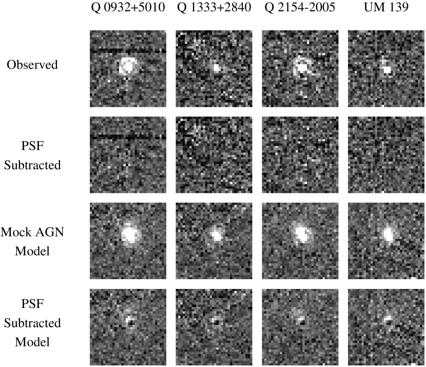
Figure 1: The observed narrow band image, the PSF-subtracted narrow-band image, a mock AGN model with the minimum amount of extended emission that we consider to be detectable, and the PSF-subtracted model for all objects observed with NICMOS camera 1. Each image is 1.5 $\times$ 1.5 arcsec.

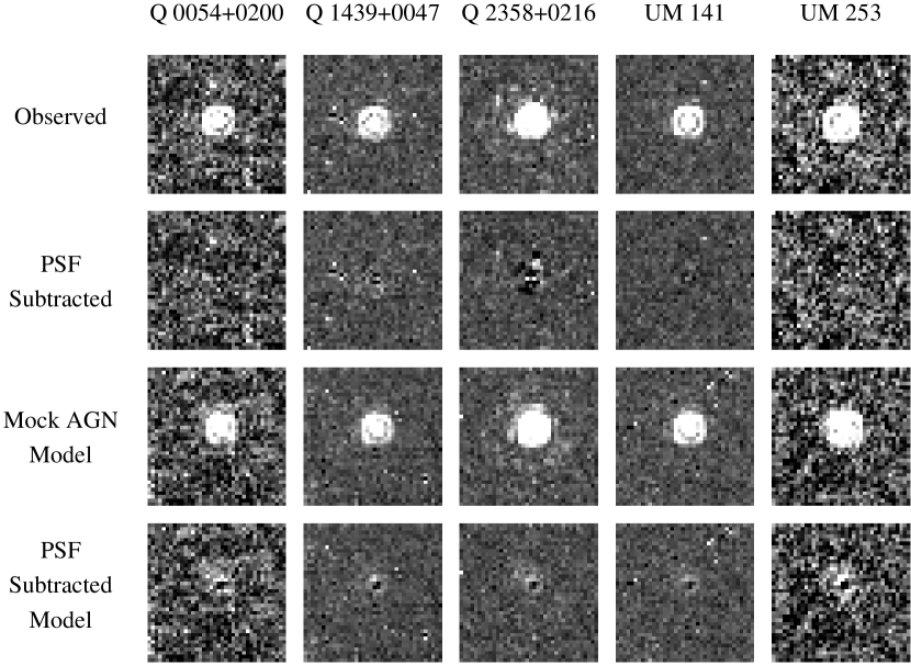
Figure 2: Same as Figure 1 for all objects observed with NICMOS camera 2. Each image is 3 $\times$ 3 arcsec.

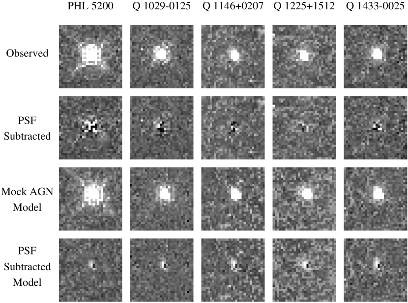
Figure 3: Same as Figure 1 and Figure 2 for all objects observed with NICMOS camera 3. Each image is 6 $\times$ 6 arcsec.

Although the observations permit us to measure the strength of the emission lines by this method, the primary purpose of the observations was to search for extended emission. None of the objects show any obvious extended emission from a simple visual inspection of the images (see Figures 1–3). To probe more sensitively for extended narrow-line emission, we need to remove the point-source contribution. We experimented with subtracting scaled broad-band images from the narrow-band images to create a continuum-subtracted image as is typically done for extended sources, but because the emission is (at least mostly) point-like, the resulting image is dominated by the residuals from the variation in PSFs between bands. Instead, we create PSF-subtracted narrow-band images, using the model PSFs generated individually for each object with Tiny Tim as discussed previously.

We use a simple iterative process to find the best-fit subtraction by minimizing the RMS deviation of the fit residuals. The position and normalization of the point source are varied as free parameters in the fitting process. The PSF subtractions worked quite well in general, particularly for cameras 1 and 2, although the camera 3 subtractions did leave some residuals. The PSF subtracted images are shown in the second row of Figure 1 for the NIC 1 images, Figure 2 for NIC 2, and Figure 3 for NIC 3. We measure the residual count rate after PSF subtraction in the same fixed aperture as before. These count rates are converted to flux, assuming the residual counts are due to a 400 ${\rm km\ s^{-1}}$ FWHM emission line at the expected wavelength for all lines. The results are shown in column 2 of Table 5. The quoted errors only include the individual pixel noise, so they do not include any uncertainty in the fits or the PSFs. Since we find residual fluxes both positive and negative well above this noise level, there are certainly additional sources of uncertainty. From inspection of the images, we conclude that all of the residual fluxes can be explained by either imperfect PSF subtractions or by variations in the background, probably associated with flatfield features not entirely removed by the pedestal correction.

As a final check on whether any extended emission is present in our images and to set upper limits on its absence, we create models to simulate the expected appearance of the extended emission in the image and the residuals from the PSF subtraction. To model the shape of the extended emission we use an appropriately scaled continuum-subtracted WFPC2 image in [O III] of NGC 1068 (Dressel et al., 1998). We assume the same size scaling for the extended emission of each model. The angular scale at the distance of NGC 1068 is 72 ${\rm pc\ arcsec^{-1}}$ (Bland-Hawthorn et al., 1997). Assuming $\Omega_{0}=1$ and $H_{0}=100\ h\ {\rm km\ s^{-1}\ Mpc^{-1}}$, the angular scale at $z=2$, approximately the mean redshift of our sample, is $4.1\ h^{-1}\ {\rm kpc\ arcsec^{-1}}$. For $h=0.75$, the angular scale is $5.5\ {\rm kpc\ arcsec^{-1}}$. To scale NGC 1068 up to the luminosity of a QSO, we assume that the NLR is optically thin and radiation bounded. Thus the physical size should scale roughly as the square root of the intensity of the ionizing radiation, which should scale roughly with bolometric luminosity. The bolometric luminosity of NGC 1068 is $L_{bol,NGC1068}\sim 4.2\times 10^{44}\ {\rm erg\ s^{-1}}$ (Pier et al., 1994), whereas a typical QSO in our sample has a bolometric luminosity of $L_{bol,QSO}\sim 2\times 10^{46}\ {\rm erg\ s^{-1}}$. We thus expect the NLR to be $\sim\sqrt{2\times 10^{46}/4.2\times 10^{44}}=6.9$ times larger in linear physical extent. Including the relative angular scales due to distance as described above, the overall size scaling to be applied to the NGC 1068 image to make it resemble a hypothetical BALQSO is $0.09$. We scale the NGC 1068 image by this amount and resample it to match the pixel size of the various NICMOS cameras. We normalize the flux for each model such that the total flux of the extended emission is some particular fraction of the aperture-corrected flux. We then convolve the model with the appropriate PSF and place it onto an empty section of the original image. A point source is added to the model, representing the remainder of the flux, such that the total flux of the point source plus extended component always equals the aperture-corrected value. This is then fit and subtracted using the same method as for the real data. We repeat this process for various fractions of extended emission relative to total flux in order to find at what minimum fraction the extended emission becomes detectable. We judge the extended emission to be detectable if some structure of several contiguous pixels above (or below) the background noise is visually apparent in the residuals. This process allows us to place an upper limit on the observed extended emission, albeit a subjective one.

The models with the minimum detectable fraction of extended emission are shown in row 3 of Figures 1–3. The PSF-subtracted models are shown in row 4 of the figures. Columns 3 and 4 of Table 5 list the narrow emission-line fluxes corresponding to the minimum detectable flux models and the residuals from the PSF subtractions of these models. These residuals were measured in the same fixed aperture as the other flux measurements and can thus be directly compared to the values from the real data in column 2. The residuals from the models are in most cases clearly larger than what was measured from the real data, consistent with our conclusion that we do not detect any extended flux. It is evident from comparing columns 3 and 4 of Table 5 that the fit requirement of minimizing the RMS deviation of the residuals results in a substantial amount of the extended flux being removed by the PSF subtraction, as much as $\sim 90$%.

Our tests using the models suggest that the presence of extended emission would result in excess flux in the first dark Airy ring as well as an over-subtracted core in the PSF-subtracted images, as can be seen in row 4 of Figures 1–3. The camera 1 and 2 data clearly show no such features in the PSF-subtracted images. For the only object observed with camera 1 or 2 with any significant residuals, Q 2358+0216, the residuals are along the first bright Airy ring and in the core. This is more indicative of an imperfect PSF subtraction than of extended emission. The camera 3 data are more difficult to judge. Although in principle camera 3 is most sensitive for our purpose due to the larger pixel scale and correspondingly lower read noise per unit angular area, the undersampling of the PSF makes the fits less certain and makes it difficult to determine if there is excess flux in the first dark Airy ring, which has a width of only $\sim 0.5$ pixels. Since the residuals from the camera 3 subtractions do not resemble closely those expected from the models, we conclude that the residuals are due to problems with the subtraction and are not indicative of extended emission.

4 DISCUSSION

To provide a context for the limits we have placed on the amount of extended emission, we use two separate methods to estimate the amount of extended emission we expected to observe. For the first estimate we assume that the equivalent widths of the narrow forbidden emission lines should be the same as for the composite spectrum of Francis et al. (1991). The equivalent widths for the composite are 15 Å for [O III] $\lambda$5007 and 1.9 Å for [O II] $\lambda$3727. To estimate narrow-line equivalent widths for the Balmer lines, we assume flux ratios of 10 for [O III] $\lambda$5007 / narrow H$\beta$ and 3 for narrow H$\alpha$ / narrow H$\beta$. These ratios are typical for Seyfert 2s and narrow-line radio galaxies (Koski, 1978). Assuming a continuum shape $F_{\nu}\propto\nu^{-0.3}$, we derive expected rest-frame equivalent widths of $\sim$7.5 Å for narrow H$\alpha$ and $\sim$1.5 Å for narrow H$\beta$. These equivalent widths are used to estimate narrow-line fluxes for each object, listed in column 5 of Table 5.

For the second estimate of the expected narrow-line flux we scale the observed flux of the emission lines in NGC 1068 (Koski, 1978) to the luminosity and distance of the QSOs in our sample. We assume that the flux of the lines scales linearly with bolometric luminosity. The bolometric luminosities of the QSOs are estimated as $\lambda F_{\lambda}$ as observed in the F160W filter. The luminosity distance for each QSO is calculated from the redshift assuming $\Omega=1$ and $h=0.75$. The line fluxes scaled from NGC 1068 are listed in column 7 of Table 5.

Columns 6 and 8 of Table 5 list the ratios of these fluxes to the minimum detectable flux in column 3 determined from the models. A ratio greater than unity would indicate that we would expect to have detected extended emission. However, only the NGC 1068 scaling for PHL 5200 exceeds unity. This object had the poorest PSF subtraction, so it is difficult to ascertain the existence of extended emission. Depending on the scaling, roughly half of the objects are above the 10% level, while some of the others are much smaller, well below our detection threshold. If the extended emission is at the level expected by these scaling arguments, it is not particularly surprising that we did not detect it. However, if the emission were only a few times stronger than what we expect based on these simple scaling arguments, then we should have been able to detect extended emission in some cases.

It is unfortunate that none of the six objects on the target list for our snapshot program matched for [O III] were observed, since the [O III] lines are expected to be the strongest emission lines in the NLR. For our scaling argument above, we assumed an [O III] $\lambda$5007 equivalent width of 15 Å. McIntosh et al. (1999) use infrared spectroscopy to study the rest-frame optical emission-line properties of a sample of QSOs with similar redshifts and luminosities to our sample. They find a mean equivalent width for [O III] $\lambda$5007 of 8.1 Å for seven BALQSOs and 11.6 Å for ten radio-quiet non-BALQSOs, but given the uncertainty and the small sample size the difference is not significant. These equivalent widths are somewhat lower than the mean of 23 Å for the 87 $z<0.5$ PG QSOs observed by Boroson & Green (1992). The low-redshift IR-selected QSO sample of Boroson & Meyers (1992) has even higher mean [O III] equivalent width of 46 Å for the 14 objects which were not low-ionization BALQSOs. Given these results, with even a conservative estimate of the strength of [O III], we would expect to observe [O III] line fluxes a factor of 3–5 greater than what we list in Table 5. We therefore might reasonably have expected to see extended emission in [O III] in 1–2 objects had they been observed.

The observed difference in H$\alpha$ equivalent widths between BALQSOs and non-BALQSOs merits further discussion. The mean rest-frame H$\alpha$ equivalent width for the BALQSOs is $390\pm 30$ Å, while the mean equivalent width for the non-BALQSOs is $200\pm 20$ Å, corresponding to a ratio $\langle{\rm EW}_{H\alpha}{\rm(BAL)}\rangle/\langle{\rm EW}_{H\alpha}{\rm(non-BAL)}\rangle=1.9\pm 0.2$. Even more striking than the ratio of the means is that the difference is systematic — all of the BALQSOs have larger H$\alpha$ equivalent widths than all of the non-BALQSOs. A two-sample K-S test yields that the BALQSO and non-BALQSO data were drawn from separate populations with 99.3% confidence, although given that the sample groups are small and certainly incomplete, one should approach this number with caution. However, the data are suggestive of a possible real systematic difference between the two groups.

We have considered the possibility that the difference in equivalent widths could be due to some systematic difference in the observations. The observations were performed over roughly the same time period and with the same filters and cameras for both groups. However, there is a systematic difference in the location of the H$\alpha$ line in the filters. For all of the non-BALQSOs, the expected location of the peak of the broad H$\alpha$ emission line lies near the center of the filter bandpass, while for the BALQSOs the peak of the line lies near the edge of the bandpass, resulting in larger corrections for flux outside the bandpass. This can be seen by comparing the values in column 9 of Table 3 for the BALQSOs and non-BALQSOs. For three of the BALQSOs the emission line center is longward of the center of the filter, while for the other two it is shortward. The systematic difference in the location of the lines in the filters renders the effect of making the relative H$\alpha$ equivalent widths of the BALQSOs and non-BALQSOs sensitive to the assumed profile shape. We find that if we assume a broader line profile, the disparity between the two groups diminishes but does not disappear. If we use the conversion factors from column 6 of Table 3, calculated assuming a Gaussian profile with a FWHM of 5000 ${\rm km\ s^{-1}}$, the ratio of equivalent widths becomes $\langle{\rm EW}_{H\alpha}{\rm(BAL)}\rangle/\langle{\rm EW}_{H\alpha}{\rm(non-BAL)}\rangle=1.6\pm 0.2$.

There are several possible systematic differences between BALQSOs and non-BALQSOs that could explain our observations. The most straightforward explanation is that there is simply more H$\alpha$ flux in BALQSOs than non-BALQSOs. Another possibility is that the H$\alpha$ lines could have the same flux on average but be systematically much broader in the non-BALQSOs. Either one of these would be extremely surprising, however, since broad emission lines in the UV exhibit no large systematic differences (Weymann et al., 1991). Also, McIntosh et al. (1999) do not find large differences in H$\beta$ emission between BALQSOs and non-BALQSOs. An even more intriguing possibility is that the continua are different in BALQSOs and non-BALQSOs, since in all cases we have estimated the continuum in the narrow-band filter from shorter wavelength F160W images. If the continuum shape were redder than we have assumed in BALQSOs, we would underestimate the continuum in the narrow-band images of the BALQSOs, resulting in larger fluxes and equivalent widths. The implied continuum shape in the rest-frame optical for BALQSOs that would account for the systematically larger H$\alpha$ equivalent widths has an effective power-law index $\alpha_{\nu}=-1.9$, compared to the typical $\alpha_{\nu}=-0.3$ that we assumed. This amount of reddening is comparable with that observed in low-ionization BALQSOs (Weymann et al., 1991) and attributed to intrinsic dust extinction (Sprayberry & Foltz, 1992). In fact, two of the BALQSOs in our sample, PHL 5200 and Q 2358+0216, are low-ionization BALQSOs, so it is not surprising that we derive larger H$\alpha$ equivalent widths for these objects. However, the fact that the other three BALQSOs follow the same trend is interesting, since there is generally little evidence from rest-frame UV spectra for intrinsic dust extinction in high-ionization BALQSOs (Weymann et al., 1991). To investigate whether there is an overall reddening of the continuum in our sample, we used our fluxes in the F160W band for each object along with the fluxes at $\sim 2100$ Å in the rest frame calculated from optical spectra by Weymann et al. (1991) to derive $(R-H)$ color indices. For the two QSOs in our sample not in Weymann et al. (1991), Q 0054+0200 and Q 2358+0216, we estimate the optical flux from the $B_{J}$ magnitudes in the LBQS catalog (Hewett, Foltz, & Chaffee, 1995). Of the objects observed in H$\alpha$, we find that both the BALQSO and non-BALQSO groups have $\langle(R-H)\rangle=1.95$ with $\sigma\sim 0.8\ {\rm mag}$, suggesting that there is no significant systematic difference in the continuum properties in our sample in the rest-frame 2100–5500 Å spectral region. Near-infrared (rest-frame optical) spectroscopy of BALQSOs is necessary to resolve this issue.

5 SUMMARY

We have obtained HST NICMOS snapshot images of ten BALQSOs and four non-BALQSOs to search for extended narrow-line emission. Each object was imaged in both the F160W filter and a narrow-band filter corresponding to H$\alpha$, H$\beta$, or [O II]. Using aperture photometry, we derive estimates of the emission-line fluxes and equivalent widths. To look for extended emission, we use model PSFs to generate PSF-subtracted narrow-band images. We measure the residual flux in these images and compared them to PSF-subtracted images of simulated data. Our most important results are:

1. We do not detect extended emission in any of the images. Some of the images have PSF-subtraction residuals, but based on comparisons with simulated data we conclude that the residuals are the result of imperfect PSF subtraction and are not evidence for extended emission.

2. We find that for the nine objects we observed in H$\alpha$, we derive systematically larger equivalent widths for the five BALQSOs than for the four non-BALQSOs, by a factor of 1.9 on average. Given the small sample size, it is not certain whether this is a real effect or just a statistical aberration. If it is real, it could be evidence either for an intrinsic difference between BALQSOs and non-BALQSOs in H$\alpha$ emission, or for systematically redder rest-frame optical continua in BALQSOs, an effect which has been observed in low-ionization BALQSOs. If either of these differences were real, it would stand in stark contrast to studies of rest-frame UV spectra which find little difference between the continuum and emission-line properties of high-ionization BALQSOs and radio-quiet non-BALQSOs.

Table 1: Observations

					Broad-Band	Narrow-Band
Object	Redshift	BAL?	Date	Camera	Filter	Filter
PHL 5200	1.981	Y	1998 June 16	3	F160W	F196N
Q 0021-0213	2.348	Y	1998 October 10	1	F160W	F164N
Q 0054+0200	1.872	Y	1998 August 3	2	F160W	F187N
Q 0932+5010	1.914	Y	1998 September 13	1	F160W	F108N
Q 1029-0125	2.029	Y	1998 June 20	3	F160W	F200N
Q 1146+0207	2.054	N	1998 March 15	3	F160W	F200N
Q 1225+1512	1.990	N	1998 June 14	3	F160W	F196N
Q 1333+2840	1.908	Y	1998 November 10	1	F160W	F108N
Q 1433-0025	2.042	N	1998 May 8	3	F160W	F200N
Q 1439+0047	1.857	N	1998 July 10	2	F160W	F187N
Q 2154-2005	2.035	Y	1998 October 26	1	F160W	F113N
Q 2358+0216	1.872	Y	1998 August 16	2	F160W	F187N
UM 139	2.029	Y	1998 October 18	1	F160W	F113N
UM 141	2.909	Y	1998 September 27	2	F160W	F190N
UM 253	2.253	Y	1998 October 31	2	F160W	F212N

Table 2: Aperture Photometry

	Broad-Band Count Rates		Narrow-Band Count Rates
Object	Measured	Corrected	Measured	Corrected	$AB_{F160W}$
PHL 5200	$249.7\pm 0.8$	$258.4\pm 0.8$	$62.9\pm 0.1$	$71.8\pm 0.1$	$16.821\pm 0.003$
Q 0021-0213	$105.1\pm 3.1$	$115.8\pm 3.4$	$5.1\pm 0.3$	$5.6\pm 0.4$	$17.793\pm 0.032$
Q 0054+0200	$75.9\pm 1.4$	$84.4\pm 1.5$	$13.2\pm 0.2$	$14.6\pm 0.2$	$18.294\pm 0.019$
Q 0932+5010	$273.8\pm 2.5$	$301.6\pm 2.7$	$4.1\pm 0.2$	$4.5\pm 0.2$	$16.754\pm 0.010$
Q 1029-0125	$113.0\pm 0.7$	$116.9\pm 0.7$	$22.1\pm 0.1$	$25.3\pm 0.1$	$17.682\pm 0.006$
Q 1146+0207	$123.3\pm 0.7$	$127.6\pm 0.7$	$14.8\pm 0.1$	$17.0\pm 0.1$	$17.505\pm 0.006$
Q 1225+1512	$74.4\pm 1.2$	$77.0\pm 1.2$	$16.4\pm 0.1$	$18.7\pm 0.1$	$18.136\pm 0.017$
Q 1333+2840	$96.7\pm 3.5$	$106.5\pm 3.8$	$1.5\pm 0.3$	$1.6\pm 0.3$	$17.884\pm 0.039$
Q 1433-0025	$64.8\pm 0.6$	$67.1\pm 0.6$	$11.0\pm 0.1$	$12.1\pm 0.1$	$18.204\pm 0.010$
Q 1439+0047	$68.1\pm 1.5$	$75.7\pm 1.7$	$10.7\pm 0.2$	$12.1\pm 0.2$	$18.413\pm 0.024$
Q 2154-2005	$155.2\pm 3.2$	$171.0\pm 3.5$	$3.9\pm 0.3$	$4.2\pm 0.3$	$17.370\pm 0.022$
Q 2358+0216	$214.7\pm 1.4$	$238.7\pm 1.5$	$35.2\pm 0.2$	$39.0\pm 0.2$	$17.165\pm 0.007$
UM 139	$78.5\pm 3.0$	$86.5\pm 3.3$	$1.3\pm 0.3$	$1.4\pm 0.3$	$18.110\pm 0.041$
UM 141	$207.4\pm 1.4$	$230.6\pm 1.5$	$13.8\pm 0.1$	$15.3\pm 0.2$	$17.203\pm 0.007$
UM 253	$97.4\pm 1.4$	$108.3\pm 1.5$	$21.6\pm 0.2$	$23.8\pm 0.2$	$18.023\pm 0.015$

Table 3: Emission Line Flux Conversion Factors

	Emission	Redshifted	Filter
Object	Line	$\lambda_{peak}$(Å)	$\lambda_{eff}$(Å)	A	B	B/A	C	A/C
(1)	(2)	(3)	(4)	(5)	(6)	(7)	(8)	(9)
PHL 5200	H$\alpha$	19569	19639	1.986	2.430	1.22	1.017	1.95
Q 0054+0200	H$\alpha$	18854	18740	2.976	3.259	1.10	1.805	1.65
Q 0932+5010	[O II]	10865	10816	13.40	$\cdots$	$\cdots$	7.592	1.77
Q 1029-0125	H$\alpha$	19884	19975	2.147	2.480	1.10	1.584	1.36
Q 1146+0207	H$\alpha$	20048	19975	1.823	2.354	1.29	1.584	1.15
Q 1225+1512	H$\alpha$	19628	19639	1.621	2.193	1.35	1.017	1.59
Q 1333+2840	[O II]	10842	10816	7.665	$\cdots$	$\cdots$	7.592	1.01
Q 1433-0025	H$\alpha$	19970	19975	1.589	2.111	1.33	1.584	1.00
Q 1439+0047	H$\alpha$	18755	18740	1.807	2.438	1.35	1.805	1.00
Q 2154-2005	[O II]	11316	11298	5.880	$\cdots$	$\cdots$	6.110	0.96
Q 2358+0216	H$\alpha$	18854	18740	2.976	3.259	1.10	1.805	1.65
UM 139	[O II]	11294	11298	6.279	$\cdots$	$\cdots$	6.110	1.03
UM 141	H$\beta$	19008	19004	1.760	2.420	1.38	1.759	1.00
UM 253	H$\alpha$	21355	21213	2.722	2.757	1.01	1.391	1.96

Table 4: Emission Line Data

		Narrow-Band Count Rates			Equivalent Width (Å)
		Scaled	Net	Integrated
Object	Line	Continuum	Emission Line	Line Flux	Observed	Rest Frame
PHL 5200	H$\alpha$	$15.2^{+1.8}_{-2.0}$	$56.6^{+2.0}_{-1.8}$	$113^{+5}_{-5}$	$1300^{+220}_{-200}$	$438^{+74}_{-65}$
Q 0054+0200	H$\alpha$	$4.42^{+0.42}_{-0.47}$	$10.19^{+0.50}_{-0.45}$	$30.3^{+1.7}_{-1.6}$	$1050^{+160}_{-140}$	$364^{+56}_{-50}$
Q 0932+5010	[O II]	$4.3^{+0.9}_{-1.2}$	$0.2^{+1.2}_{-0.9}$	$3^{+16}_{-13}$	$8^{+54}_{-43}$	$3^{+18}_{-15}$
Q 1029-0125	H$\alpha$	$7.2^{+0.9}_{-1.0}$	$18.1^{+1.1}_{-0.9}$	$38.9^{+2.5}_{-2.2}$	$1030^{+210}_{-180}$	$339^{+69}_{-60}$
Q 1146+0207	H$\alpha$	$7.8^{+1.0}_{-1.1}$	$9.2^{+1.1}_{-1.0}$	$16.7^{+2.2}_{-1.9}$	$400^{+110}_{-90}$	$133^{+36}_{-31}$
Q 1225+1512	H$\alpha$	$4.54^{+0.54}_{-0.61}$	$14.14^{+0.62}_{-0.54}$	$22.9^{+1.2}_{-1.1}$	$890^{+160}_{-140}$	$299^{+53}_{-47}$
Q 1333+2840	[O II]	$1.53^{+0.33}_{-0.41}$	$0.10^{+0.50}_{-0.44}$	$0.8^{+3.9}_{-3.3}$	$7^{+38}_{-32}$	$3^{+13}_{-11}$
Q 1433-0025	H$\alpha$	$4.10^{+0.52}_{-0.60}$	$7.96^{+0.60}_{-0.52}$	$12.7^{+1.0}_{-0.9}$	$580^{+130}_{-110}$	$191^{+42}_{-37}$
Q 1439+0047	H$\alpha$	$3.96^{+0.38}_{-0.42}$	$7.87^{+0.45}_{-0.42}$	$14.2^{+0.9}_{-0.9}$	$550^{+90}_{-80}$	$191^{+31}_{-28}$
Q 2154-2005	[O II]	$3.03^{+0.58}_{-0.72}$	$1.19^{+0.77}_{-0.65}$	$7.0^{+4.6}_{-3.8}$	$44^{+38}_{-32}$	$14^{+13}_{-10}$
Q 2358+0216	H$\alpha$	$12.5^{+1.2}_{-1.3}$	$26.5^{+1.3}_{-1.2}$	$79^{+5}_{-4}$	$960^{+150}_{-130}$	$335^{+52}_{-46}$
UM 139	[O II]	$1.53^{+0.30}_{-0.37}$	$-0.17^{+0.46}_{-0.40}$	$-1.1^{+2.9}_{-2.5}$	$-14^{+33}_{-29}$	$-4^{+11}_{-10}$
UM 141	H$\beta$	$11.9^{+1.2}_{-1.3}$	$3.5^{+1.4}_{-1.2}$	$6.1^{+2.4}_{-2.2}$	$79^{+40}_{-36}$	$20^{+11}_{-9}$
UM 253	H$\alpha$	$6.7^{+1.1}_{-1.3}$	$17.2^{+1.3}_{-1.2}$	$46.8^{+3.7}_{-3.2}$	$1550^{+410}_{-340}$	$480^{+120}_{-100}$

Table 5: PSF Subtraction Residuals

				Composite QSO Scaling		NGC 1068 Scaling
	Residual	Minimum	Model	Expected		Expected
Object	Flux	Detectable Flux	Residual Flux	Line Flux	Ratio	Line Flux	Ratio
PHL 5200	$2.8\pm 0.1$	4.9	0.4	1.9	0.39	6.0	1.21
Q 0054+0200	$-0.5\pm 1.1$	33	7.7	0.6	0.02	1.5	0.05
Q 0932+5010	$-4.8\pm 2.7$	30	19.6	1.7	0.06	1.1	0.04
Q 1029-0125	$0.1\pm 0.1$	6	0.6	0.9	0.16	2.7	0.49
Q 1146+0207	$-0.1\pm 0.1$	10	1.1	0.9	0.09	3.2	0.30
Q 1225+1512	$0.5\pm 0.1$	13	1.3	0.6	0.05	1.8	0.14
Q 1333+2840	$1.8\pm 2.3$	16	5.1	0.6	0.04	0.4	0.02
Q 1433-0025	$0.5\pm 0.1$	7	0.6	0.5	0.07	1.7	0.23
Q 1439+0047	$0.9\pm 0.3$	5	0.9	0.6	0.12	1.4	0.30
Q 2154-2005	$4.5\pm 1.8$	15	6.2	0.9	0.06	0.6	0.04
Q 2358+0216	$-2.2\pm 1.1$	22	6.4	1.8	0.08	4.4	0.20
UM 139	$-1.6\pm 1.9$	16	6.2	0.5	0.03	0.3	0.02
UM 141	$-0.4\pm 0.1$	4	0.7	0.5	0.12	0.9	0.25
UM 253	$-7.3\pm 1.9$	114	29.2	0.7	0.01	2.0	0.02

References

- Antonucci (1993) Antonucci, R. 1993, ARA&A, 31, 473
- Bland-Hawthorn et al. (1997) Bland-Hawthorn, J., Gallimore, J. F., Tacconi, L. J., Brinks, E., Baum, S. A., Antonucci, R. R. J., & Cecil, G. N. 1997, Ap&SS, 248, 9
- Boroson & Green (1992) Boroson, T. A., & Green, R. F. 1992, ApJS, 80, 109
- Boroson & Meyers (1992) Boroson, T. A., & Meyers, K. A. 1992, ApJ, 397, 442
- Boroson & Oke (1984) Boroson, T. A., & Oke, J. B. 1984, ApJ, 281, 535
- Boroson, Persson, & Oke (1985) Boroson, T. A., Persson, S. E., & Oke, J. B. 1985, ApJ, 293, 120
- Cohen et al. (1995) Cohen, M. H., Ogle, P. M., Tran, H. D., Vermeulen, R. C., Miller, J. S., Goodrich, R. W., & Martel A. R. 1995, ApJ, 448, L77
- Dressel et al. (1998) Dressel, L. L., Tsvetanov, Z. I., Kriss, G. A., & Ford, H. C. 1998, Ap&SS, 248, 85
- Durret et al. (1994) Durret, F., Pécontal, E., Petitjean, P., & Bergeron, J. 1994, A&A, 291, 392
- Evans et al. (1993) Evans, I. N., Tsvetanov, Z., Kriss, G. A., Ford, H. C., Caganoff, S., & Koratkar, A. P. 1993, ApJ, 417, 82
- Foltz et al. (1990) Foltz, C. B., Chaffee, F. H., Hewett, P. C., Weymann, R. J., & Morris, S. L. 1990, BAAS, 22, 806
- Francis et al. (1991) Francis, P. J., Hewitt, P. C., Foltz, C. B., Chaffee, F. H., Weymann, R. J., & Morris, S. L. 1991, ApJ, 373, 465
- Goodrich (1997) Goodrich, R. W. 1997, ApJ, 474, 606
- Goodrich & Miller (1995) Goodrich, R. W., & Miller, J. S. 1995, ApJ, 448, L73
- Hamann, Korista, & Morris (1993) Hamann, F., Korista, K. T., & Morris, S. L. 1993, ApJ, 415, 541
- Hes, Barthel, & Fosbury (1996) Hes, R., Barthel, P. D., & Fosbury, R. A. E. 1996, A&A, 313, 423
- Hewett, Foltz, & Chaffee (1995) Hewett, P. C., Foltz, C. B., & Chaffee, F. H. 1995, AJ, 109, 1498
- Jackson & Browne (1991) Jackson, N., & Browne, I. W. A. 1991, MNRAS, 250, 414
- Koski (1978) Koski, A. T. 1978, ApJ, 223, 56
- Kriss et al. (1995) Kriss, G. A., Davidsen, A. F., Zheng, W., Kruk, J. W., & Espey, B. R. 1995, ApJ, 454, L7
- Kriss et al. (1996) Kriss, G. A., Espey, B. R., Krolik, J. H., Tsvetanov, Z., Zheng, W., & Davidsen, A. F. 1996, ApJ, 467, 622
- Kriss et al. (1992) Kriss, G. A., et al. 1992, ApJ, 392, 485
- Krist (1993) Krist, J. 1993, in ASP Conf. Proc. 52, Astronomical Data Analysis Software and Systems II, ed. R. J. Hanisch, R. J. V. Brissenden, & J. Barnes (San Francisco: ASP), 536
- Krolik & Voit (1998) Krolik, J. H., & Voit, G. M. 1998, ApJ, 497, L5
- Malkan, Gorjian, & Tam (1998) Malkan, M. A., Gorjian, V., & Tam, R. 1998, ApJS, 117, 25
- McIntosh et al. (1999) McIntosh, D. H., Rieke, M. J., Rix, H.-W., Foltz, C. B, & Weymann, R. J. 1999, ApJ, 514, 40
- Miyaji, Wilson, & Pérez-Fournon (1992) Miyaji, T., Wilson, A. S., & Pérez-Fournon, I. 1992, ApJ, 385, 137
- Mulchaey, Wilson, & Tsvetanov (1996) Mulchaey, J. S., Wilson, A. S., & Tsvetanov, Z. 1996, ApJ, 467, 197
- Penston (1981) Penston, M. V., et al. 1981, MNRAS, 196, 857
- Pier et al. (1994) Pier, E. A., Antonucci, R., Hurt, T., Kriss, G., & Krolik, J. 1994, ApJ, 428, 124
- Schmitt & Kinney (1996) Schmitt, H. R. & Kinney, A. L. 1996, ApJ, 463, 498
- Skinner & Bergeron (1997) Skinner, C. J., & Bergeron, L. 1997, NICMOS Instrument Science Rep. (NICMOS-97-026; Baltimore: STScI)
- Sprayberry & Foltz (1992) Sprayberry, D., & Foltz, C. B. 1992, ApJ, 390, 39
- Stockton & MacKenty (1987) Stockton, A., & MacKenty, J. W. 1987, ApJ, 316, 584
- Ulrich & Boisson (1983) Ulrich, M.-H., & Boisson, C. 1983, ApJ, 267, 515
- Weymann et al. (1991) Weymann, R. J., Morris, S. L., Foltz, C. B., & Hewett, P. C. 1991, ApJ, 373, 23