Efficiencies of Low-Mass Star and Star Cluster Formation

Abstract

Using a quantitative model for bipolar outflows driven by hydromagnetic protostellar winds, we calculate the efficiency of star formation assuming that available gas is either converted into stars or ejected in outflows. We estimate the efficiency of a single star formation event in a protostellar core, finding $25\%-70\%$ for cores with various possible degrees of flattening. The core mass function and the stellar initial mass function have similar slopes, because the efficiency is not sensitive to its parameters. We then consider the disruption of gas from a dense molecular clump in which a cluster of young stars is being born. In both cases, we present analytical formulae for the efficiencies that compare favorably against observations and, for clusters, against numerical simulations. We predict efficiencies in the range $30\%-50\%$ for the regions that form clusters of low-mass stars. In our model, star formation and gas dispersal happen concurrently. We neglect the destructive effects of massive stars: our results are therefore upper limits to the efficiency in regions more massive than about $3000~{}{\rm M}_{\mathord{\odot}}$.

1. Introduction

Star formation in molecular clouds is a slow and seemingly inefficient process. Clouds are transformed into stars far more slowly than gravity would allow (Zuckerman & Palmer 1974); only the deepest regions of clouds participate in star formation (McKee 1989; Li, Evans, & Lada 1997); star-forming regions are disrupted before star formation is complete (Lada, Margulis, & Dearborn 1984); and individual protostellar cores may also shed mass on their way to stardom (Benson & Myers 1989; Ladd, Fuller, & Deane 1998). A growing appreciation for the violence and ubiquity of protostellar outflows has led many authors to suggest that outflows provide the mechanism to regulate star formation and to dissipate star-forming gas, especially in regions that lack massive stars. Protostellar outflows have been implicated in the support of molecular clouds and cluster-forming clumps against gravity (Norman & Silk 1980; Lada & Gautier 1982; McKee 1989; Bertoldi & McKee 1996) and in the removal of gas from star-forming regions (Levreault 1984; Langer, Frerking, & Wilson 1986; Goldsmith, Langer, & Wilson 1986; Umemoto, Hirano, Kameya, Fukui, Kuno, & Takakubo 1991; Bally & Duvert 1994; Bally, Reipurth, Lada, & Billawala 1999) or from protostellar cores (Myers, Heyer, Snell, & Goldsmith 1988; Nakano, Hasegawa, & Norman 1995; Velusamy & Langer 1998; Ladd, Fuller, & Deane 1998). In this paper, we shall construct quantitative models to determine the destructive effects of outflows on the molecular cores that make individual stars, and on the larger molecular clumps that make star clusters. Disruption by outflows limits the efficiency of low-mass star formation; it relates the mass function of cores to the stellar initial mass function; and it determines whether a young stellar system will remain bound.

1.1. Disruption of Protostellar Cores

The most direct progenitors of stars are dense cores within star-forming regions. The distribution of initial stellar masses is therefore controlled by two factors: the distribution of core masses, and the fraction of a given core that can successfully become a star (Nakano, Hasegawa, & Norman 1995). Recent observations of the core mass distribution by Motte et al. (1998) indicate a similarity to the initial mass function (IMF).

Several authors have made theoretical predictions for the manner in which a protostar’s wind truncates its own accretion, limiting the core mass that becomes stellar. Silk (1995) matched the Kelvin-Helmholtz luminosity of the protostar with the accretion luminosity of its disk (in the model of Terebey et al. 1984) to find the point at which disk accretion stops. Similarly, Adams & Fatuzzo (1996) matched the ram pressure of material falling directly onto the stellar surface (in the same infall model) with the wind ram pressure; although it is more physical to consider ram pressures than luminosities, this theory does not explain what stops disk accretion. Nakano et al. (1995) took a distinctly different approach: recognizing that material falling onto the disk might circumvent the outflow, they instead considered the disruption of the larger-scale density distribution of the accreting core. Idealizing the core material as static, they argued that accretion would stop once a momentum-conserving wind bubble (or a stellar HII region) had traversed its radius. For fiducial values of the parameters, they find quite low efficiencies, of order a few percent.

All of these models have considered only spherical protostellar winds, and they have generally not treated anisotropies in the protostellar core material (besides centrifugal deflection of the infall). However, the winds from young stars are collimated into jets on a short length scale, and the core is likely to be somewhat flattened because of support from poloidal magnetic fields. Li & Shu (1996) incorporated these very elements into a model for the early phase of a molecular outflow, during which it propagates into its own protostellar core. However, Li & Shu did not consider the implications of this model for the efficiency protostellar accretion.

In §5 we shall construct a model for the disruption of an accreting, somewhat flattened protostellar core. Assuming that the wind intensity is directly proportional to the accretion rate, as in the X-wind model (Shu et al. 1994), and in some disk-wind models (Pelletier & Pudritz 1992), we identify the angle from the axis within which core material is ejected and outside of which it is accreted. As in the model of Nakano et al. (1995), and also as argued by Mouschovias (1991), protostellar accretion is terminated by the finite size of the protostellar core; however, the efficiency with which the star forms is a function both of the flattening of the core, and the ratio of its sound speed to the characteristic wind velocity. We compare the results of this calculation to observations of core disruption and constraints on the efficiency of core collapse in §5.4.

1.2. Disruption of Cluster-Forming Clumps

A protostellar wind can have destructive effects on regions considerably larger and more massive than its own protostellar core, repercussions that have implications for the fates of young stellar clusters.

Stars are born in groups, deeply embedded within dense clumps of molecular gas. The fate of a nascent stellar system – whether to become an expanding association or to remain a bound open cluster – is determined by how rapidly and effectively it breaks free of the gas from which it was created. This process is primarily controlled by two parameters: the efficiency of star formation, defined as the fraction of gas converted into stars, and the time scale on which the remaining gas is disrupted. If the gas removal is rapid relative to the free-fall time $t_{\rm ff}$, then more than half the mass must be in stars for the cluster to remain bound (Hills 1980). On the other hand, sufficiently slow mass loss allows a virialized stellar system to expand adiabatically and to remain bound. Lada et al. (1984) studied intermediate cases, in which they found that part of the cluster was likely to escape even if a fraction remained bound.

Empirically, roughly only a tenth of all stars remain bound in clusters (Miller & Scalo 1978). The interactions between stars and gas must produce this statistic, yet the underlying mechanism by which gas is dispersed remains largely mysterious. Most stars are born in large OB associations (e.g., McKee & Williams 1997), and the violent effects of the massive stars in these associations have the potential to disrupt the star-forming gas; however, this can only be in addition to the disruptive effects of the low-mass stars themselves.

We shall take the embedded clusters in L1640 as prototypical examples of groups of low-mass stars in the process of formation. As described by Lada et al. (1991) and Lada (1992), these clusters have several hundred stars apiece; they are coincident with the densest and most massive molecular clumps in the region. Stars currently constitute about $40\%$ of the total mass in the two largest clumps, but the others show a much smaller stellar fraction. Moreover, star formation is restricted to these regions (Li et al. 1997). This observation is consistent with the theory of McKee (1989) that stars form only in regions of high extinction and therefore low ionization, so that ambipolar diffusion can lead to the creation of protostellar cores. It lends credence to the idea that the gas and stars can be treated as a finite, self-gravitating system of a definite mass and radius (see also Mathieu 1983), a notion we shall use in our analysis.

In §6, we calculate the amount of gas removed from a clump by the bipolar molecular outflows driven by the stars themselves. There is ample evidence for the importance of gas removal by outflows from star-forming regions: note, for instance, the disruptions of PV Cephei (Levreault 1984), B335 (Langer et al. 1986), Lynds 1221 (Umemoto et al. 1991), HH83 (Bally & Duvert 1994), and Circinus (Bally et al. 1999), and the eruptions of the IRS3 outflow from Barnard 5 (Goldsmith et al. 1986) and of the HH300 outflow from Taurus (Arce & Goodman 2000). Indeed, any example of protostellar jets and Herbig-Haro objects outside the source’s parent cloud implies that potentially star-forming gas has been ejected. Individual protostellar winds are thus remarkable in their ability to affect pre-stellar cores (on $\sim 0.05~{}{\rm pc}$ scales), cluster forming clumps ($\sim 0.4-1~{}{\rm pc}$) and giant molecular clouds ($\sim 10-100~{}{\rm pc}$), as evinced by the existence of parsec-scale flows (Reipurth et al. 1997).

We shall gauge mass ejection using the model for protostellar outflows presented in a previous paper (Matzner & McKee 1999). This model generalizes the force distribution predicted in the X-wind model (Shu et al. 1995) to a much wider class of winds. The interaction of the protostellar wind with the ambient medium occurs in a thin, radiative shell that conserves the wind momentum and ambient mass in each direction. In §4 we use this model to calculate the criterion for the outflow shell to be ejected in a particular direction. The mass loss from such outflows is estimated analytically in §6. The principal idealization in our treatment is that each star forms at the exact center of the clump distribution. Therefore, we present in §6.1 a numerical evaluation of the gas lost from a model clump, in which star formation is distributed according to the local ambipolar diffusion rate (McKee 1989). In the Appendix, we evaluate the detailed effect of gravity on the motion of an outflow shell.

Our analysis suggests that a significant amount of mass can be lost during the process of star formation itself. Indeed, the rate at which mass is lost due to outflows is several times the rate at which gas is converted into stars. However, we do not consider the disruptive effects of massive stars, which might cause gas to be removed more rapidly. Our results are therefore only rough upper limits for the star formation efficiency in clumps more massive than about $3000~{}{\rm M}_{\mathord{\odot}}$, in which O stars will form.

Unlike most previous work (e.g., Nakano et al. 1995), we divide the calculation of star formation efficiency into two parts: the disruption of a star’s own protostellar core, and the disruption of a clump in which an aggregate of young stars is forming. Different assumptions are appropriate for the two cases. For a core, the rates of accretion and outflow are directly proportional; the axes along which the core is flattened and the wind is collimated are likely to be aligned; the wind duration exceeds the free-fall time; and the density distribution declines with radius approximately as $r^{-2}$. For the disruption of a cluster-forming clump, opposite assumptions apply: for instance, winds are impulsive and not likely to correlate in direction with the clump’s structure.

1.3. Estimate of the Star Formation Efficiency

Before getting into the details of the calculation, it is worthwhile to make a simple estimate of the outcome. The star formation efficiency for the formation of a single star is

$$\varepsilon=\frac{m_{\star}}{m_{\star}+M_{\rm ej}},$$ (1)

where $M_{\rm ej}$ is the mass ejected from the protostellar core or star forming clump due to the formation of a single star of mass $m_{\star}$ (see §2 below). The total momentum in the wind is $p_{w}=m_{w}v_{w}$. We assume that the mass of the wind is a fraction $f_{w}$ of the stellar mass, so that $m_{w}=f_{w}m_{\star}$ and $p_{w}=f_{w}m_{\star}v_{w}$. This momentum is transferred to the cloud by radiative shocks; as described above, such a model is in good agreement with observation (Matzner & McKee 1999). In order for the shocked gas to escape from the cloud, it must be moving at least at the escape velocity, $v_{\rm esc}$. Since the shocked gas has momentum $p_{w}$, the ejected mass is a maximum if all the gas has this minimum velocity, $M_{\rm ej}\sim p_{w}/v_{\rm esc}.$ Assuming for the moment that this mass is large compared to the mass of the star that forms, as in the model of Nakano et al. (1995), we estimate the star formation efficiency as

$$\varepsilon\simeq\frac{m_{\star}}{M_{\rm ej}}\simeq\frac{m_{\star}c_{g}v_{\rm esc}}{p_{w}}\simeq\frac{c_{g}v_{\rm esc}}{f_{w}v_{w}},$$ (2)

where the factor $c_{g}\geq 1$ allows for the decrease in the momentum of the shocked shell due to the self-gravity of the core or clump.

This argument can be refined by taking into account the central fact about protostellar winds, that they are collimated. As originally shown by Shu et al. (1995) and demonstrated more generally by Matzner & McKee (1999), the wind momentum falls off approximately as $1/(\sin\theta)^{2}$ for $\theta>\theta_{0}$, where $\theta$ is measured from the axis of the wind and $\theta_{0}\sim 10^{-2}$ is discussed in §3 below. The momentum inside $\theta$ thus scales as $\ln(1/\theta)$: equal amounts of momentum are contained in each octave of angle. Since the area covered by the wind, and therefore the mass swept up, is dominated by the largest angle, it follows that most of the mass that escapes will indeed have the minimum possible velocity ($\sim v_{\rm esc}$), as assumed above. Furthermore, since the momentum is spread out logarithmically, only a fraction $\sim 1/\ln(1/\theta_{0})$ of the total momentum is available to eject matter at $v\sim v_{\rm esc}$. As a result, the star formation efficiency estimated above should be multiplied by this quantity. The calculations below show that this fraction is more precisely given by $\sim 1/\ln(2/\theta_{0})$. Defining the efficiency factor $X$ by

$$X\equiv\frac{c_{g}v_{\rm esc}\ln(2/\theta_{0})}{f_{w}v_{w}},$$ (3)

we conclude that for small values of $X$, the star formation efficiency $\varepsilon\sim X$; at large values of $X$, we expect $\varepsilon$ to approach its maximum possible value, unity. These expectations are borne out by the results presented below. Observe that the collimation of the wind reduces the mass that can be ejected by a factor $\sim 1/\ln(2/\theta_{0})\sim 0.2$ and increases the star formation efficiency by the same factor. As a result, our estimates of $\varepsilon$ are significantly higher than those of Nakano et al. (1995) and are in much closer agreement with observation.

2. Instantaneous, Observational and Total Star Formation Efficiencies

We begin by discussing the various possible definitions of the star formation efficiency. For the collapse of a protostellar core to form a single star (or a binary) there is only one efficiency that can be defined, namely the ratio of the star’s (or binary’s) mass to that of its parent core:

$$\varepsilon=\varepsilon_{\rm core}\equiv\frac{m_{\star}}{M_{\rm core}}.$$ (4)

This definition is consistent with that in equation (1) because when the star formation process is complete, all the mass has been incorporated into the star(s) or ejected from the system.

For the formation of a stellar cluster in a molecular clump, we generalize $\varepsilon$ so that it is the instantaneous star formation efficiency, which is the rate at which mass is converted into stars, divided by the rate at which mass is lost from the gas. (Implicit in this definition is the notion that the star-forming clump is a well-defined gaseous system.) We assume that only two processes change the gas mass: star formation, and mass ejection due to outflows. Then, the instantaneous star formation efficiency is

$$\varepsilon\equiv-\frac{d{M_{\star}}}{dM_{\rm cl}}=\frac{d{M_{\star}}}{d{M_{\star}}+dM_{\rm ej}},$$ (5)

where ${M_{\star}}$ is the mass of a set of stars, $M_{\rm cl}$ is the mass of the clump, and $M_{\rm ej}$ is the total mass ejected from the clump by protostellar winds; we anticipate that part, if not all, of the mass in the winds will be ejected from the clump, and this mass is included in $M_{\rm ej}$. For the formation of a single star, $dm_{\star}$ becomes $m_{\star}$ and $dM_{\rm ej}$ becomes $M_{\rm ej}$; as a result, in this case $\varepsilon$ is the same as that in equation (1) and is identical with $\varepsilon_{\rm core}$. Because of this generality, we shall often refer to $M_{\rm cl}$ as the “cloud” mass, using “cloud” to refer to either a clump or a core. As we shall see below, in our model the ejected mass is directly proportional to the stellar mass. As a result, $\varepsilon$ can be evaluated at any convenient mass, such as 1 $M_{\odot}$:

$$\varepsilon=\frac{M_{\odot}}{M_{\odot}+M_{\rm ej}(1)},$$ (6)

where $M_{\rm ej}(1)$ is the mass ejected from the cloud due to the formation of a star of 1 $M_{\odot}$. If gas is disrupted by other means, as might occur where massive stars are forming, then equation (6) will be an overestimate of $\varepsilon$.

The observational measure of star formation efficiency, ${\rm SFE}$, is the current fraction of the total mass that is stellar:

$${\rm SFE}\equiv\frac{{M_{\star}}}{{M_{\star}}+M_{\rm cl}}.$$ (7)

This quantity varies from zero to unity as a group of stars forms and is revealed. Under the assumption that all the stars that have formed in the clump can be identified, even if the stars are unbound, the mass of the clump evolves as $M_{\rm cl}=M_{\rm cl,\,0}-\int\varepsilon^{-1}d{M_{\star}}$, where $M_{\rm cl,\,0}$ is the clump mass before any stars form. As a result, we have

$${\rm SFE} = \left(1+\frac{M_{\rm cl,\,0}}{{M_{\star}}}-\frac{1}{{M_{\star}}}\int_{0}^{{M_{\star}}}\varepsilon^{-1}{d{M_{\star}}^{\prime}}\right)^{-1}$$ (8)

$$\equiv \left(1+\frac{M_{\rm cl,\,0}}{{M_{\star}}}-\left<\varepsilon^{-1}\right>_{{M_{\star}}}\right)^{-1}.$$

The total efficiency of the star formation process, ${\rm SFE_{\rm tot}}$, is the fraction of the initial clump mass $M_{\rm cl,\,0}$ that will ever become stars. Star formation is finished once there is no more gas, and ${\rm SFE}=1$. From equation (8), we see that this occurs once $\left<\varepsilon^{-1}\right>_{{M_{\star}}}=M_{\rm cl,\,0}/{M_{\star}}$; therefore

$${\rm SFE_{\rm tot}}=\left<\varepsilon^{-1}\right>_{M_{\star}}^{-1},$$ (9)

where the average is taken over the entire star formation process. The instantaneous and total efficiencies are approximately equal, so long as $\varepsilon$ is relatively constant.

On the other hand, $\varepsilon$ can be considered a typical value for the observed ${\rm SFE}$ only if both are small. For instance, consider a clump in which $\varepsilon$ is constant and star formation is half complete (${M_{\star}}={\rm SFE_{\rm tot}}M_{\rm cl,\,0}/2=\varepsilon M_{\rm cl,\,0}/2$). Equation (8) shows that ${\rm SFE}=1/(1+\varepsilon^{-1})$ at this point.

3. Structure, Intensity and Duration of protostellar winds

The angular distribution of the momentum $p_{w}$ in collimated protostellar winds can be written as

$$\frac{dp_{w}}{d\Omega}=\frac{p_{w}(t)}{4\pi}P(\mu),$$ (10)

where $\mu\equiv\cos\theta$ labels directions relative to the wind axis, and $P(\mu)$ is a force distribution normalized such that $\int_{0}^{1}P(\mu)d\mu=1$. Matzner & McKee (1999) and Matzner (1999) showed that any hydromagnetic protostellar wind should limit to a common force distribution on scales large compared to the source:

$$P(\mu)=\frac{1}{\ln({2}/{\theta_{0}})(1+\theta_{0}^{2}-\mu^{2})},$$ (11)

with $\theta_{0}\ll 1$. Moreover, under the assumption of a locally momentum conserving interaction with the ambient cloud (Shu et al. 1991), this relation was shown to give good agreement with the observed position-velocity and mass-velocity distributions of bipolar molecular outflows. In cases where we are interested only in angles away from the axis ($1-\mu^{2}\gg\theta_{0}^{2}$), such as the disruption of a protostellar core by its wind (§5), equation (11) simplifies to,

$$P(\mu)\simeq\frac{1}{\ln({2}/{\theta_{0}})(\sin\theta)^{2}}.$$ (12)

The dependence $p_{w}\propto(\sin\theta)^{-2}$ is caused by the balance of magnetic stresses in the wind at large distances from its source, as in the model of Shu et al. (1995). Deviations from this power-law relationship can be caused by variations of the conserved variables across streamlines (e.g., because of differences in initial disk radius), but these deviations are typically quite small. The broadening angle $\theta_{0}$ could be the result of a wandering of the jet, internal shocks from variations in the wind velocity, or hydromagnetic instabilities; Matzner & McKee (1999) estimated $\theta_{0}\simeq 10^{-2}$ on the basis of comparisons with observations.

The wind momentum $p_{w}$ is the product of the wind velocity $v_{w}\simeq 200~{}{\rm km\;s^{-1}}$ and the wind mass $m_{w}$, which itself is a fraction $f_{w}$ of the final mass $m_{\star}$ of the protostar that drives the wind. Therefore the net wind momentum is

$$p_{w}=f_{w}v_{w}m_{\star}.$$ (13)

We shall assume for simplicity that $f_{w}v_{w}$ does not depend on $m_{\star}$. This assumption is justified in the X-wind model (Shu et al. 1994) by the insensitivity of both $f_{w}$ and $v_{w}$ to the details of the accretion. In this model, $f_{w}$ is set by the geometry of field lines in a very small region around the disk truncation radius. Also, deuterium burning introduces a thermostat that maintains the escape velocity from the stellar surface near a constant value (Stahler 1988), and the ratio between $v_{w}$ and the escape velocity is insensitive to the star’s mass, magnetization and accretion rate. Matzner et al. (2000) argue that the model of Najita & Shu (1994) implies $f_{w}v_{w}\simeq 40~{}{\rm km\;s^{-1}}$ if one takes the average wind luminosity to be half its final value. For a wind velocity of $200~{}{\rm km\;s^{-1}}$, this implies $f_{w}\simeq 1/5$, between the predictions $f_{w}\simeq 1/3$ and $f_{w}\simeq 1/10$ of the original X-wind (Shu et al. 1988) and disk wind (e.g., Pelletier & Pudritz 1992) theories, respectively.

The wind momentum output may vary rapidly, but it declines in intensity over a wind or accretion time scale $t_{w}$, which is generally taken to be about $10^{5}$ years. There is little observational evidence that $t_{w}$ varies with $m_{\star}$; Bontemps et al. (1996) argue for an exponential decline in outflow intensity, on a time scale of $0.9\times 10^{5}~{}{\rm yr}$, throughout their sample of Class 0 and I protostars. Thus, for star-forming clumps less dense than $10^{5}~{}{\rm cm}^{-3}$, whose free-fall times are longer than $10^{5}$ years, it is clearly a good approximation to consider the deposition of an outflow’s momentum as impulsive ($t_{w}<t_{\rm ff}$).

What happens at higher densities? The duration of an intense protostellar wind is identical to the time scale of accretion onto the protostar. This in turn is essentially identical to the duration of accretion onto the combined star-disk system, for a stable accretion disk cannot hold most of the total mass (Adams et al. 1989; Shu et al. 1990). Finally, this accretion time in a magnetized core is roughly twice the thermal crossing time of the protostellar core if ambipolar diffusion is not considered (Li & Shu 1997), and less if it is (Safier et al. 1997; Li 1998); thus, the accretion and dynamical times in a protostellar core are similar. But, the dynamical time of a protostellar core is shorter than that of a molecular clump if the former is an overdense region within the latter. Therefore, we shall assume that protostellar winds are always impulsive events compared to the dynamical time of the parent star-forming clump, even for mean clump densities above $10^{5}~{}{\rm cm}^{-3}$. This assumption, which remains to be tested by observations, will simplify our analysis of the efficiency of stellar cluster formation in §6.

4. Mass Ejection by Protostellar Outflows

To estimate the amount of mass ejected from either a protostellar core or a star-forming clump we approximate the shocked wind and cloud material as a thin shell whose motion is purely radial. In other words, neither mass nor momentum is mixed between angular sectors, and there is no lateral momentum generated in the shell. These approximations were introduced by Shu et al. (1991), and were shown by Matzner & McKee (1999) to reproduce the observational features of molecular outflows. For the case in which the ambient gas is not isotropic, we shall consider only the monopole component of gravity; Li & Shu (1997) demonstrated that this is a viable approximation, even in the extreme case of a disk-like core.

Our approach is as follows. A fixed fraction $f_{w}$ of the accreted material is ejected at velocity $v_{w}$ in a wind with angular dependence given by equation (11). Assuming thin, radiative shocks, purely radial motion and monopole gravity, we shall identify the direction (characterized by the direction cosine ${\mu_{\rm esc}}\equiv\cos{\theta_{\rm esc}}$) in which the wind is marginally able to drive the ambient material outward at the escape velocity of the cloud. Only material further toward the equator can be accreted, since the rest is ejected. And, only this accreted material is available to be reprocessed in the wind. The fraction of core material that successfully accretes will thus be determined self-consistently.

To simplify the discussion of the condition for a protostellar wind to eject gas from the cloud, we shall defer including the effect of gravity on the propagation of the shock in the cloud to the Appendix. In the absence of the perturbation introduced by gravity, the shell’s velocity $v_{s}$ is set by the total emitted wind momentum and the ambient mass swept up in each direction in the direction specified by $\mu$:

$$\frac{dM_{\rm cl}}{d\Omega}v_{s}(r,\mu,t)=\frac{dp_{w}(t)}{d\Omega}.$$ (14)

Here we have assumed that the mass and flight time of the wind can be neglected in comparison with the ambient mass and age of the outflow. This is a good assumption in directions in which $v_{s}\sim v_{\rm esc}$, since the mass of the wind must be negligible if it is to drive a shock at a velocity small compared to the wind velocity (Matzner & McKee 1999). We have also neglected the effects of the ambient pressure or magnetic field, which should be a reasonably good approximation so long as the shock is traveling faster than the local signal speed. Note that these perturbations are similar in magnitude to gravity if the clump is in virial equilibrium.

We express the mass distribution of the ambient gas as

$$\frac{dM_{\rm cl}}{d\Omega}=\frac{1}{4\pi}Q(\mu)M_{\rm cl}(r),$$ (15)

where $Q$ is normalized by $\int_{0}^{1}Q(\mu)d\mu=1$ and $M(r)$ is the total mass inside $r$. Since $dp_{w}/d\Omega\propto P(\mu)$ (eq. 10), the equation of motion for the shell becomes

$$Q(\mu)M_{\rm cl}v_{s}=P(\mu)p_{w}(t).$$ (16)

The condition for a sector of the shocked gas to escape from the gravitational field of the cloud in which the protostar is embedded can be estimated by setting $p_{w}(t)$ equal to the total momentum of the wind, $m_{w}v_{w}=m_{\star}f_{w}v_{w}$, and by setting the shock velocity equal to the escape velocity, $v_{\rm esc}$. The effects of gravity on the propagation of the shock are discussed in the Appendix; they can be incorporated by including a factor $c_{g}\geq 1$ that is evaluated there:

$$\frac{P({\mu_{\rm esc}})}{Q({\mu_{\rm esc}})}m_{\star}f_{w}v_{w}=c_{g}M_{\rm cl}v_{\rm esc}.$$ (17)

For impulsive winds (those that last a time that is short compared to the free-fall time of the ambient cloud, $t_{w}\ll t_{\rm ff}$), the factor $c_{g}$ is close to unity. For steady winds ($t_{w}\gg t_{\rm ff}$), $c_{g}$ is proportional to the ratio $t_{w}/t_{\rm ff}$: only the momentum transferred during a free-fall time is effective in ejecting cloud material.

In deriving this escape condition, we have assumed that the cloud material does not have a significant infall velocity in the region of interest ($\theta<{\theta_{\rm esc}}$). In the theory of Shu (1977), the core material is completely at rest outside an expansion wave moving at the thermal velocity, $a$. Since $v_{\rm esc}>a$, the outflow shell encounters no infall whatsoever in this direction. However, more complete theories (Safier et al. 1997; Li 1998) and recent observations (Lee et al. 1999) suggest an inflow velocity intermediate between the ambipolar drift velocity and the isothermal sound speed. This is still significantly slower than $v_{\rm esc}$, justifying our approximation that material upstream of the outflow shell is motionless in the direction of interest.

To evaluate the escape condition (eq. 17), we introduce the efficiency parameter $X$ defined in equation (3) and use the expression for $P(\mu)$ in equation (11):

$$(1+\theta_{0}^{2}-{\mu_{\rm esc}}^{2})Q({\mu_{\rm esc}})=\frac{m_{\star}}{XM_{\rm cl}}.$$ (18)

Numerically, we have

$$X=0.132c_{g}\,\frac{\ln(2/\theta_{0})}{\ln 200}\left(\frac{v_{\rm esc}}{1\ {\rm km\;s^{-1}}}\right)\left(\frac{40\ {\rm km\;s^{-1}}}{f_{w}v_{w}}\right).$$ (19)

The mass ejected from the cloud by the protostellar wind is the sum of the swept-up cloud mass inside ${\theta_{\rm esc}}$ and the wind mass inside ${\theta_{\rm esc}}$:

$$M_{\rm ej}=M_{\rm cl}\int_{\mu_{\rm esc}}^{1}Q(\mu)d\mu+(1-\phi_{w})m_{w},$$ (20)

where

$$\phi_{w}\equiv\int_{0}^{\mu_{\rm esc}}P(\mu)d\mu$$ (21)

is the fraction of the wind momentum retained in the cloud; we assume that $v_{w}$ is independent of $\mu$ and also that the shocked wind is dynamically cold, in which case $\phi_{w}$ is also the fraction of the wind mass that is retained.

The value of the ejected mass determines the instantaneous star formation efficiency (eq. 5),

$$\frac{1}{\varepsilon} = 1+\frac{M_{\rm ej}}{m_{\star}}$$ (22)

$$= 1+\frac{M_{\rm cl}}{m_{\star}}\int_{\mu_{\rm esc}}^{1}Q(\mu)d\mu+(1-\phi_{w})f_{w}.$$ (23)

Inserting equation (18), we find

$$\frac{1}{\varepsilon} = 1+\frac{1}{X(1+\theta_{0}^{2}-{\mu_{\rm esc}}^{2})Q({\mu_{\rm esc}})}\int_{\mu_{\rm esc}}^{1}Q(\mu)d\mu$$ (24)

$$+(1-\phi_{w})f_{w}.$$

If the cloud is isotropic [$Q(\mu)=1$], the ejected mass is simply $M_{\rm ej}=M_{\rm cl}(1-{\mu_{\rm esc}})+(1-\phi_{w})m_{w}$. Neither cloud nor wind mass is ejected if ${\mu_{\rm esc}}=1$, since $\phi_{w}=1$ if the outflow does not reach the surface of the cloud; according to equation (18), this occurs at a stellar mass

$$m_{\star,0}=X\theta_{0}^{2}M_{\rm cl}.$$ (25)

For $X\lower 2.15277pt\hbox{$\;\buildrel<\over{\sim}\;$}1$, $\theta_{0}\lower 2.15277pt\hbox{$\;\buildrel<\over{\sim}\;$}10^{-2}$, and $M_{\rm cl}\lower 2.15277pt\hbox{$\;\buildrel<\over{\sim}\;$}10^{3}\;M_{\odot}$, it follows that $m_{\star,0}\lower 2.15277pt\hbox{$\;\buildrel<\over{\sim}\;$}0.1\;M_{\odot}$, so that most stars are more massive than $m_{\star,0}$. Equation (18) implies that the mass ejected from an isotropic cloud is

$$M_{\rm ej}=\frac{m_{\star}-m_{\star,0}}{X(1+{\mu_{\rm esc}})}+(1-\phi_{w})f_{w}m_{\star}$$ (26)

for $m_{\star}\geq m_{\star,0}$. Note that if $m_{\star}\gg m_{\star,0}$, then the amount of mass ejected from the cloud is directly proportional to the amount of mass converted into stars. The resulting star formation efficiency for an isotropic cloud is

$$\frac{1}{\varepsilon}\simeq 1+\frac{1}{X(1+{\mu_{\rm esc}})}\left(1-\frac{m_{\star,0}}{m_{\star}}\right)+(1-\phi_{w})f_{w}$$ (27)

for $m_{\star}\geq m_{\star,0}$; for $m_{\star}\leq m_{\star,0}$, we have $\varepsilon=1$. Weakening the wind or increasing the escape velocity (i.e., increasing $X$) increases the stellar mass $m_{\star,0}$ that cannot eject any material. For a star with $m_{\star}>m_{\star,0}$, it causes less material to be ejected: hence ${\mu_{\rm esc}}$ increases with $X$ (as in equation [30]). This also reduces the amount of wind mass lost: therefore, $\phi_{w}$ increases with $X$. As a result, we see that the efficiency $\varepsilon$ is an increasing function of $X$.

5. Core Disruption and the Efficiency of Single Star Formation

We now consider the disruption of a protostellar core by a single protostar. The results of the previous section remain valid, but we now have an additional condition: all the mass in the cloud with $\theta>{\theta_{\rm esc}}$ either goes into the star or into the wind that escapes:

$$m_{\star}+m_{w}(1-\phi_{w})=M_{\rm core}\int_{0}^{\mu_{\rm esc}}Q(\mu)d\mu.$$ (28)

For a protostellar core, ${\theta_{\rm esc}}$ is not small, as we shall see below. Since the wind is strongly concentrated toward the axis according to equation (11), it follows that the fraction of the wind material that is retained by the core is generally small, $\phi_{w}\ll 1$. We therefore neglect $\phi_{w}$ and find the star formation efficiency of the core to be ($\varepsilon_{\rm core}=\varepsilon$):

$$\varepsilon_{\rm core}\simeq\frac{1}{(1+f_{w})}\int_{0}^{\mu_{\rm esc}}Q(\mu)d\mu.$$ (29)

5.1. Isotropic Protostellar Cores

For the case of an isotropic core, equation (28) reduces to $m_{\star}(1+f_{w})=M_{\rm core}{\mu_{\rm esc}}$, where we have set $\phi_{w}=0$ as discussed just above. The mass of a protostar in a core is always much greater than $m_{\star,0}$: By definition, $m_{\star}$ could be of order $m_{\star,0}$ only if ${\mu_{\rm esc}}\simeq 1$; but then $m_{\star}\simeq M_{\rm core}$ since $f_{w}<1$, so that $m_{\star}/m_{\star,0}\simeq 1/X\theta_{0}^{2}\gg 1$, a contradiction. Since $\varepsilon_{\rm core}=\varepsilon$, we can use equations (27) (neglecting $m_{\star,0}$) and (29) to obtain an equation for ${\mu_{\rm esc}}$:

$$\frac{1}{{\mu_{\rm esc}}}=1+\frac{1}{X(1+f_{w})(1+{\mu_{\rm esc}})};$$ (30)

solving for ${\mu_{\rm esc}}$ and $\varepsilon_{\rm core}$,

$$\varepsilon_{\rm core}=\frac{{\mu_{\rm esc}}}{1+f_{w}}=\frac{2X}{1+[1+4(1+f_{w})^{2}X^{2}]^{1/2}}$$ (31)

Thus, the efficiency of star formation in an isotropic core that forms a single star is always less than the efficiency parameter, $\varepsilon_{\rm core}\leq X$; moreover, it is always less than $1/(1+f_{w})$ since the wind mass is easily ejected.

5.2. Self-Similar Magnetized, Isothermal Cores

Equation (31) provides a general expression for the efficiency of star formation in an isotropic protostellar core. It depends on the properties of the core through the parameter $X\propto c_{g}v_{\rm esc}$. To determine numerical values for the star formation efficiency, and to generalize to non-isotropic cores, we must adopt a specific model for the core. A class of models that is particularly suitable for this purpose is the class of magnetized, isothermal core distributions considered by Li & Shu (1996). In these models, magnetic support causes the density distribution to be flattened relative to the singular isothermal sphere, and it increases the mean density by a factor $(1+H_{0})$:

$$\rho(r,\mu)=(1+H_{0})Q(\mu)\frac{a^{2}}{2\pi Gr^{2}},$$ (32)

where $a$ is the isothermal sound speed (or effective sound speed in the case of turbulent support). Li & Shu (1996) have calculated $Q(\mu)$ and $(1+H_{0})$ for various values of the dimensionless mass-to-flux ratio. The results of these calculations can be approximated by

$$Q\simeq\frac{(\sin\theta)^{k_{\theta}}}{\int_{0}^{\pi/2}(\sin\theta)^{k_{\theta}+1}d\theta},$$ (33)

where

$$k_{\theta}=9.4H_{0}^{5/4}.$$ (34)

This fit was made for the values of $H_{0}$ presented by Li & Shu (1996), and is therefore strictly valid only for $H_{0}\leq 1$. It was chosen to make the approximation of equation (33) fit the correct $Q(\theta)$ best near the equator for each value of $H_{0}$, because we expect the boundary between accreted and ejected material to be near the equator. This fit is accurate to within $15\%$ wherever it predicts $Q(\theta)>0.25$; for all values $0<H_{0}<1$, this condition is satisfied for $\theta>45^{\circ}$. Close to the equator, this fit is good to within several percent – except that when $H_{0}=1$, it is $8\%$ below the Li & Shu value.

The mass enclosed within a radius $r$ of a Li-Shu core is

$$M_{\rm core}(r)=2(1+H_{0})\frac{a^{2}}{G}r.$$ (35)

Li & Shu (1997) have argued that the mass accretion rate in the self-similar collapse of such a core is always within $5\%$ of the value

$$\dot{m}_{\rm acc}\simeq(1+H_{0})\frac{a^{3}}{G}.$$ (36)

Comparing the accretion rate to the mass in the core, we see that the star-disk system swallows all of the mass initially within a radius $r=at/2$ at a time $t$ after the onset of accretion. Equation (36) should properly be considered a lower limit to the accretion rate, as it assumes perfect coupling between mass and flux; ambipolar diffusion would allow for faster accretion (Safier et al. 1997; Li 1998). However, as long as the core is not highly magnetized ($H_{0}\lesssim 1$, as expected from observations; Li & Shu 1997), the idealization of strong coupling is a good one (Li 1998).

Equation (36) assumes that mass accretion occurs in all directions. However, material within an angle ${\theta_{\rm esc}}$ of the axis is ejected rather than accreted. The gas outside ${\mu_{\rm esc}}$ is the sum of the star mass and the wind mass (eq. 28), so that

$$\varepsilon_{\rm core}(1+f_{w})=\int_{0}^{{\mu_{\rm esc}}}Q(\mu)d\mu=\frac{\int_{\theta_{\rm esc}}^{\pi/2}(\sin\theta)^{k_{\theta}+1}d\theta}{\int_{0}^{\pi/2}(\sin\theta)^{k_{\theta}+1}d\theta}.$$ (37)

(Note that we have set $\phi_{w}=0$ in this equation.) Accounting for this division, the mass accretion rate is somewhat smaller than cited above:

$$\dot{m}_{\rm acc}=\varepsilon_{\rm core}(1+f_{w})(1+H_{0})\frac{a^{3}}{G}.$$ (38)

This expression is based on the simplifying assumption that the wind does not slow accretion in any direction that it does not eject material. Since the wind mass is related to the star mass by $m_{w}=f_{w}m_{\star}$ and since the two share the total accreted mass ($m_{\rm acc}=m_{w}+m_{\star}$), we have $\dot{m}_{\star}=m_{\rm acc}/(1+f_{w})$ and $\dot{m}_{w}=\dot{m}_{\rm acc}f_{w}/(f_{w}+1)$.

To determine the star formation efficiency, we must evaluate the efficiency parameter $X$ for the Li-Shu cores. We first determine the factor $c_{g}$ that incorporates the effects of gravity on the propagation of the wind-driven shock. The wind is impulsive or steady depending on the value of $t_{w}/t_{\rm ff}$. As remarked above, mass inside a radius $r$ is accreted at a time $2r/a$; under the assumption that the core is terminated at a radius $R_{\rm core}$, the wind lifetime is then

$$t_{w}=\frac{2R_{\rm core}}{a}.$$ (39)

By comparison, the free-fall time in the monopole approximation is

$$t_{\rm ff}=\left(\frac{3\pi}{32G\bar{\rho}}\right)^{1/2}=\frac{\pi}{4(1+H_{0})^{1/2}}\;\left(\frac{R_{\rm core}}{a}\right).$$ (40)

Since $t_{w}$ is several times $t_{\rm ff}$, the wind may be considered steady. We make the conservative assumption that the wind decouples from the shocked shell once it leaves the core, so that $c_{g}$ is given by equation (A19). Because the Li-Shu core has $\rho\propto r^{-2}$ (i.e., ${k_{\rho}}=2$), this becomes

$$c_{g}=\left(\frac{3\pi}{4}\right)\frac{t_{w}}{t_{\rm ff}}=6(1+H_{0})^{1/2}.$$ (41)

Noting that $v_{\rm esc}/a=2(1+H_{0})^{1/2}$, we obtain

$${X} = 12(1+H_{0})\ln(2/\theta_{0})\frac{a}{f_{w}v_{w}}$$ (42)

$$= 0.32(1+H_{0})~{}\frac{\ln(2/\theta_{0})}{\ln(200)}~{}\left(\frac{a}{0.2~{}{\rm km\;s^{-1}}}\right)$$

$$~{}~{}~{}~{}~{}~{}~{}~{}~{}~{}~{}\times~{}\left(\frac{40~{}{\rm km\;s^{-1}}}{f_{w}v_{w}}\right).$$

The star formation efficiency (eq. 37) and the escape condition (eq. 17) together determine the escape angle $\theta_{\rm esc}$:

$$\frac{\int_{\theta_{\rm esc}}^{\pi/2}(\sin\theta)^{k_{\theta}+1}d\theta}{(\sin{\theta_{\rm esc}})^{k_{\theta}+2}}=(1+f_{w}){X}.$$ (43)

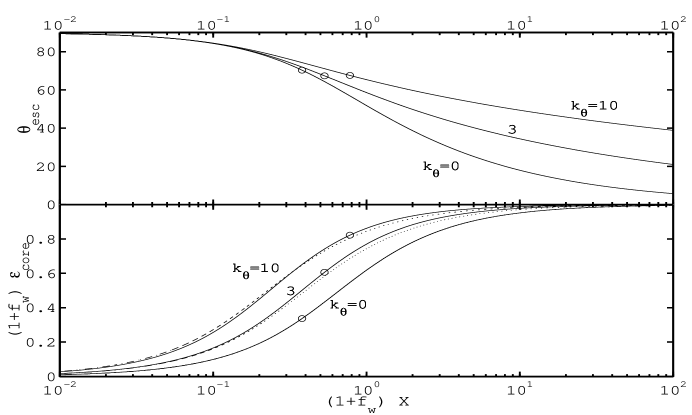
We find that the solution to this equation gives a star formation efficiency of the form in equation (31) with the replacement $X\rightarrow(1+H_{0})^{3/2}X$:

$$\varepsilon_{\rm core}\simeq\frac{2(1+H_{0})^{3/2}X}{1+[1+4(1+H_{0})^{3}(1+f_{w})^{2}X^{2}]^{1/2}}.$$ (44)

The validity of this approximation, depicted in Figure 1, implies that an increase in mean density by a factor of $(1+H_{0})$ is equivalent, as far as the efficiency is concerned, to a weakening of the momentum output in the wind by the factor $(1+H_{0})^{5/2}$. One of these factors of $(1+H_{0})$ is contained in $X$; it arises from the increase in escape velocity compared to a fixed value of $v_{w}$, as the mean density is increased. The other one and a half powers of $(1+H_{0})$ arise because of the increasing concentration of infalling material toward the equator, in the direction the wind is weakest. In the limit of a completely disk-like core [$(1+H_{0})\gg 1$], outflow occurs in all directions but along the equator ($\theta_{\rm esc}\rightarrow\pi/2$), but only the wind mass is ejected [$\varepsilon_{\rm core}\rightarrow 1/(1+f_{w})$].

Figure 1.— Core disruption and the efficiency of single star formation. Top: the angle $\theta_{\rm esc}$ (equation [43]) dividing accreted and ejected core material, which corresponds to an outflow velocity equal to the escape velocity of the collapsing core. For various values of the core flattening parameter $k_{\theta}$, the fiducial value $X=0.32(1+H_{0})$ (equation [42]; circles) leads to $\theta_{\rm esc}\simeq 67^{\circ}$ from the axis. Bottom: The efficiency $\varepsilon_{\rm core}$ of core collapse (equations [37] and [43]; solid lines) and an approximate formula (equation [44], dotted lines). Curves are plotted for $0<k_{\theta}<10$, corresponding to $1<(1+H_{0})<2$, where approximation (33) is known to be accurate.

5.3. The Initial Mass Function

Having determined $\varepsilon_{\rm core}$, it is possible to relate the IMF to the mass distribution of protostellar cores (Nakano et al. 1995). Let $d{{\cal N}}_{*}$ be the number of stars formed with masses in the mass range $m_{\star}$ to $m_{\star}+dm_{\star}$. Using a similar notation for the protostellar cores, we assume that they have a power-law distribution:

$$\frac{d{{\cal N}}_{\rm core}}{d\ln M_{\rm core}}\propto M_{\rm core}^{-{\alpha_{\rm core}}}.$$ (45)

Let

$${\varepsilon^{\prime}}\equiv\frac{d\ln\varepsilon_{\rm core}}{d\ln M_{\rm core}}.$$ (46)

If we approximate ${\varepsilon^{\prime}}$ as constant, then $\varepsilon_{\rm core}=m_{\star}/M_{\rm core}\propto M_{\rm core}^{\varepsilon^{\prime}}$. The IMF is then

$$\frac{d{{\cal N}}_{*}}{d\ln m_{\star}}=\frac{d{{\cal N}}_{\rm core}}{d\ln m_{\star}}\propto m_{\star}^{-{\alpha_{\rm core}}/(1+{\varepsilon^{\prime}})}.$$ (47)

To evaluate ${\varepsilon^{\prime}}$, we assume that the flattening parameter $H_{0}$ is independent of the core mass. Then $\varepsilon_{\rm core}$ depends on $X$, and it is straightforward to show from equation (44) that $d\ln\varepsilon_{\rm core}/d\ln X\leq 1$, and additionally that $d\ln\varepsilon_{\rm core}/d\ln X$ is a decreasing function of both $X$ and $(1+H_{0})$. From the definition (eq. 3), we see that $X$ depends directly on the properties of the core only through $v_{\rm esc}$. In principle, there could be an implicit dependence through $f_{w}v_{w}$, but we have argued in §3 that this is a constant for low-mass stars. Since the protostellar cores are gravitationally bound, their internal velocity dispersion is a fraction of their escape velocity, $\sigma\propto v_{\rm esc}$. Here, $\sigma$ includes both thermal and turbulent motions. Since protostellar cores are never colder than 10 K, $\sigma\geq 0.2~{}{\rm km\;s^{-1}}$: clumps must lie to the right of the circles in figure 1. Therefore, $\varepsilon_{\rm core}$ cannot be less than $0.3$ and $d\ln\varepsilon_{\rm core}/d\ln X$ cannot exceed $0.75$, the values for an unflattened core with $\sigma=0.2~{}{\rm km\;s^{-1}}$. Now, protostellar cores obey a line-width size relation of the form $\sigma\propto R_{\rm core}^{p}$ (Larson 1981). Since $v_{\rm esc}\propto(M_{\rm core}/R_{\rm core})^{1/2}$, we have $X\propto v_{\rm esc}\propto M_{\rm core}^{p/(2p+1)}$, so that

$${\varepsilon^{\prime}}=\frac{d\ln\varepsilon_{\rm core}}{d\ln X}\;\frac{d\ln X}{d\ln M_{\rm core}}\leq 0.75\frac{d\ln X}{d\ln M_{\rm core}}=0.75\frac{p}{2p+1}.$$ (48)

If the motions are primarily thermal, as we assumed in §5.2, then $p\simeq 0$ and therefore ${\varepsilon^{\prime}}\simeq 0$. On the other hand, if the motions are primarily non-thermal, then $p\simeq 1/2$ (Caselli & Myers 1995) and ${\varepsilon^{\prime}}\leq 0.19$. As a result, for all values of $\varepsilon_{\rm core}$, and regardless of whether the line width is primarily thermal or nonthermal, we have

$$0\leq{\varepsilon^{\prime}}\leq 0.19.$$ (49)

so that ${d{{\cal N}}_{*}}/{d\ln m_{\star}}\propto m_{\star}^{-(0.84-1){\alpha_{\rm core}}}$. Since in practice the thermal contribution to the line width is significant for low-mass cores, and since $d\ln\varepsilon_{\rm core}/d\ln X$ decreases as $\sigma$ (and thus $X$) increases, which reduces ${\varepsilon^{\prime}}$ for higher mass cores, we expect ${\varepsilon^{\prime}}\lesssim 0.1$ in general. Then,

$$\frac{d{{\cal N}}_{*}}{d\ln m_{\star}}\propto m_{\star}^{-(0.9-1){\alpha_{\rm core}}}.$$ (50)

Thus, over the mass range in which the core mass function is a power law and the star formation efficiency is determined by outflows, the slope of the IMF is expected quite generally to be just slightly flatter than than that of the protostellar cores. This theory does not address the IMF of high-mass stars, nor of cores sufficiently turbulent for fragmentation to occur during their collapse.

Although the above argument assumes a constant value of $H_{0}$ among cores, the result that the IMF is very close in slope to the core mass function is independent of this assumption. This follows from the fact that $0.3\leq\varepsilon_{\rm core}<1$ (figure 1). The two slopes cannot differ greatly if the stellar mass is always within a factor of three of the core mass.

Features in the core mass function (such as a peak) appear in the IMF at a mass that is smaller by the factor $\varepsilon_{\rm core}$.

5.4. Comparison with Observations

We have adopted a scenario in which a protostellar core is destroyed simultaneously by accretion onto a central star (near the equator) and by protostellar outflow (near the poles). This is broadly consistent with observations that indicate both processes are important in dissipating cores, such as those of Myers et al. (1988) and Ladd, Fuller, & Deane (1998). This geometry is confirmed by observations of the IRS 2 outflow source in Barnard 5 (Velusamy & Langer 1998), which clearly discern an equatorial inflow coexisting with an axial outflow.

Although we have not calculated the outflow structure in detail, the current theory implies the existence of a massive, slow, conical outflow that reaches the core escape velocity at about $23^{\circ}$ from the equator for the fiducial values of the parameters. This structure, which also appears in the theory of Li & Shu (1996), is likely to correspond to the massive, poorly collimated, $1~{}{\rm km\;s^{-1}}$ biconical outflow observed around T Tauri by Momose et al. (1996). The outflow cone observed by Velusamy and Langer extends to $\sim 27^{\circ}$ from the equator, in rough agreement with our prediction. More specific comparisons would require a solution to the problem of simultaneous infall and outflow, which is beyond the scope of this paper.

We derive values of $\varepsilon_{\rm core}$ that vary from $25\%$ to $75\%$ for the fiducial value $X=0.32(1+H_{0})$, for values of the core flattening parameter $0<k_{\theta}<10$ (i.e., $0<H_{0}<1$). Thus, we expect that spherical cores will lose three-quarters of their mass while forming a star, whereas cores at the upper end of the acceptable range of flattening (Li & Shu 1996) will lose only a quarter of their mass. The stellar initial mass function therefore depends not only on the mass function for cores, but also on the relative degrees of flattening of low and high-mass cores, and on changes of cores’ line widths with mass. Observations that indicate a strong similarity between the core and star mass functions (in both shape and peak mass), such as those of Motte et al. (1998), require that $\varepsilon_{\rm core}$ be roughly constant and of order unity. This is certainly consistent with the above theory, since $X(1+H_{0})^{3/2}$ is typically of order unity and $f_{w}$ is small, so that $\varepsilon_{\rm core}$ is indeed close to unity (eq. 44). Observations that indicate only similar slopes between the two distributions (e.g., Testi & Sargent 1998) do not constrain the value of $\varepsilon_{\rm core}$. They only require that it does not vary rapidly, a result that is consistent with the results of §5.3.

6. Instantaneous Star Formation Efficiency in Cluster-Forming Clumps

Clumps massive enough to form clusters of stars differ from the protostellar cores considered in the last section in several key respects. First, it is unlikely that there is a strong correlation between the geometry of the clump and the direction of the outflow. Provided the clump is not highly flattened, we can obtain a reasonable approximation to the effect of the wind by assuming that the clump is spherical [$Q(\mu)=1$]. As a result, the star formation efficiency is given by equation (27). Second, much of the mass of the clump is generally not involved in the formation of the star. An upper limit on the mass of a star that forms in the clump is given by the result for a protostellar core, in which all the mass is either accreted or ejected:

$$m_{\star}\leq m_{\rm\star,\,max}\equiv\varepsilon_{\rm core}M_{\rm cl}=\frac{2XM_{\rm cl}}{1+[1+4X^{2}(1+f_{w})^{2}]^{1/2}}.$$ (51)

There is no restriction on the formation of stars less massive than this, but stars with $m_{\star}<m_{\star,0}$ have outflows too weak to eject any matter from the clump.

A further difference between clumps and cores is that since the clumps contain the cores, the cores are generally significantly denser than the clumps in which they are embedded, and their free-fall times are correspondingly shorter. Insofar as the accretion time (and therefore $t_{w}$) is tied to the free-fall time, as in inside-out collapse models for star formation (Shu 1977), it follows that the star formation occurs on a time scale shorter than the free-fall time of the clump. In this case, the effect of gravity on the shell’s motion, which is characterized by the factor $c_{g}$ (eq. A13), is relatively minor:

$$c_{g}=\left(\frac{9-3{k_{\rho}}}{8-3{k_{\rho}}}\right)^{1/2},$$ (52)

which is of order unity for ${k_{\rho}}\leq 2$. We shall generally adopt ${k_{\rho}}=1$ for clumps, which is similar to or somewhat shallower than the clump structures inferred from observations (for instance, Yun & Clemens 1991, estimate $1<{k_{\rho}}\lesssim 2$ in Bok globules).

The final distinction between clumps and cores is that the clumps are generally not isothermal, and the rms velocity is often significantly greater than the thermal sound speed. Since both cores and star-forming clumps are gravitationally bound, it follows that the escape velocity is generally greater for clumps than for cores. Normalizing $v_{\rm esc}$ to 2 ${\rm km\;s^{-1}}$ for clumps, the efficiency parameter becomes

$$X=0.29\;\frac{\ln(2/\theta_{0})}{\ln 200}\left(\frac{v_{\rm esc}}{2\ {\rm km\;s^{-1}}}\right)\left(\frac{40\ {\rm km\;s^{-1}}}{f_{w}v_{w}}\right).$$ (53)

For $X=0.3$ and $f_{w}=0.2$, we have $m_{\rm\star,\,max}=0.27M_{\rm cl}$ from equation (51). Thus, for $M_{\rm cl}\lower 2.15277pt\hbox{$\;\buildrel>\over{\sim}\;$}500\,M_{\odot}$, a clump has enough mass to make a star with a mass up to $m_{\rm\star,\,max}\lower 2.15277pt\hbox{$\;\buildrel>\over{\sim}\;$}140\,M_{\odot}$, significantly above the upper mass cutoff in most star clusters in the Galaxy, even those that are far more massive than the clumps we are considering (Massey et al. 1995). Thus, we do not expect the formation of a single massive star to consume all the gas in a star-forming clump.

We shall neglect the loss of mass due to the winds themselves [$m_{w}(1-\phi_{w})\ll M_{\rm ej}$] for star formation within a clump. This approximation is justified below by the fact that $M_{\rm ej}\gg m_{w}$ for typical conditions ($m_{\star}\gg m_{\star,0}$). Furthermore, the accuracy of this approximation is improved somewhat by the fact that $\phi_{w}$ is typically about 0.5 in clumps (Matzner 1999). This implies that the error in $\varepsilon$ introduced by ignoring the contribution of $m_{w}$ to $M_{\rm ej}$ is only a couple percent when $\varepsilon\lesssim 50\%$, as we will find is typically the case in regions without massive stars.

To estimate $\varepsilon$ for a star-forming clump, we assume that all the star formation occurs at the center of the clump. As we shall see below, this apparently drastic approximation is in fact reasonably accurate. The critical angle for the escape of the swept-up shell is

$${\mu_{\rm esc}}=\left[1-\left(\frac{m_{\star}-m_{\star,0}}{XM_{\rm cl}}\right)\right]^{1/2}$$ (54)

from equations (17) and (25), provided, of course, that $m_{\star}\geq m_{\star,0}$. For $m_{\rm\star,\,max}\gg m_{\star}\gg m_{\star,0}$, as is typically the case, we have ${\mu_{\rm esc}}\simeq 1$ and equation (27) for the star formation efficiency simplifies to:

$$\frac{1}{\varepsilon}=1+1.72\;\frac{\ln 200}{\ln(2/\theta_{0})}\left(\frac{2\ {\rm km\;s^{-1}}}{v_{\rm esc}}\right)\left(\frac{f_{w}v_{w}}{40\ {\rm km\;s^{-1}}}\right).$$ (55)

Because we do not expect the intrinsic properties of a protostellar wind, $\theta_{0}$ and $f_{w}v_{w}$, to correlate with the escape velocity of the protostellar clump, equation (55) indicates that the efficiency with which clusters of low-mass stars are formed is a simple, increasing function of $v_{\rm esc}$. An escape velocity of order $2~{}{\rm km\;s^{-1}}$ leads to $\varepsilon\simeq 40\%$.

Equation (55) assumes that the mass ejected by each outflow can be tallied independently of other outflows. This can be verified by considering two outflows that occur simultaneously, which maximizes their interaction. If the angle between their axes is significantly greater than ${\theta_{\rm esc}}$ for either, then the momentum output from each is negligible within an angle ${\theta_{\rm esc}}$ of the other’s axis. Then, $M_{\rm ej}$ is given by equation (26) for each outflow individually. Alternatively, consider the case in which the outflows are completely aligned. They would then act as a single outflow whose momentum (and wind mass, assuming identical values of $v_{w}$) is the sum of its two components. So long as the combined mass of stars that forms simultaneously is still much less than $m_{\rm\star,\,max}\simeq M_{\rm cl}/3$, so that our assumption $1-{\mu_{\rm esc}}\ll 1$ still holds, equation (26) shows that $M_{\rm ej}$ is then the sum of the values it would take for each outflow individually. In either case, and thus quite generally, the relative timing and orientation of outflows is of little importance when estimating the mass they eject.

6.1. Numerical Models: Off-Center, Ionization-Regulated Star Formation in Clusters

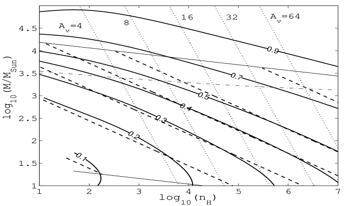
We wish to assess the accuracy of equation (55), in which we assumed that each star forms at the exact center of its clump. In this section, we present calculations of $\varepsilon$ for off-center star formation. As above, we assume that the clump is spherically symmetric with ${\rho_{\rm cl}}\propto r^{-{k_{\rho}}}$; we set ${k_{\rho}}=1$. We draw all stars from the same initial mass function independently of their position within the clump, and orient their outflow axes at random. The IMF is taken to be a Miller-Scalo log-normal distribution, with a lower cutoff at $0.057~{}{\rm M}_{\mathord{\odot}}$, so that $\overline{m}_{\star}=0.5~{}{\rm M}_{\mathord{\odot}}$. We take stars to be formed in the clump at a local rate $t_{g\star}^{-1}\equiv\dot{M}_{\star}/M_{\rm cl}$ equal to the ambipolar diffusion rate $t_{\rm AD}^{-1}$, as in the photoionization-regulation model of McKee (1989). Because $t_{\rm AD}\propto t_{\rm ff}$ if cosmic-ray ionization prevails, we take the star formation rate to vary with the free-fall rate in the region of high extinction. The ambipolar diffusion rate decreases sharply due to far-ultraviolet ionization as the visual extinction to the surface $A_{Vs}$ falls below about four magnitudes. Although this transition can be described analytically (Matzner et al. 2000), for simplicity we shall take the transition to be sudden: $t_{g\star}(r)^{-1}\propto t_{\rm ff}(r)^{-1}\propto\rho(r)^{1/2}$ if $A_{Vs}>4$ and $t_{g\star}^{-1}=0$ if $A_{Vs}<4$.

For each star, a grid of solid angles is constructed around its outflow axis. The wind momentum is distributed on this grid, whose resolution is concentrated toward the axis for improved numerical accuracy. The clump mass per solid angle is also computed, using the distance from the newborn star to the center of the clump, and using the angle between its axis and the radial direction. The ratio between $dp_{w}/d\Omega$ and $dM_{\rm cl}/d\Omega$ gives the shell velocity at the clump surface; this is compared to $c_{g}v_{\rm esc}$, and the total ejected mass is tallied. Thus, the effect of gravity is included as an overall factor, rather than considered in the motion of each outflow element.

In Figure 2, we compare the results of this numerical investigation to our analytical formulae. Allowing for distributed star formation and averaging over the initial mass function changes the estimated efficiencies appreciably only when the assumption $m_{\star,0}\ll\overline{m}_{\star}\ll m_{\rm\star,\,max}$ breaks down (near the thin lines that represent these limits in Figure 2). For instance, the curvature of the numerical contours of $\varepsilon$ away from the analytical contours at the bottom of the plot can be attributed to the smallness of $m_{\rm\star,\,max}/\overline{m}_{\star}$ in that region. We have also compared to a calculation of $\varepsilon$ that averages over the stellar initial mass function but assumes each star forms at the center: this reproduces the off-center calculation almost exactly, except for $m_{\star,0}>\overline{m}_{\star}$. In general, assuming that each star forms at the center yields an excellent approximation of the star formation efficiency.

Figure 2.— Estimates of the instantaneous star formation efficiency $\varepsilon$ due to protostellar outflows. Dashed lines: analytical estimate, equation (55). Solid lines: Numerical evaluation of the same quantity in a protostellar clump with the structure $\rho\propto r^{-1}$ and gas conversion rate scaling as $\rho^{1/2}$ in regions extinguished by more than four magnitudes from the surface. In this calculation, the effect of gravity on outflow motions has been included with an overall correction factor $c_{g}$ (equation [52]). Dotted lines indicate the mean extinction of the clump. Above the dash-dot line, stars more massive than $20~{}{\rm M}_{\mathord{\odot}}$ are likely to form; our estimates are therefore only rough upper limits in this region. Below the lower thin line, $m_{\rm\star,\,max}$ is less than twice the mean stellar mass; above the upper thin line, $m_{\star,0}$ exceeds the mean stellar mass. The analytical approximation requires $m_{\star,0}\ll\overline{m}_{\star}\ll m_{\rm\star,\,max}$, and breaks down near the thin lines.

6.2. Comparison with Observations

The above theory implies that the clumps that give rise to clusters of low-mass stars, like those in L1630 ($n_{H}\sim 10^{4}~{}{\rm cm}^{-3}$, $200<M_{\rm cl}<500~{}{\rm M}_{\mathord{\odot}}$; Lada 1992), form each star at an efficiency $30\%\lesssim\varepsilon\lesssim 40\%$. This range of efficiencies agrees with the theoretical arguments by Mathieu (1983) and Elmegreen (1983), who compared the properties of known embedded and revealed bound clusters of similar masses and determined that star formation efficiencies of about $30\%$ or $55\%$ would be necessary for the embedded bound clusters to evolve into the revealed bound clusters, in the respective limits of slow or rapid gas dispersal.

As described in §2, the observable efficiency is not the instantaneous efficiency, $\varepsilon$, but instead the ratio of stellar to total mass, ${\rm SFE}$. Whereas $\varepsilon$ is a simple function of the current escape velocity from the system (eq. 55), ${\rm SFE}$ is expected to vary from zero to unity as stars form and gas is dissipated; $\varepsilon$ is only a rough estimate for the characteristic value of ${\rm SFE}$ in the midst of this process. Without knowing the evolution of the system, it is therefore difficult to compare an observation of ${\rm SFE}$ to our prediction of $\varepsilon$. In L1630, the observations of Lada (1992) imply ${\rm SFE}\simeq 7\%$ (NGC 2023 and LBS 23), $19\%$ (NGC 2071), and $42\%$ (NGC 2024 and 2068) if one assumes each detected source signifies $1~{}{\rm M}_{\mathord{\odot}}$ of stellar material. This assumption is relatively uncertain due to variable extinction in the area, luminosity variation in the embedded sources, and the completeness limit of the survey. If instead each source signified the mean stellar mass ($\sim 0.5~{}{\rm M}_{\mathord{\odot}}$), the inferred efficiencies would be about a factor of two lower. A direct comparison with theory is therefore difficult for both theoretical and experimental reasons, but it is encouraging that there is rough agreement for the richer clusters, which may be more evolved.

Onishi et al. (1998) have conducted a survey in Taurus for dense gas and young stellar objects in various phases of evolution, in order to ascertain the evolutionary sequence leading to cluster formation. They find that only those clumps (and all those clumps) with mean visual extinction $A_{V}>8~{}{\rm mag}$ are actively forming stars, in agreement with the theoretical prediction of McKee (1989). However, some clumps of lower extinction contain more evolved objects that presumably formed while the column density was above this threshold. Considering the decrease in column density to correspond to a loss of gas mass, and multiplying by the mean area per star, these authors estimate that about $4~{}{\rm M}_{\mathord{\odot}}$ is lost per observed object, i.e., $\varepsilon({\rm obs})\sim 11\%$ if each object represents $0.5~{}{\rm M}_{\mathord{\odot}}$ of stellar material. This observational determination of efficiency is also quite uncertain. It should be considered a lower limit for several reasons: the stellar sample is likely to miss a significant fraction of weak-line T Tauri stars (Briceño et al. 1999, 1998); stars may have drifted away from the older clumps; and the decrease in column density could be partly due to an expansion of the clumps over time. Moreover, the currently star-forming clumps have not created their full complement of stars: on average, one might expect about half the stars to have been born by now, in which case $\varepsilon({\rm obs})\sim 22\%$. The star-forming clumps in this sample have escape velocities ranging from $0.8$ to $1.4~{}{\rm km\;s^{-1}}$, for which we estimate $\varepsilon\sim 25\pm 5\%$ from equation (55). Again, the theory predicts efficiencies similar to the values inferred from observation.

7. Conclusions

The star formation efficiency is a fundamental property of the process of star formation. Star formation is often said to be inefficient because it occurs much more slowly than it potentially could, as discussed in the Introduction. However, when defined in terms of the fraction of the available mass that goes into stars, it is rather high—at least for low-mass stars. For such stars, the efficiency is determined by the powerful protostellar winds that accompany the formation of the star. These winds produce a total momentum per unit mass of star formed of order $m_{w}v_{w}/m_{\star}\equiv f_{w}v_{w}\simeq 40\,{\rm km\;s^{-1}}$. If this momentum were transferred to the surrounding gas isotropically, then the mass ejected would be much greater than the mass that goes into the star, and the efficiency would be low (Nakano et al 1995). In fact, however, protostellar winds are highly collimated. To determine the star formation efficiency resulting from collimated outflows, we assumed: (1) the interaction between the protostellar wind and the ambient gas is mediated by thin, radiative shocks that lead to radial outflow; (2) except possibly near the wind axis, the mass of the wind is small compared with the mass swept up by the wind shock; and (3) there is an angle ${\theta_{\rm esc}}$ relative to the wind axis inside of which all mass is ejected and outside of which mass can accrete toward the central source, with a fraction $f_{w}/(1+f_{w})$ going into the protostellar wind. Assumptions (1) and (2) are consistent with observations of the momentum distribution in protostellar outflows (Matzner & McKee 1999).

We additionally assumed (4) that $f_{w}v_{w}$ is the same among stars of different masses. This assumption, which is justified by the fact that deuterium burning regulates protostars’ escape velocity (Stahler 1988) and thus the wind velocity (Shu et al. 1994), leads to an estimate of the star formation efficiency that is the same for most stars and depends only on the escape velocity of the region (eq. [55]). If this assumption did not hold, $\varepsilon$ would vary among stars. However the conclusions of § 6 would still be valid, as the star formation efficiency for a clump is an average over the IMF.

The principal effect of wind collimation on the momentum transfer to the ambient gas is to concentrate the momentum in a mass that is smaller than in the isotropic case by a factor of order $1/\ln(2/\theta_{0})$, where $\theta_{0}\sim 10^{-2}$ is the size of the central region of the outflow (eq. 11). Gas is ejected if its velocity exceeds the escape velocity, $v_{\rm esc}$; as a result, the mass ejected is given by $M_{\rm ej}v_{\rm esc}\sim m_{\star}f_{w}v_{w}/\ln(2/\theta_{0})$. If the ejected mass is larger than the protostellar mass, then the star formation efficiency is approximately

$$\varepsilon\simeq\frac{m_{\star}}{M_{\rm ej}}\simeq\frac{v_{\rm esc}\ln(2/\theta_{0})}{f_{w}v_{w}}.$$ (56)

This result, which applies both to the formation of individual stars in a core or the formation of a cluster of stars in a star-forming clump, shows that the efficiency of formation of low-mass stars is

• independent of the mass of the star; and

• only weakly dependent on the properties of the core or clump, through $v_{\rm esc}\propto(M_{\rm cl}/R_{\rm cl})^{1/2}\propto M_{\rm cl}^{1/3}{\rho_{\rm cl}}^{1/6}$.

Consequently, the efficiency is only weakly dependent on the geometry of the star-forming region and the location of the outflow source within it, as the results of §§5 and 6.1 demonstrate. These conclusions are in qualitative agreement with those of Nakano et al. (1995), but our inclusion of the collimation of the outflows increases the estimated star formation efficiency by about an order of magnitude, so that $\varepsilon\sim 0.25-0.75$.

We have evaluated the star formation efficiency separately for protostellar cores and for star-forming clumps. Protostellar cores are expected to be flattened in a direction perpendicular to the outflow; since the outflow and inflow are in different directions, the star formation efficiency is increased over the case of an isotropic ambient medium. We evaluated this effect quantitatively using the Li-Shu (1996) model of isothermal, magnetized protostellar cores (see Fig. 1). Because $\varepsilon$ is independent of the stellar mass and only weakly dependent on the core mass, we predict (in agreement with Nakano et al 1995) that the initial mass function is just slightly flatter than the mass distribution of protostellar cores, with a power-law index $(0.9-1){\alpha_{\rm core}}$.

Our model differs from most previous proposals in that the wind acts to limit the fraction of the mass that can accrete, but does not cause accretion to shut off entirely. This is consistent with the fact that accretion is necessary to drive a powerful wind. Instead, accretion terminates because only a finite reservoir of gas is available. In contrast to the proposal of Velusamy & Langer (1998), for instance, the angle dividing accreted and ejected material takes a characteristic value during the main accretion phase. Variations of $\theta_{\rm esc}$ may result from a decline in the accretion rate, but do not cause it.

Another distinction of the theory presented here is that the division between accretion and ejection occurs in swept-up material traveling outward at the escape velocity – material outside the region of significant infall and far outside the centrifugal radius. Therefore the complicated interaction among outflow, infall and rotation, which determines the shape of the outflow cavity at its base, does not affect the efficiency. All of the material at the base of the flow is destined to accrete, for rotational flattening and infall only act to lessen the effect of the wind.

We have found that the star formation efficiency is controlled by the efficiency parameter $X$ (equation [3]), and in the case of magnetically flattened protostellar cores, also by the flattening parameter $(1+H_{0})$. The factors that introduce uncertainty into the theory are primarily those that affect $X$. For instance, the factor $c_{g}$ that corrects for the effect of gravity on the outflow motions is well-understood for clumps of hydrogen number density below $10^{5}~{}{\rm cm}^{-3}$, in which winds are impulsive. As we discuss in §3, we expect that winds are approximately impulsive for higher mean densities as well; however, the accuracy of this approximation is difficult to assess. For the formation of an individual star, the wind duration is longer than the free-fall time of the core. This raises the question, addressed in §A.2 of the Appendix, of what happens to material when it reaches the core’s surface. The results presented in §5 presume that the shocked shell decouples from the wind outside the core; however, equation (A17) shows that $c_{g}$ would be three times lower in the opposite limit of perfect coupling.

A second source of uncertainty is the parameter $f_{w}v_{w}$ that relates a star’s final mass to the momentum of its wind. As discussed in §3, our value, $f_{w}v_{w}=40~{}{\rm km\;s^{-1}}$, is consistent with current observational and theoretical estimates; however, both are somewhat uncertain.

Our estimate of the effective broadening angle, $\theta_{0}$, of protostellar winds is also not precise. Matzner & McKee (1999) estimate $\theta_{0}\simeq 10^{-2}$ by comparing the mass-velocity distributions of outflows to the predictions of a simple model for their dynamics, and by requiring that the model fit observations for realistic inclinations of the wind axis to the line of sight. Note that $\theta_{0}$ enters logarithmically in the efficiency parameter $X$, as $\log(2/\theta_{0})$; therefore, we consider it a minor source of uncertainty as compared to $f_{w}v_{w}$. However, because the intensity of protostellar winds along their axes is proportional to $\theta_{0}^{-2}$, this parameter plays a more important role in determining the minimum stellar mass $m_{\star,0}$ capable of ejecting any mass. The efficiency increases dramatically (and equation [55] breaks down) for clump masses large enough that $m_{\star,0}$ becomes comparable to the mean stellar mass. For $\theta_{0}=10^{-2}$, this happens when $M_{\rm cl}\gtrsim 10^{4}~{}{\rm M}_{\mathord{\odot}}$ (the upper thin line in figure 2). Another condition for the validity of our theory is that massive stars do not dominate the ejection of mass; as shown by the dash-dot line in that figure, we expect that to happen when $M_{\rm cl}\gtrsim 10^{3.5}~{}{\rm M}_{\mathord{\odot}}$. Thus for $\theta_{0}=10^{-2}$, the former is the more restrictive criterion; if $\theta_{0}$ were greater than about $10^{-1.5}$, the latter would be.

Lastly, we expect that the assumption of radial motion is not perfect. Most likely, this implies that our estimate of $X$ should be adjusted by a correction factor of order unity.

For star-forming clumps, we found that the star-formation efficiency is typically somewhat less than 0.5, although slight variations in the parameters can bring $\varepsilon$ above 0.5. As discussed in §1.2, such high efficiencies might be expected to leave the cluster gravitationally bound. To show why most clusters are unbound, we must consider the dynamics of cluster formation, a topic we address in a future paper.

Appendix A Effect of gravity on outflow motions

Because $v_{\rm esc}$ marks the boundary between ejected and retained material, and because gravity is important for the dynamics of a shell if its mean velocity is about $v_{\rm esc}$, we wish to refine our estimate of the escape criterion accounting for gravity.

Assume that a star forms at the center of the clump, and that the clump’s gravitational potential is not perturbed by the passage of the outflow. Take the distribution of momentum injection to vary with angle away from the outflow axis as

$$\frac{d\dot{p}_{w}}{d\Omega}=\frac{\dot{p}_{w}P(\mu)}{4\pi};$$ (A1)

our model for $P(\mu)$ is given in equation (10). We take the distribution of clump density to be

$${\rho_{\rm cl}}=\rho_{01}Q(\mu)r^{-{k_{\rho}}}$$ (A2)

for $0<r<R_{\rm cl}$, where the normalization of the angular distribution of the density is $\int_{0}^{1}Q(\mu)d\mu=1$. The mass per unit solid angle enclosed within radius $r$ is therefore

$$\frac{dM_{\rm cl}}{d\Omega}=\frac{1}{4\pi}M_{\rm cl}(r)Q(\mu)=\frac{c_{M}}{4\pi}Q(\mu)r^{3-{k_{\rho}}},$$ (A3)

where the total mass inside $r$ is $M_{\rm cl}(r)=c_{M}r^{3-{k_{\rho}}}$, and $c_{M}\equiv 4\pi\rho_{01}/(3-{k_{\rho}})$.

To determine the condition for the wind to eject material from the surrounding clump or core, we make several approximations (§4): We assume radial, momentum-conserving flow, and we neglect $dm_{w}/d\Omega$ compared with $dM_{\rm cl}/d\Omega$ in regions in which the velocity of the shell is small compared with the wind velocity, $v_{s}\ll v_{w}$. In addition, we adopt the monopole approximation for gravity, which is generally quite good, even for flattened distributions (Li & Shu 1997). The equation of motion for a sector of the shell is then

$$\frac{d}{dt}\frac{dM_{\rm cl}}{d\Omega}v_{s}=\frac{d\dot{p}_{w}}{d\Omega}-\frac{GM}{r^{2}}\frac{dM}{d\Omega},$$ (A4)

or

$$\frac{d}{dt}M_{\rm cl}(r)v_{s}=\frac{P(\mu)}{Q(\mu)}{\dot{p}_{w}}-\frac{GM^{2}}{r^{2}},$$ (A5)

where we have divided through by $Q(\mu)$. In the monopole approximation, the kinematics of the shocked shell depend only on the ratio $P(\mu)/Q(\mu)$, not on either one independently.

If we neglect the effect of gravity on the propagation of the shock, as in the main text, equation (A5) integrates to give

$$M_{\rm cl}v_{s}=\frac{P(\mu)}{Q(\mu)}p_{w}(t).$$ (A6)

Usually, we shall adopt the criterion that a sector of the shell will escape from the clump if its velocity exceeds the escape velocity. The critical angle at which escape is marginally possible, ${\theta_{\rm esc}}=\cos^{-1}{\mu_{\rm esc}}$, is then determined by setting $p_{w}(t)=p_{w}$, the total wind momentum, and $v_{s}=v_{\rm esc}$ in equation (A6). Including the effect of gravity on the dynamics of the shell increases the required momentum by a factor $c_{g}\geq 1$ that we shall determine below:

$$\frac{P({\mu_{\rm esc}})}{Q({\mu_{\rm esc}})}p_{w}=c_{g}M_{\rm cl}v_{\rm esc}.$$ (A7)

To solve for the dynamics of the shock in the clump including the effects of gravity, we express $M_{\rm cl}(r)$ as $c_{M}r^{3-{k_{\rho}}}$ and $d/dt$ as $v_{s}d/dr$. Equation (A4) then becomes

$$c_{M}v_{s}\frac{d}{dr}v_{s}r^{3-{k_{\rho}}}=\frac{P(\mu)}{Q(\mu)}\dot{p}_{w}-Gc_{M}^{2}r^{4-{k_{\rho}}}.$$ (A8)

We now introduce the variables $x\equiv r^{4-{k_{\rho}}}$ and $y\equiv r^{3-{k_{\rho}}}v_{s}$; in terms of these variables, equation (A8) becomes

$$\frac{4-{k_{\rho}}}{2}c_{M}\frac{dy^{2}}{dx}=\frac{P(\mu)}{Q(\mu)}\dot{p}_{w}-Gc_{M}^{2}x^{(4-2{k_{\rho}})/(4-{k_{\rho}})}.$$ (A9)

Integrating, and transforming back to radius and velocity from $x$ and $y$, we find

$$M_{\rm cl}v_{s}^{2}=\frac{2}{4-{k_{\rho}}}\frac{P(\mu)}{Q(\mu)}\dot{p}_{w}r-\frac{M_{\rm cl}v_{\rm esc}(r)^{2}}{8-3{k_{\rho}}}+\frac{C}{M_{\rm cl}},$$ (A10)

where we have defined $v_{\rm esc}(r)\equiv\sqrt{2GM_{\rm cl}(r)/r}$ as the local escape velocity [so that $v_{\rm esc}(R_{\rm cl})=v_{\rm esc}$], and $C$ is a constant of integration.

A.1. Impulsive Winds

Consider the case that the wind momentum is injected impulsively, i.e, $t_{w}\ll t_{\rm ff}$. Then, $\dot{p}_{w}=0$ during the shell’s expansion, so that (multiplying through by $M_{\rm cl}$)

$$M_{\rm cl}^{2}v_{s}^{2}=-\frac{M_{\rm cl}^{2}v_{\rm esc}(r)^{2}}{8-3{k_{\rho}}}+C.$$ (A11)

Evaluating this equation at $r=0$, where $M_{\rm cl}v_{\rm esc}(r)=0$, we find $M_{\rm cl}Q(\mu)v_{s}=p_{w}P(\mu)$; therefore $C=[p_{w}P(\mu)/Q(\mu)]^{2}$, and

$$M_{\rm cl}^{2}v_{s}^{2}=\left[\frac{P(\mu)}{Q(\mu)}p_{w}\right]^{2}-\frac{M_{\rm cl}^{2}v_{\rm esc}(r)^{2}}{8-3{k_{\rho}}}.$$ (A12)

The condition for the escape is $v_{s}(R_{\rm cl})>v_{\rm esc}$, or

$$\frac{P(\mu)}{Q(\mu)}p_{w}>\left(\frac{9-3{k_{\rho}}}{8-3{k_{\rho}}}\right)^{1/2}M_{\rm cl}v_{\rm esc}.$$ (A13)

Thus, in this case the factor by which the critical wind force must be enhanced to offset the effects of gravity on the dynamics of the shell is $c_{g}=[(9-3{k_{\rho}})/(8-3{k_{\rho}})]^{1/2}$ (cf eq. A7).

A.2. Steady Winds

Next, consider what happens if the wind momentum injection is constant throughout the expansion of the shell, so that $\dot{p}_{w}$ maintains the steady value $p_{w}/t_{w}$. Furthermore, let us suppose that the wind continues to inject momentum after the shell breaks out of the clump. Then, a naïve estimate for the criterion for escape is that the wind force overcome gravity at the clump surface,

$$\frac{P(\mu)}{Q(\mu)}p_{w}\lower 2.15277pt\hbox{$\;\buildrel>\over{\sim}\;$}\frac{GM_{\rm cl}^{2}t_{w}}{R_{\rm cl}^{2}}=\frac{\pi t_{w}}{4t_{\rm ff}}M_{\rm cl}v_{\rm esc}.$$ (A14)

This estimate gives $c_{g}=(\pi/4)(t_{w}/t_{\rm ff})$ for the factor by which the momentum in the wind must be enhanced to overcome the effects of gravity on the shell dynamics. This factor is large when $t_{w}\gg t_{\rm ff}$ since only the momentum delivered in a time of order $t_{\rm ff}$ is effective in ejecting the shell. In fact, the condition $c_{g}\geq 1$ sets a lower bound on the value of $t_{w}/t_{\rm ff}$ for a steady wind.

Consider the dynamics of the outflow shell after it has broken free of the clump, so that its mass is constant. Then, since we are assuming that $\dot{p}_{w}$ is constant in time, we can integrate equation (A5) directly, using $d/dt=v_{s}d/dr$:

$$E(r)-E(R_{\rm cl})=\frac{P(\mu)}{Q(\mu)}\dot{p}_{w}(r-R_{\rm cl}),$$ (A15)

where $E(r)=M_{\rm cl}v_{s}^{2}/2-GM_{\rm cl}^{2}/r$ is the energy of the shell and $E(R_{\rm cl})$ is its energy at the clump surface. If the wind were no longer blowing, the shell’s energy would be constant and positive energy ($v_{s}^{2}>GM_{\rm cl}^{2}/r$) would lead to escape. However, we are assuming that the wind continues to blow well past the time that the shocked shell reaches the clump surface. In this case, the shell might escape even if it has negative energy, because of the wind force. (Below, we shall consider the case that the outflow decouples from the wind after breaking out.)

We shall evaluate $v_{s}(R_{\rm cl})$ using equation (A10), and then use equation (A15) to determine the criterion for escape. We readily see that $C=0$ for a steady wind, for all the other terms in equation (A10) are zero at the origin; therefore,

$$M_{\rm cl}v_{s}^{2}=\frac{2}{4-{k_{\rho}}}\frac{p_{w}rP(\mu)}{t_{w}Q(\mu)}-\frac{M_{\rm cl}v_{\rm esc}(r)^{2}}{8-3{k_{\rho}}}~{}~{}~{}~{}~{}{(r\leq R_{\rm cl})}.$$ (A16)

Using the value of $E(R_{\rm cl})$ from this in equation (A15), and requiring that $dE(r)>-GM_{\rm cl}dM_{\rm cl}/r$ [so that $v_{s}^{2}(r)>0$] for all $r$, we find the critical value of the wind force:

$$\frac{P(\mu)}{Q(\mu)}p_{w}>\left(\frac{4-{k_{\rho}}}{3-{k_{\rho}}}\right)^{2}\left\{1-\left[\frac{5-2{k_{\rho}}}{(8-3{k_{\rho}})(4-{k_{\rho}})}\right]^{1/2}\right\}^{2}\times\frac{\pi t_{w}}{4t_{\rm ff}}M_{\rm cl}v_{\rm esc}.$$ (A17)

This more precise wind force criterion is $35\%$ and $31\%$ lower than the simple estimate of equation (A14) for ${k_{\rho}}=0$ and ${k_{\rho}}=1$, respectively. The two agree exactly for ${k_{\rho}}=2$, because gravity and wind force scale in the same manner inside the clump in that case. This implies that the shell velocity at the surface vanishes if the wind force equals the critical value if ${k_{\rho}}=2$, exactly as we assumed in estimate (A14).

Equations (A14) – (A17) assume that the wind continues to deposit momentum into the shell efficiently, even after the outflow has emerged from the clump. There are two reasons that this assumption may be incorrect, which make the above estimates lower limits for the critical wind force. First, if $t_{w}$ is not too much longer than $t_{\rm ff}$, there is the possibility that the wind force will taper off before the shell has achieved escape velocity. Second, there is the possibility that the shell will be disrupted by a thin-shell instability. The former effect can be ignored, because it is only important when $t_{w}\simeq t_{\rm ff}$. The latter is more serious, as it would remove the supporting effect of the wind (partially or completely) once the instability set in.

Shock-bounded thin shells are subject to nonlinear instabilities (e.g., Vishniac 1994); these are expected to become stronger if the dense fluid (the ambient gas, in this case) is “upward”, i.e., if the shell accelerates, or at least decelerates more slowly than gravity would predict (E. T. Vishniac, private communication). Writing out $d(dM_{\rm cl}/d\Omega)/dt$ as $r^{2}v_{s}{\rho_{\rm cl}}$ and $d\dot{p}_{w}/d\Omega$ as $\rho_{w}v_{w}^{2}r^{2}$, we find from equation (A4) that the difference between the actual acceleration and gravity is

$$\frac{dv_{s}}{dt}+\frac{GM_{\rm cl}}{r^{2}}=\frac{r^{2}}{dM_{\rm cl}/d\Omega}(\rho_{w}v_{w}^{2}-{\rho_{\rm cl}}v_{s}^{2}).$$ (A18)

Since gravity is an additive term in the acceleration, we see that the shell decelerates more slowly than gravity would predict (and is unstable) if the same shell would accelerate, were gravity suddenly turned off. Equation (A18) shows that this only occurs if the ram pressure in the wind exceeds the ram pressure of the ambient gas. For a steady wind, this requires that the ambient medium must steepen so that ${k_{\rho}}>2$ (declining winds would require even steeper profiles). We therefore expect that shells might become partially decoupled from their winds as they emerge from a clump, not before.

Although this instability is nonlinear, and may be suppressed by magnetic fields in the outflow shell or in the wind, we can obtain an upper limit to the critical wind force if we assume that outflows decouple entirely from their winds after breakout. Then, the criterion for ejection is once again $v_{s}(R_{\rm cl})>v_{\rm esc}$. From equation (A16), this requires

$$\frac{P(\mu)}{Q(\mu)}p_{w}>(4-{k_{\rho}})\frac{9-3{k_{\rho}}}{8-3{k_{\rho}}}\times\frac{GM_{\rm cl}^{2}t_{w}}{R_{\rm cl}^{2}}=(4-{k_{\rho}})\frac{9-3{k_{\rho}}}{8-3{k_{\rho}}}\times\frac{\pi t_{w}}{4t_{\rm ff}}M_{\rm cl}v_{\rm esc}.$$ (A19)

The factor $c_{g}$ in this case is the coefficient of $M_{\rm cl}v_{\rm esc}$ in the equation above. We see that the wind force required to eject the shell is much stronger if the shell decouples from the wind after breakout than if the wind continues to provide support, the factor between equations (A17) and (A19) being seven or three if ${k_{\rho}}$ is zero or two, respectively.

References

- Adams & Fatuzzo (1996) Adams, F. C. & Fatuzzo, M. 1996, ApJ, 464, 256
- Adams et al. (1989) Adams, F. C., Ruden, S. P., & Shu, F. H. 1989, ApJ, 347, 959
- Arce & Goodman (2000) Arce, H. & Goodman, A. 2000, in prep.
- Bally & Duvert (1994) Bally, J.and Castets, A. & Duvert, G. 1994, ApJ, 423, 310
- Bally et al. (1999) Bally, J., Reipurth, B., Lada, C. J., & Billawala, Y. 1999, AJ, 117, 410
- Benson & Myers (1989) Benson, P. J. & Myers, P. C. 1989, ApJS, 71, 89
- Bertoldi & McKee (1996) Bertoldi, F. & McKee, C. F. Self-regulated star formation in molecular clouds (Amazing Light: A Volume Dedicated to C.H. Townes on his 80th Birthday, ed. R.Y.Chiao (New York: Springer)), 41
- Bontemps et al. (1996) Bontemps, S., Andre, P., Terebey, S., & Cabrit, S. 1996, A&A, 311, 858
- Briceño et al. (1999) Briceño, C., Calvet, N., Kenyon, S., & Hartmann, L. 1999, AJ, 118, 1354
- Briceño et al. (1998) Briceño, C., Hartmann, L., Stauffer, J., & Martín, E. 1998, AJ, 115, 2074
- Caselli & Myers (1995) Caselli, P. & Myers, P. C. 1995, ApJ, 446, 665
- Elmegreen (1983) Elmegreen, B. G. 1983, MNRAS, 203, 1011
- Goldsmith et al. (1986) Goldsmith, P. F., Langer, W. D., & Wilson, R. W. 1986, ApJ, 303, L11
- Hills (1980) Hills, J. G. 1980, ApJ, 235, 986
- Lada & Gautier (1982) Lada, C. J. & Gautier, T. N., I. 1982, ApJ, 261, 161
- Lada et al. (1984) Lada, C. J., Margulis, M., & Dearborn, D. 1984, ApJ, 285, 141
- Lada (1992) Lada, E. A. 1992, ApJ, 393, L25
- Lada et al. (1991) Lada, E. A., Evans, Neal J., I., Depoy, D. L., & Gatley, I. 1991, ApJ, 371, 171
- Ladd et al. (1998) Ladd, E. F., Fuller, G. A., & Deane, J. R. 1998, ApJ, 495, 871
- Langer et al. (1986) Langer, W. D., Frerking, M. A., & Wilson, R. W. 1986, ApJ, 306, L29
- Larson (1981) Larson, R. B. 1981, MNRAS, 194, 809
- Lee et al. (1999) Lee, C. W., Myers, P. C., & Tafalla, M. 1999, ApJ, 526, 788
- Levreault (1984) Levreault, R. M. 1984, ApJ, 277, 634
- Li et al. (1997) Li, W., Evans, Neal J., I., & Lada, E. A. 1997, ApJ, 488, 277
- Li (1998) Li, Z.-Y. 1998, ApJ, 497, 850
- Li & Shu (1996) Li, Z.-Y. & Shu, F. H. 1996, ApJ, 472, 211
- Li & Shu (1997) Li, Z.-Y. & Shu, F. H. 1997, ApJ, 475, 237
- Massey et al. (1995) Massey, P., Johnson, K., & DeGioia-Eastwood, K. 1995, ApJ, 454, 151
- Mathieu (1983) Mathieu, R. D. 1983, ApJ, 267, L97
- Matzner et al. (2000) Matzner, C., Bertoldi, F., & McKee, C. F. 2000, in prep.
- Matzner (1999) Matzner, C. D. 1999, PhD thesis, U. C. Berkeley
- Matzner & McKee (1999) Matzner, C. D. & McKee, C. F. 1999, ApJ, 526, L109
- McKee (1989) McKee, C. F. 1989, ApJ, 345, 782
- McKee & Williams (1997) McKee, C. F. & Williams, J. P. 1997, ApJ, 476, 144
- Miller & Scalo (1978) Miller, G. E. & Scalo, J. M. 1978, PASP, 90, 506
- Momose et al. (1996) Momose, M., Ohashi, N., Kawabe, R., Hayashi, M., & Nakano, T. 1996, ApJ, 470, 1001
- Motte et al. (1998) Motte, F., André, P., & Neri, R. 1998, A&A, 336, 150
- Mouschovias (1991) Mouschovias, T. C. 1991, ApJ, 373, 169
- Myers et al. (1988) Myers, P. C., Heyer, M., Snell, R. L., & Goldsmith, P. F. 1988, ApJ, 324, 907
- Najita & Shu (1994) Najita, J. R. & Shu, F. H. 1994, ApJ, 429, 808
- Nakano et al. (1995) Nakano, T., Hasegawa, T., & Norman, C. 1995, ApJ, 450, 183
- Norman & Silk (1980) Norman, C. & Silk, J. 1980, ApJ, 238, 158
- Onishi et al. (1998) Onishi, T., Mizuno, A., Kawamura, A., Ogawa, H., & Fukui, Y. 1998, ApJ, 502, 296
- Pelletier & Pudritz (1992) Pelletier, G. & Pudritz, R. E. 1992, ApJ, 394, 117
- Reipurth et al. (1997) Reipurth, B., Bally, J., & Devine, D. 1997, AJ, 114, 2708
- Safier et al. (1997) Safier, P. N., McKee, C. F., & Stahler, S. W. 1997, ApJ, 485, 660
- Shu et al. (1994) Shu, F., Najita, J., Ostriker, E., Wilkin, F., Ruden, S., & Lizano, S. 1994, ApJ, 429, 781
- Shu (1977) Shu, F. H. 1977, ApJ, 214, 488
- Shu et al. (1988) Shu, F. H., Lizano, S., Ruden, S. P., & Najita, J. 1988, ApJ, 328, L19
- Shu et al. (1995) Shu, F. H., Najita, J., Ostriker, E. C., & Shang, H. 1995, ApJ, 455, L155
- Shu et al. (1991) Shu, F. H., Ruden, S. P., Lada, C. J., & Lizano, S. 1991, ApJ, 370, L31
- Shu et al. (1990) Shu, F. H., Tremaine, S., Adams, F. C., & Ruden, S. P. 1990, ApJ, 358, 495
- Silk (1995) Silk, J. 1995, ApJ, 438, L41
- Stahler (1988) Stahler, S. W. 1988, ApJ, 332, 804
- Terebey et al. (1984) Terebey, S., Shu, F. H., & Cassen, P. 1984, ApJ, 286, 529
- Testi & Sargent (1998) Testi, L. & Sargent, A. I. 1998, ApJ, 508, L91
- Umemoto et al. (1991) Umemoto, T., Hirano, N., Kameya, O., Fukui, Y., Kuno, N., & Takakubo, K. 1991, ApJ, 377, 510
- Velusamy & Langer (1998) Velusamy, T. & Langer, W. D. 1998, Nature, 392, 685
- Vishniac (1994) Vishniac, E. T. 1994, ApJ, 428, 186
- Williams et al. (2000) Williams, J. P., Blitz, L., & McKee, C. F. The Structure and Evolution of Molecular Clouds: From Clumps to Cores to the IMF (University of Arizona Press), in press
- Yun & Clemens (1991) Yun, J. L. & Clemens, D. P. 1991, ApJ, 381, 474
- Zuckerman & Palmer (1974) Zuckerman, B. & Palmer, P. 1974, ARA&A, 12, 279