New constraints on inflation from the cosmic microwave background
Abstract
The recent data from the Boomerang and MAXIMA-1 balloon flights have marked the beginning of the precision era of Cosmic Microwave Background anisotropy (CMB) measurements. We investigate the observational constraints from the current CMB anisotropy measurements on the simplest inflation models, characterized by a single scalar field , in the parameter space consisting of scalar spectral index and tensor/scalar ratio . If we include constraints on the baryon density from big bang nucleosynthesis (BBN), we show that the favored inflationary models have negligible tensor amplitude and a “red” tilt, with a best fit of , which is consistent with the simplest “small-field” inflation models, but rules out large-field models at the level. Without including BBN constraints, a broader range of models are consistent with the data. The best fit (assuming negligible reionization) is a scale-invariant spectrum, , which includes large-field and hybrid scenarios. Large-field models (such as those typical of the chaotic inflation scenario) with tilt are strongly disfavored in all cases.
pacs:
98.80.Cq,98.70.Vc,98.80.Es; SNS-PH-00-12I Introduction
It is commonly believed that the Universe underwent an early era of cosmological inflation. The flatness and the horizon problems of the standard big bang cosmology are elegantly solved if, during the evolution of the early Universe, the energy density is dominated by some vacuum energy and comoving scales grow quasi-exponentially. The prediction of the simplest models of inflation is a flat Universe, i.e. with great precision.
Inflation [1] has also become the dominant paradigm for understanding the initial conditions for structure formation and for Cosmic Microwave Background (CMB) anisotropy. In the inflationary picture, primordial density and gravity-wave fluctuations are created from quantum fluctuations “redshifted” out of the horizon during an early period of superluminal expansion of the universe, where they are “frozen” as perturbations in the background metric[2, 3, 4, 5, 6]. Metric perturbations at the surface of last scattering are observable as temperature anisotropy in the CMB.
The first and most impressive confirmation of the inflationary paradigm came when the CMB anisotropies were firmly detected by the COBE satellite in 1992 [7, 8, 9]. Subsequently, it became clear that the measurements of the spectrum of the CMB anisotropy can provide very detailed information about the fundamental cosmological parameters [10] and other crucial parameters for particle physics [11]. This era of precision CMB anisotropy measurements has just begun with the results of two balloon-borne experiments, Boomerang [12, 13] – which was flown over Antarctica in 1999 – and MAXIMA-1 [14, 15]. The observed first acoustic peak at (already detected by previous experiments, see e.g. [16, 17]) indicates that the curvature of the Universe is consistent with flatness, thus providing another convincing confirmation of the fact that the early Universe experienced a period of superluminal acceleration.
Despite the simplicity of the inflationary paradigm, the number of inflation models that have been proposed in the literature is enormous [18]. Models have been invented which predict non-Gaussian density fluctuations[19], isocurvature fluctuation modes[20], and cosmic strings[21]. At present, inflation plus topological defects is consistent with the Boomerang data[22] and the evidence for non-Gaussianity in the COBE maps[23] is tantalizing but not compelling. Furthermore, a small class of models predicting (open inflation models) have not survived the current data.
The goal of this paper is to discuss the capability of the existing CMB anisotropy data to discriminate among the very simplest type of inflationary models: inflation involving a single scalar field (the inflaton) producing a flat Universe consistent with the observed first acoustic peak at . The single-field models are certainly the most popular among models for cosmological inflation because they are firmly rooted in modern particle theory and have usually supersymmetry as a crucial ingredient [18].
For single-field inflation models, the relevant parameter space for distinguishing among models is the plane defined by the scalar spectral index and the ratio of tensor to scalar fluctuations . Recent work has shown that there is a kinematically favored region in the plane, independent of the details of the model [24]. Within that “attractor” region, different models make distinct predictions for and . In this paper we show that the Boomerang and MAXIMA-1 data sets allow us to significantly constrain the allowed region in the plane and begin to rule out particular models of inflation. Such constraints are sensitive to our assumptions about other cosmological parameters, in particular the baryon density and the reionization optical depth . If we allow both of these parameters to vary freely, a fairly large region in the plane is consistent with observation. A scale-invariant spectral index is favored, and the models which predict both a tilted spectrum and large tensor modes are strongly disfavored. If, conversely, we choose to constrain using constraints from primordial nucleosynthesis, the allowed region in the parameter plane is tightened considerably. If we additionally assume negligible reionization optical depth, the data significantly favor a tilted spectrum and negligible tensor modes.
The paper is organized as follows. In Section II we describe the classes of inflation models we consider and their predictions for cosmological parameters which can be distinguished via CMB observations. In Section III we discuss the methods used for the CMB analysis. In Section IV we present the constraints from the combined Boomerang and MAXIMA-1 data sets. In Section V we discuss some general conclusions.
II The inflationary model space
In single-field models of inflation, the inflaton “field” need not be a fundamental field at all, of course. Also, some “single-field” models require auxiliary fields. Hybrid inflation models[25, 26, 27], for example, require a second field to end inflation. What is significant is that the inflationary epoch be described by a single dynamical order parameter, the inflaton field. The metric perturbations created during inflation are of two types: scalar, or curvature perturbations, which couple to the stress-energy of matter in the universe and form the “seeds” for structure formation, and tensor, or gravitational wave perturbations. Both scalar and tensor perturbations contribute to CMB anisotropy. Scalar fluctuations can also be interpreted as fluctuations in the density of the matter in the universe. Most (but not all) inflationary models predict that these fluctuations are generated with approximately power law spectra[2, 3, 4, 5, 6]
| (1) | |||||
| (2) |
The spectral indices and are assumed to vary slowly or not at all with scale:
| (3) |
In actuality, for a spectral index sufficiently higher than unity, the power-law approximation becomes less and less accurate[24, 28]. Some particular inflation models predict running of the spectral index with scale [29, 30, 31, 32, 33, 34, 35, 36] or even sharp features in the power spectrum[37]. The observational consequences of scale dependence of the spectral index are considered in Ref. [31]. We do not consider such models here. In principle, then, we have four independent observables with which to test inflation. One can be removed by considering the overall amplitude of CMB fluctuations: if the contribution of tensor modes to the CMB anisotropy can be neglected, normalization to the COBE four-year data gives[38, 39] . We then have three relevant observables: the tensor scalar ratio defined as a ratio of quadrupole moments,
| (4) |
and the two spectral indices and .
Even restricting ourselves to a simple single-field inflation scenario, the number of models available to choose from is large [18]. It is convenient to define a general classification scheme, or “zoology” for models of inflation. We divide models into three general types: large-field, small-field, and hybrid, with a fourth classification, linear models, serving as a boundary between large- and small-field. A generic single-field potential can be characterized by two independent mass scales: a “height” , corresponding to the vacuum energy density during inflation, and a “width” , corresponding to the change in the field value during inflation:
| (5) |
Different models have different forms for the function . The height is fixed by normalization, so the only free parameter is the width . To create the observed flatness and homogeneity of the universe, we require many e-folds of inflation, typically . This figure varies somewhat with the details of the model. During inflation, scales smaller than the horizon are “redshifted” to scales larger than the horizon. A comoving scale crosses the horizon during inflation e-folds from the end of inflation, where is given by[40]
| (6) |
Here is the potential when the mode leaves the horizon, is the potential at the end of inflation, and is the energy density after reheating. Scales of order the current horizon size exited the horizon at . In keeping with the goal of discussing the most generic possible case, we will allow to vary within the range for any given model. Useful parameters for our purpose are the so-called slow roll parameters and , which are related to the potential as[40]:
| (7) |
and
| (8) |
We can write the observable parameters , and in terms of the model parameters and [41]:
| (9) | |||||
| (10) | |||||
| (11) |
Note that , and are not independent. The tensor spectral index and the tensor/scalar ratio are related as
| (12) |
known as the consistency relation for inflation. (This relation holds only for single-field inflation, and weakens to an inequality for inflation involving multiple degrees of freedom[42, 43, 44].) The relevant parameter space for distinguishing between inflation models is then the plane. Different classes of models are distinguished by the value of the second derivative of the potential, or, equivalently, by the relationship between the values of the slow-roll parameters and ***The designations “small-field” and “large-field” can sometimes be misleading. For instance, both the model [45] and the “dual inflation” model [46] are characterized by , but are “small-field” in the sense that , with and negligible tensor modes.. Each class of models has a different relationship between and . For a more detailed discussion of these relations, the reader is referred to Refs. [47, 48]. It should be noted that the accuracy of the slow roll approximation itself begins to break down for a spectral index significantly far from [28]. First order in and is sufficiently accurate for the purpose of this analysis.
A Large-field models:
Large-field models are potentials typical of the “chaotic” inflation scenario[49], in which the scalar field is displaced from the minimum of the potential by an amount usually of order the Planck mass. Such models are characterized by , and . The generic large-field potentials we consider are polynomial potentials , and exponential potentials, . For the case of an exponential potential, , the tensor/scalar ratio is simply related to the spectral index as
| (13) |
This result is often incorrectly generalized to all slow-roll models, but is in fact characteristic only of power-law inflation. For inflation with a polynomial potential , we again have ,
| (14) |
so that tensor modes are large for significantly tilted spectra.
B Small-field models:
Small-field models are the type of potentials that arise naturally from spontaneous symmetry breaking (such as the original models of “new” inflation [50, 51]) and from pseudo Nambu-Goldstone modes (natural inflation[52]). The field starts from near an unstable equilibrium (taken to be at the origin) and rolls down the potential to a stable minimum. Small-field models are characterized by and . Typically (and hence the tensor amplitude) is close to zero in small-field models. The generic small-field potentials we consider are of the form , which can be viewed as a lowest-order Taylor expansion of an arbitrary potential about the origin. The cases and have very different behavior. For ,
| (15) |
where is the number of e-folds of inflation. For , the scalar spectral index is
| (16) |
independent of . Assuming results in an upper bound on of
| (17) |
C Hybrid models:
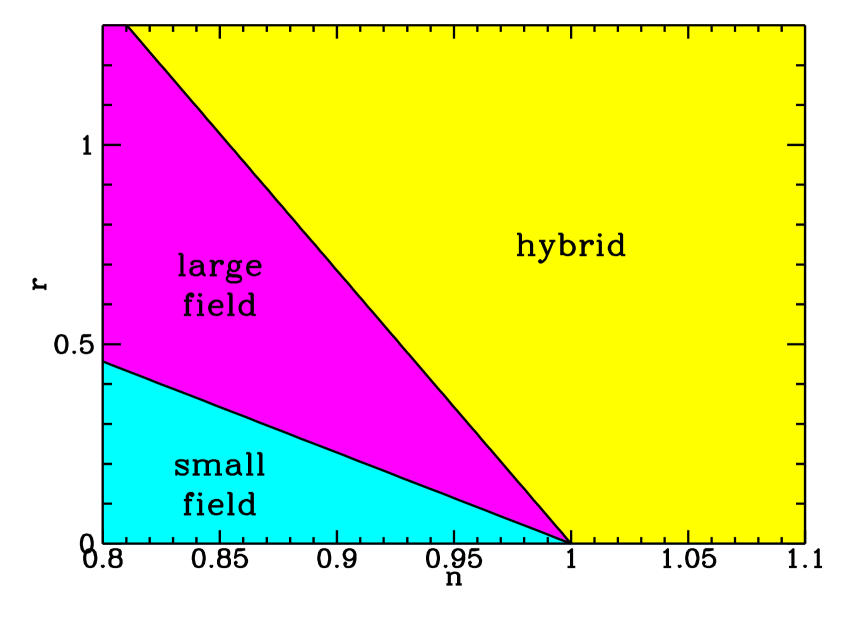
The hybrid scenario[25, 26, 27] frequently appears in models which incorporate inflation into supersymmetry. In a typical hybrid inflation model, the scalar field responsible for inflation evolves toward a minimum with nonzero vacuum energy. The end of inflation arises as a result of instability in a second field. Such models are characterized by and . We consider generic potentials for hybrid inflation of the form The field value at the end of inflation is determined by some other physics, so there is a second free parameter characterizing the models. Because of this extra freedom, hybrid models fill a broad region in the plane (Fig. 1). There is, however, no overlap in the plane between hybrid inflation and other models. The distinguishing feature of many hybrid models is a blue scalar spectral index, . This corresponds to the case . Hybrid models can also in principle have a red spectrum, .
D Linear models:
Linear models, , live on the boundary between large-field and small-field models, with and . The spectral index and tensor/scalar ratio are related as:
| (18) |
This enumeration of models is certainly not exhaustive. There are a number of single-field models that do not fit well into this scheme, for example logarithmic potentials typical of supersymmetry [18]. Another example is potentials with negative powers of the scalar field used in intermediate inflation [53] and dynamical supersymmetric inflation [32, 34]. Both of these cases require and auxilliary field to end inflation and are more properly categorized as hybrid models, but fall into the small-field region of the plane. However, the three classes categorized by the relationship between the slow-roll parameters as (large-field), (small-field, linear), and (hybrid), cover the entire plane and are in that sense complete.†††Ref. [48] incorrectly specified for large-field and for small-field. Figure 1[47] shows the plane divided up into regions representing the large field, small-field and hybrid cases.
III CMB Analysis
In this section we discuss the ability of current CMB data to place constraints on the inflationary parameter space. In particular, we wish to determine which regions of the inflationary model space are ruled out by the Boomerang and MAXIMA-1 data, and which regions are consistent with the observed data. We perform a likelihood analysis over multiple cosmological parameters and project likelihood contours onto the plane. The choice of parameters to be varied in the analysis is crucial, and different assumptions result in different constraints on the inflationary model space. In addition to and , we also vary the Hubble constant , the reionization optical depth , the amplitude of fluctuations, , (in units of ), the cold dark matter density , the vacuum energy density , and the baryon density , subject to the constraint of a flat universe , consistent with the prediction of inflation. We also assume the consistency relation (12) between and . We fix the number of neutrino species at three and we take a gaussian prior on the Hubble constant: . Note that this approach is different from many CMB parameter estimation programs, which attempt to constrain cosmological parameters in a model independent fashion. Since our object here is to falsify models, we include as many model dependent constraints as possible and examine the consistency of the data with the predictions of the models. For example, this allows us to avoid questions of parameter mis-estimation arising from features in the primordial power spectrum[54].
The Boomerang and Maxima power spectra are estimated in and bins respectively, spanning the range . In each bin, the spectrum is assigned a flat shape, . Following [55] we use the offset lognormal approximation to the likelihood . In particular we define ‡‡‡The cross-correlation between bandpowers and the offset lognormal corrections for the Boomerang and Maxima experiments are not yet public available. We tested the stability of our result including a correlation and with different lognormal distributions. We obtained near identical results with the analysis of [56] where the comparison was possible (, ).:
| (19) |
| (20) |
| (21) |
where () is the theoretical (experimental) band power, is the offset correction and is the Gaussian curvature of the likelihood matrix at the peak. Proceeding as in Refs. [57, 58], we assign a likelihood to each point in the parameter space and we find constraints on all the parameters by finding the remaining “nuisance” parameters which maximize it.
Usually there are two maximization procedures. One is based on a search algorithm through the second derivative of the likelihood matrix[57]. In this approach the ’s are computed on the way, without sampling the whole parameter space. The second approach is based on building a database of ’s on a discretized grid of the parameter space. The maxima values are then obtained from the likelihood computed on the grid[58, 59]. We adopted the database approach mainly for its robustness and the possibility to use a ’true’ marginalization method’. The bulk of our results were evaluated on a database of models sampled as follows:
| (22) | |||
| (23) | |||
| (24) | |||
| (25) | |||
| (26) | |||
| (27) | |||
| (28) | |||
| (29) | |||
| (30) |
Two parameters in particular require careful consideration: the physical baryon density and the reionization optical depth . Our constraints on the inflationary parameter space are strongly dependent on our choice of priors for . In particular, the suppressed second peak seen in the data requires either a baryon density too high to be consistent with big-bang nucleosynthesis (BBN) constraints[59], or a significant “red” tilt, , if standard BBN is assumed. For completeness, we will consider separately cases: no prior constraints on , and as suggested by the dichotomy in high and low deuterium measurements from distant quasars absorption line systems (see, e.g. Ref. [60, 61]). The second important parameter is the reionization optical depth . It is known that there is a strong degeneracy between and the tensor/scalar ratio , so that allowing for significant reionization strongly degrades the ability to distinguish tensor modes[48]. Theoretical predictions, based on the Press-Schecter formalism, show that reionization most probably occurred after redshift [62], with for flat models[63, 64]. This roughly corresponds to an optical depth [65] . Again, we consider separately 3 cases: no reionization, and .
IV Results
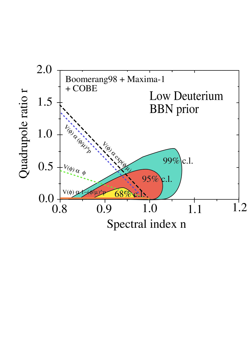
In the -plane, the parameter space is divided into regions for small-field, large-field and hybrid models as in Figure 1. Figure 2 shows the (), (), and () contours on the plane for the case of no reionization and no BBN prior. The various inflation models described in the last section and in Figure 1 are now plotted as labeled lines on the graph. (Note that the entire region to the right of the case of the exponential potential is consistent with hybrid inflation models). The lines are obtained by varying a given parameter within a class of models, e.g. for large-field models with a power-law potential what varies is the power .
The best model is nearly scale invariant, and the tensor/scalar ratio is only weakly constrained. Marginalizing over () we obtain also the constraint : (). Hybrid and small-field models are consistent with the data, but strongly tilted large-field models are in conflict with the CMB constraint to high significance. The contour on the models result in a constraint that for and for . In the power-law inflation case, , the constraint corresponds to a lower limit . The contour is marginally consistent with for and requires for in the case of a polynomial potential, and constrains in the power-law inflation case.
Figure 3 shows a similar plot when BBN constraints are included, still assuming negligible reionization. The contours in are significantly tighter than in the case with no BBN prior, and the best fit model is shifted toward tilted models: and for the low deuterium (LD) case ; and for the high deuterium (HD) case, with the scale invariant case just consistent with the data at . (Fig. 3 shows the high deuterium case.) To , large-field models are excluded entirely. The only models within are linear and small-field inflation. To , the case of a polynomial potential is constrained to for and for .
Figure 4 shows the constraints when a strong constraint on from BBN is assumed (left to right) and when the optical depth is increased. Fixing the optical depth to shifts the likelihood towards “blue” tilted models () making the scalar invariant models consistent with the data even when the BBN constraint are assumed ( for no constraint, for both BBN constraints, all at c.l.). Increasing this parameter up to moves the likelihood contours in the hybrid models region (, for LD and for HD). These models are disfavored by the dataset itself, being the best fit model at from the corresponding best fit model with . Note in particular that large-field models with tilt are strongly disfavored in all cases. Removing the consistency relation and fixing does’nt affect this conclusion and has small effect on the overall result: for no BBN constraint and we found and (marginalized over ).
V Conclusions
With the release of data from the Boomerang and MAXIMA-1 balloon flights, it is possible for the first time to place significant constraints from the cosmic microwave background on the space of possible inflation models. The data in the region , in particular, break the degeneracy between and on the first peak and produce a more stringent upper limit on for hybrid models respect to previous analysis[66, 67, 68]. In this paper we consider the observational constraints on the “zoo” of simple inflation models characterized by a single scalar field in the parameter space consisting of scalar spectral index and tensor/scalar ratio . Different classes of models make distinct predictions for the relationship between and and can in principle be differentiated by use of CMB observations. While the current data is not good enough to rule out entire classes of models, it is sufficient to place significant constraints on model parameters. Combined with constraints on the baryon density from Big-Bang nucleosynthesis, we conclude that the favored inflationary models have negligible tensor amplitude and a “red” tilt, with a best fit of and (assuming low deuterium and negligible reionization), consistent with the simplest “small-field” inflation models such as those arising from spontaneous symmetry breaking[50, 51] or from pseudo Nambu-Goldstone bosons (natural inflation[52]). Models with strong reionization favor higher values of the spectral index consistent with hybrid inflation models. Without including BBN constraints, a broad range of models are consistent with the data, including large-field and hybrid scenarios, and the favored model is nearly scale-invariant, . Future observations promise to significantly narrow the allowed regions of the parameter space, and will potentially make it possible to rule out entire classes of inflation models.
Acknowledgments
We would like to thank Edward W. Kolb, Andrei Linde, David Lyth and Jean Philippe Uzan for useful discussions. AM is grateful to Amedeo Balbi, Paolo de Bernardis, Ruth Durrer, Pedro Ferreira, Naoshi Sugiyama, Nicola Vittorio and the Boomerang Collaboration. WHK is supported in part by U.S. DOE grant DE-FG02-97ER-41029 at University of Florida.
REFERENCES
- [1] A. Guth, Phys. Rev. D 23, 347 (1981).
- [2] V. F. Mukhanov and G. V. Chibisov, JETP Lett. 33, 532 (1981).
- [3] S. W. Hawking, Phys. Lett. 115B, 295 (1982).
- [4] A. Starobinsky, Phys. Lett. 117B, 175 (1982).
- [5] A. Guth and S. Y. Pi, Phys. Rev. Lett. 49, 1110 (1982).
- [6] J. M. Bardeen, P. J. Steinhardt, and M. S. Turner, Phys. Rev. D 28, 679 (1983).
- [7] G. F. Smoot et al. Astrophys. J. 396, L1 (1992).
- [8] C. L. Bennett et al. Astrophys. J. 464, L1 (1996).
- [9] K. M. Gorski et al. Astrophys. J. 464, L11 (1996).
- [10] See, for example, N. Bahcall, J. P. Ostriker, S. Perlmutter and P. J. Steinhardt, Science 284, 1481 (1999), astro-ph/9906463.
- [11] S. Hannestad and G. Raffelt, Phys. Rev. D59, 043001 (1999), astro-ph/9805223. R. E. Lopez, S. Dodelson, A. Heckler and M. S. Turner, Phys. Rev. Lett. 82, 3952 (1999), astro-ph/9803095; R. E. Lopez, S. Dodelson, R. J. Scherrer and M. S. Turner, observations,” Phys. Rev. Lett. 81, 3075 (1998), astro-ph/9806116; W. H. Kinney and A. Riotto, Phys. Rev. Lett. 83, 3366 (1999). hep-ph/9903459; S. Hannestad, Phys. Rev. D59, 125020 (1999); astro-ph/9903475. J. Lesgourgues and S. Pastor, Phys. Rev. D60, 103521 (1999), hep-ph/9904411; J. Lesgourgues, S. Pastor and S. Prunet, asymmetry,” hep-ph/9912363; S. Hannestad, astro-ph/0005018.
- [12] P. de Bernardis et al., Nature 404, 955 (2000).
- [13] A. E. Lange et al., astro-ph/0005004.
- [14] S. Hanany et al., astro-ph/0005123.
- [15] A. Balbi et al., astro-ph/0005124.
- [16] A. Miller et al., Astrophys.J., L1-L4, 524 (1999).
- [17] P. D. Mauskopf et al., Astrophys. J. Lett. L59, 536 (2000).
- [18] For a review, see D. H. Lyth and A. Riotto, perturbation,” Phys. Rept. 314, 1 (1999), hep-ph/9807278.
- [19] J. R, Bond and Salopek, Phys. Rev. D 45, 1139, (1992), A. Linde and V. Mukhanov, Phys.Rev. D 56, 535 (1997), astro-ph/9610219.
- [20] D. Polarski and A. A. Starobinsky, Phys.Rev. D 50, 6123 (1994), astro-ph/940406; M. Kawasaki, N. Sugiyama and T. Yanagida, Phys. Rev. D 54, 2442 (1996), hep-ph/9512368.; M. Bucher, K. Moodeley, N.Turok, astro-ph/9904231; D. Langlois, A. Riazuelo, Phys. Rev. D 62, 043504, (2000).
- [21] J.A. Casas, J.M. Moreno, C. Muñoz, and M. Quirós, Nucl. Phys. B328 272 (1989); L. Kofman, A. Linde, A. Starobinsky, Phys. Rev. Lett., 76, 1011, (1996); E. Halyo, Phys. Lett. B387 43 (1996); P. Binétruy and G. Dvali, Phys. Lett. B388 241 (1996).
- [22] F. R. Bouchet, P. Peter, A Riazuelo and M Sakellariadou, astro-ph/0005022.
- [23] P. G. Ferreira, J. Magueijo, and K. M. Gorsky, Astrophys. J. Lett. 503, L1 (1998), astro-ph/9904073; J. Magueijo, Astrophys. J. Lett. 528, L57 (2000), astro-ph/9911334.
- [24] M. B. Hoffman and M. S. Turner, astro-ph/0006321.
- [25] A. Linde, Phys. Lett. B259, 38 (1991).
- [26] A. Linde, Phys. Rev. D 49, 748 (1994), astro-ph/9307002.
- [27] E. J. Copeland, A. R. Liddle, D. H. Lyth, E. D. Stewart, and D. Wands, Phys. Rev. D 49, 6410 (1994).
- [28] J. Martin and A. Rizuelo, astro-ph/0006392.
- [29] E. D. Stewart, Phys. Lett. B391, 34 (1997), hep-ph/9606241.
- [30] E. D. Stewart, Phys. Rev. D 56, 2019 (1997), hep-ph/9703232.
- [31] E. J. Copeland, I. J. Grivell, and A. R. Liddle, Report No. astro-ph/9712028.
- [32] W. H. Kinney and A. Riotto, Astropart. Phys. 10, 387 (1999), hep-ph/9704388.
- [33] L. Covi, D. H. Lyth and L. Roszkowski, Phys. Rev. D 60, 023509 (1999), hep-ph/9809310.
- [34] W. H. Kinney and A. Riotto, Phys. Lett.435B, 272 (1998), hep-ph/9802443.
- [35] L. Covi and D. H. Lyth, Phys. Rev. D 59 (1999) 063515, hep-ph/9809562.
- [36] D. H. Lyth and L. Covi, astro-ph/0002397.
- [37] A. A. Starobinski, Grav. Cosmol. 4, 88 (1998), astro-ph/9811360. D. J. Chung, E. W. Kolb, A. Riotto and I. I. Tkachev, and features in the primordial power spectrum,” hep-ph/9910437.
- [38] E. F. Bunn and M. White, Astrophys. J. 480, 6 (1997).
- [39] D. H. Lyth, Report No. hep-ph/9609431.
- [40] J. E. Lidsey, A. R. Liddle, E. W. Kolb, E. J. Copeland, T. Barriero, and M. Abney, Rev. Mod. Phys. 69, 373 (1997).
- [41] M. S. Turner, M. White and J. E. Lidsey, Phys. Rev. D 48, 4613 (1993).
- [42] D. Polarski and A. A. Starobinsky, Phys. Lett. 356B, 196 (1995).
- [43] J. García-Bellido and D. Wands, Phys. Rev. D 52, 6739 (1995).
- [44] M. Sasaki and E. D. Stewart, Prog. Theor. Phys. 95, 71 (1996).
- [45] A. A. Starobinsky, Phys. Lett. 91B, 99 (1980).
- [46] J. García-Bellido, Phys. Lett. 418B, 252 (1998).
- [47] S. Dodelson, W. H. Kinney and E. W. Kolb, Phys. Rev. D 56 3207 (1997).
- [48] W. H. Kinney, Phys. Rev. D 58, 123506 (1998).
- [49] A. D. Linde, Phys. Lett. B129, 177 (1983).
- [50] A. D. Linde, Phys. Lett. B108 389, 1982.
- [51] A. Albrecht and P. J. Steinhardt, Phys. Rev. Lett 48, 1220 (1982).
- [52] K. Freese, J. Frieman and A. Olinto, Phys. Rev. Lett. 65, 3233 (1990).
- [53] J. D. Barrow and A. R. Liddle, Phys. Rev. D 47, R5219 (1993).
- [54] W. H. Kinney, astro-ph/0005410.
- [55] J.R. Bond, A.H. Jaffe, and L. Knox, Astrophys. J. 533, 19 (2000).
- [56] A. H. Jaffe et al, Phys. Rev. Lett., Submitted, astro-ph/0007333
- [57] S. Dodelson and L. Knox, Phys. Rev. Lett. 84, 3523 (2000).
- [58] A. Melchiorri et al, Astrophys. J. Lett. L63, 536, (2000).
- [59] M. Tegmark and M. Zaldarriaga, astro-ph/0004393.
- [60] S. Burles, K. M. Nollett, J. W. Truran, and M. S. Turner, Phys. Rev. Lett. 82, 4176 (1999), astro-ph/9901157.
- [61] S. Esposito, G. Mangano, G. Miele, and O. Pisanti astro-ph/0005571.; S. Esposito, G. Mangano, A. Melchiorri, G. Miele and O. Pisanti astro-ph/0007419.
- [62] M. Tegmark and J. Silk, Astrophys. J., 420, 424, (1995).
- [63] E. A. Baltz, N.Y. Gnedin, and J. Silk, Astrophys. J. L1, 493, (1998).
- [64] Z. Haiman, 32nd COSPAR Scientific Assemby, 15-17 July, 1998, Nagoya, Japan; to appear in Adv. of Space Research.
- [65] L. M. Griffiths, D. Barbosa and A. R. Liddle, astro-ph/9812125.
- [66] A. Melchiorri, M.V. Sazhin, V. V. Shulga, N. Vittorio, Astrophys.J., 562, 518, (1999)
- [67] J.P. Zibin, D. Scott, M. White, Phys.Rev., D60, 123513, (1999)
- [68] E.V.Mikheeva, V.N.Lukash, N.A.Arkhipova, A.M.Malinovsky, Proceedings of Moriond 2000 “Energy Densities in the Universe”, Les Arcs, France, January 22-29 2000