Galaxy-dark matter correlations applied to galaxy-galaxy lensing: predictions from the semi-analytic galaxy formation models

Abstract

We use semi-analytic models of galaxy formation combined with high resolution N-body simulations to make predictions for galaxy-dark matter correlations and apply them to galaxy-galaxy lensing. We analyze cross-correlation spectra between the dark matter and different galaxy samples selected by luminosity, colour or star formation rate. We compare the predictions to the recent detection by SDSS. We show that the correlation amplitude and the mean tangential shear depend strongly on the luminosity of the sample on scales below $1\;h^{-1}{\rm Mpc}$, reflecting the correlation between the galaxy luminosity and the halo mass. The cross-correlation cannot however be used to infer the halo profile directly because different halo masses dominate on different scales and because not all galaxies are at the centres of the corresponding haloes. We compute the redshift evolution of the cross-correlation amplitude and compare it to those of galaxies and dark matter. We also compute the galaxy-dark matter correlation coefficient and show it is close to unity on scales above $r>1\;h^{-1}{\rm Mpc}$ for all considered galaxy types. This would allow one to extract the bias and the dark matter power spectrum on large scales from the galaxy and galaxy-dark matter correlations.

1 Introduction

One of the main goals of modern cosmology is to understand the processes of structure and galaxy formation in the universe. It is widely believed that large scale structure emerged from small matter density fluctuations through the gravitational instability process. Once the fluctuations became large the process of gravitational collapse led to the formation of first dark matter haloes, which subsequently merged to form larger and larger haloes. Gas initially followed the dark matter until it reached sufficiently high densities that it was able to cool efficiently and condense at the centres of the haloes. Subsequent star formation from the cold gas lead to the creation of galaxies. While the broad picture of this scenario is widely accepted its details are still poorly understood.

Observational constraints on the processes of structure and galaxy formation can be divided into three categories. In the first are observations that depend only on the distribution of the dark matter. Examples of these are velocity flows (e.g. Strauss & Willick 1995), weak lensing (e.g. Mellier 1999) or X-ray temperature function (e.g. Blanchard et al. 2000). Another example at high redshift are cosmic microwave background anisotropies (e.g. Hu et al. 2000). These direct probes of dark matter are our best hope to determine the cosmological parameters and the clustering of dark matter. In the second category are observations that only trace galaxies. Examples are galaxy luminosity function, colours, morphologies, clustering etc. These observations also depend on the underlying dark matter distribution to some extent, but the relation is often a complicated one and difficult to interpret in the absence of dynamical information. In the third category are observations that relate the properties of the galaxies to those of the dark matter. An example is the Tully-Fisher relation (Tully & Fisher 1977), which relates the luminosity of the spiral galaxies to their maximal rotational velocity, which is related to the mass of the halo in which the galaxies reside. Observations in this category are specially important in relating the process of galaxy formation to the process of structure formation. Galaxy-dark matter correlations, which can be measured through the weak lensing effects such as galaxy-galaxy lensing, galaxy foreground-background correlations or galaxy-quasar correlations, offer another example that fall into this category. The goal of this paper is to analyze these in the context of the galaxy formation models and make predictions for such observations.

Physics of galaxy formation remains a complicated and poorly understood subject and various approaches have been developed to address it. Two most commonly used approaches are hydrodynamic simulations (Blanton et al. 1999; Pearce et al. 1999) and N-body simulations coupled to the semi-analytical models (SAMs; Benson et al. 1999; Kauffmann et al. 1999; Somerville et al. 1998). First approach has the advantage of better modelling the physics, but is currently limited by the resolution. Second approach is less ab-initio and therefore may miss some important physics, but currently has a larger dynamic range. In this paper we focus on the dark matter and galaxy distribution which is quantified in terms of the cross-correlation function and the respective cross-power spectrum. Since we are particularly interested in the galactic scales which are only poorly resolved with hydrodynamic simulations we will use SAMs coupled to the N-body simulations. These are still limited in resolution and so we compare the results with analytic modelling (Seljak 2000), which under certain reasonable assumptions allows one to extend the resolution limit of the current N-body simulations.

Theoretical predictions on how galaxies trace mass, how is galaxy luminosity related to the surrounding dark matter and how can we extract these relations from the observations are essential if we are to take advantage of the large amount of data available in the near future from surveys such as Sloan Digital Sky Survey (SDSS) or 2dF. SDSS has already obtained the first detection of the galaxy-galaxy lensing with only a tiny fraction of the total data (Fischer et al. 2000). This has been based on a rough separation between the foreground and the background galaxy sample. In the future this will be done with a better precision by using the photometric redshift information, which will significantly increase the signal to noise. Photometric redshifts will also allow one to combine the signal as a function of the physical separation rather than the angular one. Larger data set will allow one to split the galaxies as a function of luminosity, colour or morphology. As we show in this paper these give quantitatively different predictions for galaxy-galaxy lensing, as well as for galaxy-quasar correlations and foreground-background galaxy correlations. This would allow one to extract the information on the environment of different types of galaxies.

The outline of the paper is as follows. In Section 2 we present the formalism, simulations and computational methods. In Section 3 we present results in terms of the cross-power spectra and respective cross-correlation functions for different galaxy samples. We also show their evolution with redshift. In Section 3.3 predictions for galaxy-galaxy lensing are given and compared with some of the existing measurements of the effect (Fischer et al. 2000). In Section 4 we consider the cross-correlation coefficient dependence on scale and galaxy type and in Section 5 we address the prospects of interpreting the cross-correlations in terms of the dark matter halo profiles. Conclusions and prospects for future work are presented in Section 6.

2 Formalism and Simulations

2.1 Cross-correlation analysis

We are interested in the distribution of the dark matter around the galaxies of a selected type, averaged over all the galaxies in the sample. We can quantify this as an excess of the dark matter density above the average as a function of the radial separation $r$. This is described by the galaxy-dark matter cross-correlation function,

$$\xi_{\rm g,dm}(r)=\left<\delta_{\rm g}(\vec{x})\delta^{*}_{\rm dm}(\vec{x}+\vec{r})\right>.$$ (1)

Here $\delta_{\rm g}$ and $\delta_{\rm dm}$ are the overdensities of galaxies and dark matter, respectively, and we used the continuous description of a random field (see Peebles 1980 and Bertschinger 1992 for a discussion of the relation between the continuous and discrete realization and interpretation of $\xi$ in terms of the excess probability). We can define similarly the galaxy correlation function $\xi_{\rm g,g}$ and dark matter correlation function $\xi_{\rm dm,dm}$ by replacing one $\delta_{\rm g}$ or $\delta_{\rm dm}$ in the above equation.

A quantity we extensively use throughout the paper is the power spectrum of the random process, which is defined as a Fourier transform of the correlation function. In the case of the cross-power spectrum we have

$$P_{\rm g,dm}(k)=\frac{1}{(2\pi)^{3}}\int\xi_{\rm g,dm}(r)e^{-i\vec{k}\cdot\vec{r}}d^{3}r,$$ (2)

where the power spectrum depends only on the module of $\vec{k}$ because of isotropy,

$$P_{\rm g,dm}(k)\delta(\vec{k}-\vec{k^{\prime}})=\left<\tilde{\delta}_{\rm g}(\vec{k})\tilde{\delta}^{*}_{\rm dm}(\vec{k^{\prime}})\right>,$$ (3)

where $\tilde{\delta}(\vec{k})$ is the Fourier transform of $\delta(\vec{x})$. Often the dark matter power spectrum is written in terms of the power contributing to the variance of the density field per logarithmic interval in Fourier space

$$\sigma^{2}(k)_{\rm g,dm}=4\pi k^{3}P_{\rm g,dm}(k).$$ (4)

2.2 Cosmological simulations and power spectrum extraction

In our work we use GIF high resolution N-body simulations carried out by the Virgo collaboration (Jenkins et al. 1998). Our analysis is constrained to the currently popular $\Lambda$CDM cosmological model with matter density $\Omega_{m}=0.3$, cosmological constant $\Omega_{\Lambda}=0.7$ and the Hubble parameter $H_{0}=70\;{\rm km\;s^{-1}Mpc^{-1}}$. The N-body simulations have $256^{3}$ particles, each of mass $1.4\cdot 10^{10}h^{-1}M_{\odot}$ in a comoving box of size $L=141h^{-1}\rm{Mpc}$. Variance of mass fluctuations on a scale of $8h^{-1}\rm{Mpc}$ was $\sigma_{8}=0.9$, in agreement with the observed abundance of clusters (Eke, Cole & Frank 1996). N-body simulations are accurate on scales above the gravitational softening scale $r_{s}=30\;h^{-1}{\rm kpc}$ and dark matter clumps with more than 10 particles were identified as haloes. For the most of the present work we apply the absolute magnitude cut to the galaxy selection which eliminates the very small haloes from the sample.

For the distribution of galaxies and their physical properties we use mock catalogues from the semi-analytic model of galaxy formation (Kauffmann et al. 1999a,b). These contain information on positions of galaxies, their absolute and apparent magnitude in several bands, star formation rate and mass contained in stars or gas. They also include the information on the halo in which they are placed, including its mass and virial radius. Empirically motivated dust correction has been applied to model the extinction for the $z=0$ sample. As shown in Kauffmann et al. 1999a,b (see also Benson et al. 1999, 2000, Somerville et al. 1998 and van den Bosch 1999) these models have been successful in reproducing a number of the observational constraints, including galaxy luminosity function, Tully-Fisher relation, pairwise velocity dispersion and galaxy correlation function.

Despite this success of the SAMs it is clear that parameterizing the complex process of galaxy formation with a few parameters is an oversimplification. It is likely that as the new data become available new parameters will need to be introduced to account for this complexity. Moreover, at present the number of predictions is small and one would like to have more independent predictions that can be verified with the new observations. Galaxy-dark matter correlations as measured through the galaxy-galaxy lensing and magnification bias provide an example of this kind. These have not been explored so far with SAMs or hydrodynamic simulations and could provide important constraints for such models.

N-body simulations together with the galaxy catalogues allow us to extract the galaxy-dark matter cross-spectra. To increase the dynamic range of the power spectrum we use the technique proposed by Jenkins et al. 1998. Instead of taking the Fourier transform of the particle distribution in a whole simulation box we divide it into $m^{3}$ cubic boxes where $m=2^{n},n=0,1,\dots,6$. We interpolate all the particles onto the small box and perform a $128^{3}$ Fourier transform. We verified that increasing the grid does not affect the resulting power spectra. This method recovers exactly all the modes periodic on scale $L/m$. Assuming these modes are statistically representative of all the modes it allows one to exploit the entire dynamic range of the simulation. To perform the FFT on a grid in the real space we use the Nearest-Grid-Point (NGP) mass assignment scheme (Hockney & Eastwood 1981), which involves the least amount of smoothing. Mass assignment however still suppresses the power and we divide each Fourier mode by a window function suitable for the NGP mass assignment (Hockney & Eastwood 1981). The averaging for a given amplitude of $k$ is taken over spherical shells in the Fourier space. For each $n$ the longest modes are sparsely sampled and it is better to use the larger box (with $n-1$) to extract those. For these reasons we only use dynamic range of 2 from one box to the next. All of the spectra are corrected for the shot noise term which is due to the discrete nature of galaxies and dark matter particles. This term is negligible for the cross-power spectrum and dark matter spectrum because of the large number of dark matter particles, except for the galaxy samples with very few galaxies in the case of cross-spectrum. However, for galaxy power spectra shot noise dominates on small scales with the amplitude inversely proportional to the number of galaxies in the sample. For rare galaxy samples such as the very bright galaxies shot noise dominates already on scales of order $1\;h^{-1}{\rm Mpc}$. This limits the accuracy of the cross-correlation coefficient extraction in such samples.

2.3 Shear and magnification derivation

Gravitational lensing of distant objects by intervening mass distribution between the source and the observer distorts the size and shape of sources as seen in the image plane. In the regime of small image distortions (weak lensing regime) observationally relevant quantities are described by the convergence $\kappa$ and the two-component shear $\vec{\gamma}=(\gamma_{1},\gamma_{2})$, which are related to the projected gravitational potential of the lens $\psi(\theta)$ via the following relations $2\kappa(\theta)=\partial_{1}\partial_{1}\psi(\theta)+\partial_{2}\partial_{2}\psi(\theta)$, $2\gamma_{1}(\theta)=\partial_{1}\partial_{1}\psi(\theta)-\partial_{2}\partial_{2}\psi(\theta)$, $\gamma_{2}(\theta)=\partial_{1}\partial_{2}\psi(\theta)$, where $\theta$ is a two-dimensional position in the lens plane. The convergence $\kappa$ and may be regarded as a projected mass density along the line of sight (ignoring photon displacement effects, see Jain, Seljak and White 1999 for justification of this assumption),

$$\kappa={3\over 2}\left(\frac{H_{0}}{c}\right)^{2}\Omega_{\rm m}\ \int_{0}^{\chi_{s}}g(\chi^{\prime},\chi_{s})\ {\delta\over a}\ d\chi^{\prime}.$$ (5)

where $g(\chi^{\prime},\chi)=r(\chi^{\prime})r(\chi-\chi^{\prime})/r(\chi)$ is the radial window function, $\chi$ is the radial distance with $\chi_{s}$ is the distance to the source galaxy, $r(\chi)$ is the angular comoving distance (equal to $\chi$ in a flat universe discussed here), $H_{0}$ is the Hubble constant, $\Omega_{\rm m}$ the matter density and $a=(1+z)^{-1}$ the expansion factor. If most of the cross-correlation signal is associated with the galaxy then we can define the comoving surface matter density $\Sigma=\int\rho d\chi$, in terms of which $\kappa=\Sigma/\Sigma_{\rm crit}$. Here $\Sigma_{\rm crit}^{-1}(\chi_{l},\chi_{s})=4\pi Gr(\chi_{l})r(\chi_{s}-\chi_{l})/ar(\chi_{s})$ is critical surface density, where $\chi_{l}$ is the comoving radial distances to the lens.

The quantity we are most interested in is tangential shear $\gamma_{t}(\theta)$ which describes elongation of images perpendicularly to the line connecting the image and the lens. It may be expressed as the 2-d shear rotated to the frame defined by the image and the lens, $\gamma_{t}(\theta)=\gamma_{1}(\theta)\cos 2\beta+\gamma_{2}(\theta)\sin 2\beta$, where $\beta$ is the relative position angle between the image and the lens. In the weak lensing regime shear is directly measurable from the image ellipticities. The relation between the mean convergence $\overline{\kappa}(\theta)$ inside a given circular aperture of radius $\theta$ and the mean tangential shear along the aperture boundary $\langle\gamma_{t}(\theta)\rangle$ is given by (Kaiser 1993, Squires & Kaiser 1996, Miralda-Escudé 1996)

$$\langle\gamma_{t}(\theta)\rangle=-\frac{1}{2}\frac{d\;\overline{\kappa}(\theta)}{d\ln\theta}.$$ (6)

Averaged projected matter density can be expressed in terms of the galaxy-dark matter cross-correlation function. Here we present both the case where the redshifts of lens galaxy and background distorted galaxy are known, as well as the case when only their distributions are. From the definition of the correlation function we have that mean number density $n(r)$ of dark matter particles at a distance $r$ from a chosen galaxy is proportional to the product of the mean number density $\bar{n}$ if they were randomly distributed in space and respective cross-correlation function. This relation may be written as

$$n(r)=\bar{n}[1+\xi_{\rm g,dm}(r)].$$ (7)

Thus at an angular separation $\theta$ from a galaxy of a given type the projected matter density is on average given by

$$\Sigma(\theta)=\int\bar{\rho}\left(1+\xi_{\rm g,dm}(r)\right)d\chi,$$ (8)

where the integration is taken along the line of sight with $\chi$ the radial distance and $\bar{\rho}$ the average matter density. Keeping $\theta$ constant requires $r^{2}=\chi_{l}^{2}+\chi^{2}-2\chi_{l}\chi\cos\theta$. We can then use $\kappa=\Sigma/\Sigma_{\rm crit}$ to determine $\overline{\kappa}$ and $\gamma_{t}$. This relation does not include the change in the focusing strength along the line of sight. A more general expression is

$$\kappa=\int_{0}^{\chi_{s}}{\bar{\rho}\over\Sigma_{\rm crit}(\chi,\chi_{s})}\left(1+\xi_{\rm g,dm}(r)\right)d\chi.$$ (9)

Except for the largest angles the dominant contribution is coming from the scales closest to the lens galaxy, in which case the approximation in equation 8 is a valid one. This simplifies the analysis, since for each pair of foreground and background galaxies we only need to compute the corresponding $\Sigma_{\rm crit}$.

When the source and lens redshifts are known (or at least can be estimated with the photometric redshift techniques) the optimal way to combine the data requires to calculate for each pair of lens and source galaxies the corresponding critical density $\Sigma_{\rm crit}(\chi_{l},\chi_{s})$ and to average over the product $\Sigma_{\rm crit}\gamma_{t}$. This can then be related directly to the integral of the correlation function in equation 8.

Often the redshifts of the sources and lenses are unknown and the signal has to be averaged over the redshift distribution of both the source and the lens galaxies. This is necessary for example when the data sample is split into the bright and faint sample (Brainerd et al. 1996, Griffiths et al. 1996, Fischer et al. 2000). The relation in this case is (Moessner & Jain 1998)

$$\kappa(\theta) = 6\pi^{2}\left(\frac{H_{0}}{c}\right)^{2}\Omega_{m}\int_{0}^{\chi_{0}}d\chi W_{1}(\chi){f(\chi)\over a(\chi)}$$ (10)

$$\times \int dkk\ P_{\rm g,dm}\left(k,\chi\right)J_{0}[kr(\chi)\theta],$$

where $W_{1}(\chi)$ is the normalized radial distribution of foreground galaxies of a given type and $f(\chi)=\int_{\chi}^{\chi_{0}}g(\chi,\chi^{\prime})W_{2}(\chi^{\prime})d\chi^{\prime}$ is the average of $g(\chi,\chi^{\prime})$ over the radial distribution of background galaxies $W_{2}(\chi^{\prime})$.

Having $\kappa(\theta)$ associated with foreground galaxies of a given type we perform an average in a circular aperture

$$\overline{\kappa}(\theta) = 6\pi^{2}\left(\frac{H_{0}}{c}\right)^{2}\Omega_{m}\int_{0}^{\chi_{0}}d\chi W_{1}(\chi){f(\chi)\over a(\chi)}$$ (11)

$$\times \int dkk\ P_{\rm g,dm}\left(k,\chi\right)\frac{2J_{1}[kr(\chi)\theta]}{kr(\chi)\theta},$$

thus we receive the mean tangential shear as a function of lens-image separation

$$\langle\gamma_{t}(\theta)\rangle = 6\pi^{2}\left(\frac{H_{0}}{c}\right)^{2}\Omega_{m}\int_{0}^{\chi_{0}}d\chi W_{1}(\chi){f(\chi)\over a(\chi)}$$ (12)

$$\times \int dkk\ P_{\rm g,dm}\left(k,\chi\right)J_{2}[kr(\chi)\theta].$$

3 Galaxy-dark matter correlations

3.1 Correlations at z=0

In this section we investigate the cross-power spectra and the cross-correlation functions for several galaxy samples. We choose galaxies of different absolute luminosity in B-band from ${\rm M}_{B}=-18$ at the completeness limit of the sample to the very rare bright galaxies with ${\rm M}_{B}<-21$. We also select red galaxies with ${\rm M}_{B}-{\rm M}_{V}>0.8$ and blue galaxies with ${\rm M}_{B}-{\rm M}_{V}<0.8$ in addition to the absolute magnitude cut.

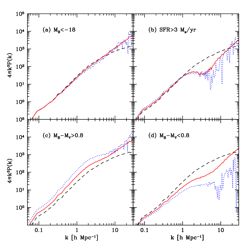
Figure 1: Power spectra of the dark matter (long dashed), galaxies (short dashed) and galaxy dark-matter cross-power spectra (solid) for selected samples of galaxies. All power spectra are at $z=0$. In panel (a) galaxy selection is $M_{B}<-18.0$, in panel (b) star formation rate $>3{\rm M}_{\odot}/{\rm yr}$, in panel (c) red colour with $M_{B}-M_{V}>0.8$ and in panel (d) blue with $M_{B}-M_{V}<0.8$, both in addition to $M_{B}<-18$.

Examples of several power spectra for redshift $z=0$ are shown in Fig. 1. In Fig. 1a we show the power spectra for galaxies brighter than ${\rm M}_{B}<-18$, for which the sample is complete in the sense that most galaxies brighter than this limit form in haloes more massive than $1.4\cdot 10^{11}h^{-1}{\rm M}_{\odot}$, which is the smallest mass halo that can form in our simulations. The galaxy power spectrum is a power law up to a large $k$, while the dark matter power spectrum is continuously changing slope and becoming less steep. The galaxies are unbiased on large scales where the two spectra agree. The cross-spectrum has a similar amplitude to the galaxy and dark matter spectrum on large scales, as expected if the galaxies are an unbiased tracer of the dark matter. Cross-spectrum grows above both galaxy and dark matter spectrum on smaller scales. This can be understood with a model where for a given halo mass range there are more individual galaxies (which contribute to the cross-spectrum) than galaxy pairs (which contribute to the galaxy spectrum, see Seljak 2000). In addition, in a smaller halo with typically just one galaxy in it the galaxy is at the halo centre with dark matter particles distributed as the halo profile. In contrast, for the dark matter particles the number of pairs at a given separation is suppressed because not all dark matter particles are at the centre. This suppresses the auto power spectrum of the dark matter relative to the cross-spectrum.

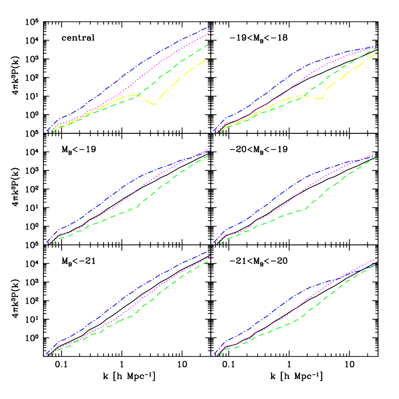
Figure 6: Halo-dark matter cross-power spectra (upper left) for mass intervals $10^{14}h^{-1}M_{\sun}<M<10^{15}h^{-1}M_{\sun}$, $10^{13}h^{-1}M_{\sun}<M<10^{14}h^{-1}M_{\sun}$, $10^{12}h^{-1}M_{\sun}<M<10^{13}h^{-1}M_{\sun}$ and $10^{11}h^{-1}M_{\sun}<M<10^{12}h^{-1}M_{\sun}$, from top to bottom. Other plots show the galaxy-dark matter cross-power spectra for different galaxy samples as a function of halo mass (similarly to upper left panel) and for all galaxies within that sample (solid). In the bottom four plots the interval with $10^{11}h^{-1}M_{\sun}<M<10^{12}h^{-1}M_{\sun}$ interval is not shown because there are few or no galaxies within the sample in such low mass objects.

In Fig. 1a the transition between the large and small scales in the cross-spectrum is continuous for the sample selected only by absolute magnitude. Figure 1b shows the same for the star-forming galaxies. These are mostly in the field and show a more prominent transition in the cross-spectrum between the correlations between haloes for $k<3\;h{\rm Mpc}^{-1}$ and the profile of the haloes themselves at $k>3\;h{\rm Mpc}^{-1}$. For galaxies selected only by magnitude groups and clusters also contribute to correlations, which fills in the transition region between the two (see also fig. 6 in Seljak 2000), while for star forming galaxies which are predominantly in the field groups and clusters do not contribute.

In Fig. 1c,d red and blue samples of the galaxies are shown. Red galaxies are quite biased on large scales, indicating that they form predominantly in haloes more massive than the nonlinear mass scale (i.e. groups and clusters). On smaller scales the cross-correlation drops off more rapidly than the corresponding spectra in Fig. 1a and b. This is because red galaxies in this model typically do not reside at the halo centres and thus the power spectrum suffers similar suppression as the dark matter. In contrast, blue galaxies in Fig. 1d are unbiased on large scales. The galaxy power spectrum is flat on small scales indicating there are very few haloes with more than one blue galaxy. Cross-spectrum shows similar features on large scales, but begins to rise on small scales where the galaxies that are at the halo centres become dominant and the cross-spectrum reflects their own dark matter halo profiles. Overall, the blue galaxies show similar features to the star forming galaxies, although the latter show more prominent transition between intra and inter halo correlations.

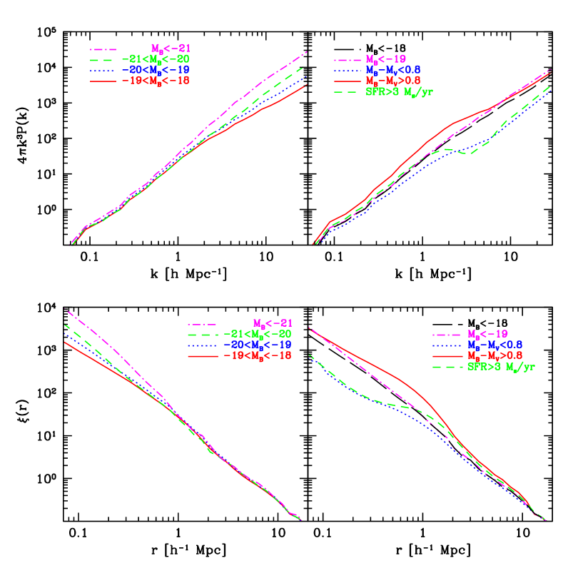
Figure 2: Galaxy-dark matter cross-power spectra and respective cross-correlation functions for luminosity bands (left panel) and colour and star formation rate (right panel). In the lower panels the cross-correlation functions are presented for the same samples as in the upper panel.

Fig. 2 shows the cross-spectra and the cross-correlation functions for galaxies in narrow magnitude bands in addition to the galaxies in Fig. 1. On large scales the spectra of narrow-band magnitude galaxies agree, indicating that the galaxies on average reside in unbiased haloes around or somewhat below the nonlinear mass. Significant fraction of them reside in groups and clusters, which explains the smooth transition between the large and the small scales. On small scales however there are significant differences in the amplitude of correlations, which increases with the brightness of the sample. This is similar to the Tully-Fisher relation, where the luminosity of spiral galaxies is correlated with the maximal circular velocity of the disc, which is correlated with the circular velocity of the halo in the SAMs used here. The differences between the models are significant already at $100\;h^{-1}{\rm kpc}$, where the complications because of the baryonic effects on the dark matter distribution are negligible. This shows the potential of galaxy-galaxy lensing, which can provide independent information on the relation between the galaxy luminosity and its dark matter environment and can probe regions where baryon effects are negligible. Because of the weakness of the signal this can only be done statistically for a large sample of the galaxies and one must understand the complications caused by effects such as the contribution from groups and clusters, number of galaxies inside the halo as a function of halo mass, central versus satellite galaxies inside the halo etc. These are discussed further below.

3.2 Redshift evolution of cross-correlation

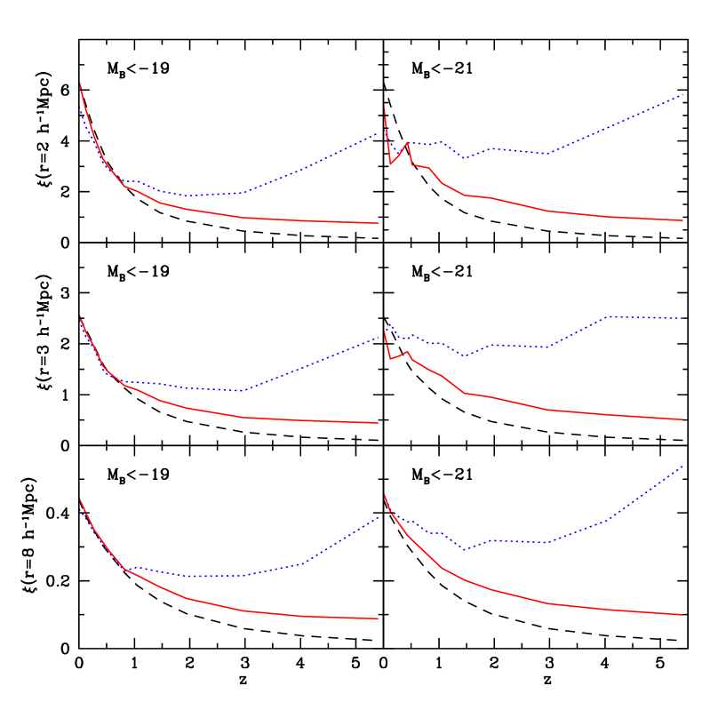
Figure 3: Evolution of the cross-correlation function for two galaxy samples, $M_{B}<-19$ (left panel) and $M_{B}<-21$ (right panel), at separation $2\;h^{-1}{\rm Mpc}$, $3\;h^{-1}{\rm Mpc}$ and $8\;h^{-1}{\rm Mpc}$. Solid line shows galaxy-dark matter cross-correlation amplitude, dotted galaxy auto-correlation and dashed the dark matter auto-correlation.

From the high z catalogs of the galaxy and dark matter positions we extract the evolution of the galaxy-dark matter correlation function for galaxies brighter than ${\rm M}_{B}<-19.5$ and brighter than ${\rm M}_{B}<-21$. No dust correction has been applied to these data so we focus only on the amplitude of the correlation function at different scales as a function of redshift. Figure 3 shows the redshift evolution of the amplitude of the correlation function at $2\;h^{-1}{\rm Mpc}$, $3\;h^{-1}{\rm Mpc}$ and $8\;h^{-1}{\rm Mpc}$ for all three spectra. The amplitude of the dark matter correlation function decreases with redshift because of gravitational instability, which causes density perturbations to grow in time. On the other hand, the amplitude of the galaxy correlation function first decreases for the same reason, but then increases again because at higher redshifts bright galaxies are only found in the rare massive haloes, which are biased with respect to the dark matter (Kauffmann et al. 1999b). For brighter galaxies (right panels) the biasing at higher redshift is more important and leads to a larger amplitude than for fainter galaxies. Amplitude of the cross-correlation function falls in-between the amplitudes of dark matter and galaxy correlation function. From the model with correlation coefficient of unity discussed below one predicts it to be the geometric mean, which is a good description even for the galaxies that are highly biased, since we are looking at scales above $1\;h^{-1}{\rm Mpc}$, where correlation coefficient is close to unity (see next section). The cross-correlation amplitude typically does not increase at higher z, but becomes flat.

3.3 Galaxy-galaxy lensing predictions

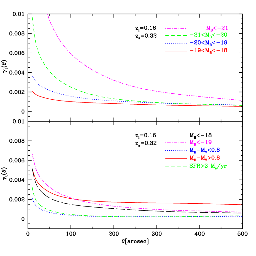
Figure 4: Tangential shear as a function of angular distance from the lens galaxy for the same models as in figure 2. Background galaxies are assumed to be placed at a fixed redshift $z_{s}=0.32$ and foreground galaxies at a redshift $z_{l}=0.16$ that mimics the mean redshift of lenses and sources for SDSS galaxy-galaxy lensing detection.

In this subsection we present predictions of galaxy-galaxy lensing effect for samples of galaxies discussed in previous section. For simplicity we model source and lens galaxies as being at fixed redshifts $z_{l}=0.16$ and $z_{s}=0.32$, so that the critical surface density corresponds to that of SDSS sample (Fischer et al. 2000). We use $z=0$ dust corrected sample to extract the galaxy-galaxy lensing signal, but we verified that for a shallow surveys such as the SDSS this assumption does not significantly affect the results. Results presented in Fig. 4 give the mean tangential shear as a function of the observed angular separation from the lens. For the considered cosmological model $10\;{\rm arcsec}$ corresponds to a physical distance in the lens plane of $22.4\;h^{-1}{\rm kpc}$. At the redshift $z=0.16$ galaxy of absolute luminosity ${\rm M}_{B}=-20$ corresponds to an apparent magnitude ${\rm m}_{B}=19.4$.

Plots in the upper panel of Fig. 4 are for the same luminosity intervals as in Fig. 2. For the bright galaxies tangential shear is larger than for the faint ones as predicted from the results in Fig. 2. Note also that the slope increases with luminosity. Fitting the spectra to a power law gives the slopes varying from $-0.26$ at the faint end to $-0.54$ at the bright end, but in general single power law provides a poor fit to the spectra (the slope steepens at larger angles). The slope is considerably shallower than the singular isothermal sphere (SIS) distribution with the slope $-1$, predicting that with better data one should be able to see the deviations from SIS. To compare it to the Tully-Fisher relation one can compare the predictions for $\gamma_{t}$ at a given angle, which we choose to be $\theta=100\;{\rm arcsec}$ to maximize the signal to noise in SDSS. This corresponds to $220\;h^{-1}{\rm kpc}$ transverse distance from the galaxy. Assuming $\gamma_{t}\propto v_{c}^{2}$ where $v_{c}$ is the circular velocity and fitting this to the relation $L\propto v_{c}^{\alpha}$ one finds $\alpha=3.5$, which is in a good agreement with the Tully-Fisher relation. This agreement is however partially fortuitous, because the slope of $\gamma_{t}$ is not well fit with the SIS model and so the $L-v_{c}$ relation must change with the angle at which the comparison is made.

In the lower part of Fig. 4 we show the results for ${\rm M}_{B}<-18$, ${\rm M}_{B}<-19$, star forming galaxies, red and blue galaxies. Since the luminosity function peaks at ${\rm M}_{B}=-19$ galaxies brighter than ${\rm M}_{B}<-18$ to ${\rm M}_{B}<-19$ should be compared to the SDSS apparent magnitude selected sample. It is encouraging that the predictions are in a good agreement with the observed signal. We should caution that this is not meant to be a quantitative analysis of SDSS results, because we do not simulate SDSS colour bands, selection criteria and galaxy redshift distribution, all of which depend also on the luminosity function of the sample and not just on the relation between galaxy luminosity and its dark matter halo environment. With photometric redshift information the dependence on the luminosity function can be eliminated and observations will provide a more direct constraint on the dynamical environment of the galaxies.

In Fig. 5 we show mean tangential shear dependence on the angular scale for red, blue and star forming galaxies, all with the luminosity cut ${\rm M}_{B}<-18$. Also shear for all galaxies brighter than ${\rm M}_{B}=-18$ is shown. Squares in this figure are observational points from SDSS (Fischer et al. 2000). Here we include the evolution of the cross-correlation function with redshift. Realistic lens and source distributions provided by the SDSS team are used in equation (12). They were derived as approximation of the respective SDSS distributions by the power-law with exponential cut-off of the form

$$W_{i}(z)=\frac{\beta_{i}z^{2}}{(z_{i})^{3}\Gamma\left(3/\beta_{i}\right)}e^{-\left(\frac{z}{z_{i}}\right)^{\beta_{i}}}$$ (13)

with $z_{1}=0.17$, $\beta_{1}=2.3$ and $z_{2}=0.35$, $\beta_{2}=1.7$ for lens and source samples respectively.

Our galaxy samples are roughly complete for galaxies brighter than ${\rm M}_{B}=-18$ so we miss some lensing signal from the nearby galaxies ($z<0.02$) when we use SDSS window functions $W_{1}(\chi)$ and $W_{2}(\chi)$. But uncertainties related to measured source redshift distribution are likely to be more important in this comparison.

Qualitatively the predictions follow the observations, but we notice that predicted lensing signal is above that detected by SDSS specially on large scales. One of the reasons for this behaviour is the discrepancy between the luminosity function from simulations we base on (Kauffmann et al. 1999a) and that obtained from observations (Lin et al. 1997). Modelled luminosity function in the $\Lambda CDM$ model lacks less luminous galaxies, fainter than ${\rm M}_{B}=-21$, and has an excess of very luminous galaxies, brighter than ${\rm M}_{B}=-23$, when compared to the present day observations. Since as shown in Fig. 2 there is a strong luminosity bias expected for the cross-correlation amplitude this enhances the theoretical prediction for the shear amplitude. The other uncertainty is already mentioned poorly known redshift distribution function. Both of these currently limit the interpretation of results, but will be eliminated once the photometric redshift techniques become realiable. This is specially promising in the case of SDSS where 5 colour photometry should enable one a very accurate redshift determination.

4 Cross-correlation coefficient

If the bias between the galaxies and the dark matter is not constant, as indicated from the results in Fig. 1, then one cannot use its determination at a given scale and apply it at another scale. This complicates the extraction of the dark matter power spectrum from the galaxy power spectrum and additional information is necessary to break the degeneracy. One can parameterize the ignorance with a scale dependent bias (van Waerbeke 1998, Dolag & Bartelmann 1998), where the relation between the galaxy, cross and matter power spectra is $P_{\rm g,dm}(k)=b(k)P_{\rm dm,dm}(k)$ and $P_{\rm g,g}(k)=b^{2}(k)P_{\rm dm,dm}(k)$. In this case from a measurement of galaxy and cross-spectrum one can determine both $b(k)$ and $P_{\rm dm,dm}(k)$. Even this relation is however not general, since the bias factor that relates one pair of spectra may not be the same as that for another pair. One can generalize this by introducing the cross-correlation coefficient between the galaxy and the dark matter power spectrum

$$r^{2}(k)=\frac{P_{\rm g,dm}^{2}(k)}{P_{\rm g,g}(k)P_{\rm dm,dm}(k)}.$$ (14)

This definition implies that in the case of a scale dependent but linear bias discussed above the cross-correlation coefficient $|r(k)|=1$.

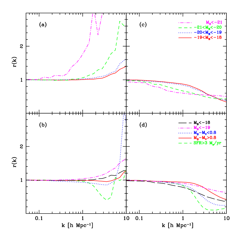
Figure 8: Correlation coefficient $r(k)$ as a function of wavevector $k$ and galaxy sample. In panels (a) and (b) $r(k)$ is derived from the shot noise corrected spectra, while in panels (c) and (d) without the shot noise correction. Galaxy samples are the same as in the Fig. 2.

In Fig. 8 we present the correlation coefficient as a function of scale for a set of galaxy samples selected by luminosity, colour or star formation rate criteria. In the right panels we show the correlation coefficient without the subtraction of the shot noise term arising form the discreteness of galaxies. In this case the correlation coefficient is constrained to $|r(k)|\leq 1$. More commonly however the shot noise is subtracted from the galaxy spectrum, which is shown in the left panels of Fig. 8. In this case for all of the considered galaxy samples the correlation coefficient remains close to unity up to $k\sim 1\;h{\rm Mpc}^{-1}$. This is encouraging because when $r(k)=1$ one can extract the bias parameter $b(k)$ and the dark matter power spectrum $P_{\rm dm,dm}(k)$ directly by measuring the galaxy power spectrum and the cross-power spectrum from the galaxy-galaxy lensing. This means that at least on large scales there is hope that bias could be determined with this method.

The correlation coefficient remains closer to unity on small scales when the shot noise is subtracted as opposed to when it is not. This is related to the fact that for a given halo mass the pair weighted number of galaxies inside the halo $\langle N(N-1)\rangle^{1/2}$ agrees with the linearly weighted number $\langle N\rangle$ for large halo masses (Seljak 2000) and that for large haloes there are many galaxies inside the halo so the central galaxy, if present, does not have a dominant contribution. Since the power spectrum on large (but still nonlinear) scales is dominated by large haloes this gives $r(k)\sim 1$. For small haloes typically $\langle N\rangle>\langle N(N-1)\rangle^{1/2}$ because there are many haloes with just one galaxy in it, which gives rise to $r(k)>1$ when shot noise is subtracted from the galaxy spectrum. In addition, for haloes with just one galaxy this galaxy is usually at the centre of the halo, which enhances the cross-correlation relative to the case where the galaxies are distributed like dark matter inside the halo (the distinction between the central galaxy and all galaxy cross-correlation is discussed further in the next section). Both of these effects become prominent when $\langle N\rangle<1$ and so are more important for galaxies that are rarer and/or on smaller scales where small haloes dominate. This agrees with the results in Fig. 8, where for the brightest and rarest sample of galaxies, ${\rm M}_{B}<-21$, the correlation coefficient increases monotonically already from $k\sim 0.5\;h{\rm Mpc}^{-1}$, whereas for the faintest and most abundant sample ${\rm M}_{B}<-18$ the cross-correlation coefficient is unity up to $k\sim 3\;h{\rm Mpc}^{-1}$.

It is interesting to note that for the sample of red galaxies (${\rm M}_{B}-{\rm M}_{V}>0.8$ and ${\rm M}_{B}<-18$), which exhibit a strong scale dependent bias as seen from Fig. 1, $r(k)$ is unity over several orders of magnitude in $k$. In small haloes where $\langle N\rangle\ll 1$ one has $\langle N\rangle\sim\langle N(N-1)\rangle^{1/2}$ (Seljak 2000). These galaxies therefore cannot be the central galaxies inside the haloes which would give $\langle N\rangle>\langle N(N-1)\rangle^{1/2}$. For the same reason the cross-spectrum is also not enhanced relative to the dark matter, both of which explains why $r(k)\sim 1$ over the entire range of scales. While this is suggestive we should be cautious not to overinterpret these results since SAMs may not be accurate in such detailed properties. It will be interesting to examine whether this prediction can be confirmed from the observations directly.

For galaxies with star formation rate (SFR) above $3{\rm M}_{\odot}/{\rm yr}$ the cross-correlation coefficient $r(k)$ has a strong decrease on scales of order $2-4\;h{\rm Mpc}^{-1}$. This is caused by a decrease in $P_{\rm g,dm}(k)$ (and $P_{\rm g,g}(k)$) relative to $P_{\rm dm,dm}(k)$. The reason for this decrease is the transition from the correlations between the haloes to correlations inside the halo, which is prominent for star forming galaxies which are predominantly in the field, but is washed out by the group and cluster contribution in the dark matter power spectrum.

5 Dark matter halo profiles

In previous sections we have presented the predictions for the galaxy-dark matter cross-correlations for various galaxy selections. We have shown that the predictions strongly depend on the galaxy luminosity, colour and star forming rate. For example, we observe a strong luminosity dependence with more luminous galaxies showing a stronger cross-correlation on small scales because such galaxies reside in more massive haloes. These haloes are still below the nonlinear mass scale and no luminosity bias caused by halo bias is observed on large scales, nor is any luminosity bias observed for galaxy auto-correlation. This shows that galaxy-galaxy lensing can be a sensitive probe of halo masses for different galaxy types. Such interpretation was the basis for most of the galaxy-galaxy lensing analysis so far (Brainerd et al. 1996, Griffiths et al. 1996 , Hudson et al. 1998). Still, the relation between the cross-correlation spectrum and the halo mass profile may be a complicated one and in this section we explore this in more detail.

In the hierarchical clustering picture galaxies form in the dark matter haloes which subsequently merge into larger structures. Galaxies which are not members of a cluster or a group at the time of observation should have more extended haloes than those of same luminosity already swollen by a cluster because tidal forces in a potential well of a cluster tend to strip the galaxies of their haloes. Present observations of the weak gravitational lensing within the clusters seem to support this picture (Natarajan et al. 1999). However, such galaxies are nevertheless embedded in larger haloes and galaxy-galaxy lensing will be sensitive also to the gravitational lensing effect of these more massive and more extended structures. This effect is specially important on scales above $100\;h^{-1}{\rm kpc}$ where the haloes of individual galaxies have only a weak signal which can easily be dominated by a sub-population of galaxies in groups and clusters (Seljak 2000). This effect is also important on smaller scales, because there is a range of halo masses that contribute to galaxies selected by their (absolute or apparent) luminosity and haloes of different mass can dominate on different scales. This makes the interpretation of the cross-correlation in term of the halo profile more complicated than simply an averaged dark matter profile of a typical galaxy.

Plots in Fig. 6 show the cross-power spectra for several galaxy types selected by their intrinsic luminosity as a function of halo mass. Smaller haloes give lower amplitude of the cross-power spectrum as expected. Note that for most galaxy types the total cross-spectrum shown with a dotted line does not agree with any individual mass range. The logarithmic slope $\alpha(k)=d\ln\sigma^{2}(k)/d\ln k$ of the total cross-spectrum is shallower that the slope of individual mass intervals (Fig. 7). On larger scales the cross-spectrum is dominated by the high mass range of the haloes, while on smaller scales smaller haloes become dominant and since these give lower amplitude of the cross-spectrum the overall slope is shallower. The only exception are the very bright galaxies with $M_{B}<-21$ which seem to reside predominantly in haloes more massive than $10^{13}h^{-1}M_{\sun}<M<10^{14}h^{-1}M_{\sun}$ and their cross-correlation function agrees well with the cross-correlation for this mass interval.

Second complication which is important for large haloes such as groups and clusters is that when there are many galaxies inside the halo most of them are not at the halo centre. When a galaxy is at the outskirts of a halo the lensing effect will on average be reduced. If the galaxies are distributed like the dark matter then one can account for this effect. However, galaxies may not be distributed in the same way as the dark matter inside the haloes (Diaferio et al. 1999) and this becomes difficult to model analytically. This effect is shown by comparing the first plot of Fig. 6, where the cross-spectra of central galaxies are shown as a function of halo mass intervals, to the other plots in that figure, where all the galaxies inside the halo are selected. For the two most massive intervals there is a significant difference between the central galaxy and all galaxies cross-spectra. The all galaxy spectra are substantially lower in amplitude as expected if most galaxies are not central. For lower mass intervals the difference between the two is smaller, since such haloes contain on average at most one bright galaxy, which is usually the central one.

It is instructive to investigate the slope of the cross-spectrum. For central galaxies this gives the slope of the dark matter profile as a function of scale. On small scales the slope approaches $\alpha\sim-1.5$ for the largest haloes with mass range $10^{14}h^{-1}M_{\sun}<M<10^{15}h^{-1}M_{\sun}$ for which the force resolution in units of virial radius is the highest. It is possible that the slope would become even shallower if higher resolution simulation are used, although some of such higher resolution simulations suggest the slope remains close to $\alpha\sim-1.5$ down to very small scales (Moore et al. 1999). This slope steepens to $\alpha\sim-2.5$ at the virial radius, beyond which the contribution from the other haloes becomes important and makes the slope less steep again. The behaviour for smaller halo mass intervals is similar, but shifted to smaller scales. At the resolution limit ($k\sim 20\;h{\rm Mpc}^{-1}$) the slope decreases with the decreasing halo mass, caused by the finite force resolution. For the lowest mass interval the transition between the halo profile and other halo correlations is quite prominent, but this is at least in part caused by the finite mass resolution because there are no very small haloes very close to the virial radius of such haloes. For all the galaxies, except the very brightest ones, the cross-spectrum slope is always shallower than for the central galaxies when viewed as a function of the halo mass.

6 Conclusions

We have investigated the galaxy-dark matter cross-correlation function and power spectrum using the semi-analytic galaxy formation models coupled with a high resolution N-body simulation. These cross-correlation spectra are the necessary ingredients to interpret the observed correlations based on weak lensing and galaxy positions. Examples are galaxy-galaxy lensing, QSO-galaxy correlations and foreground-background galaxy correlations. The advantage of the approach used here is that it includes many complicating effects such as the variety of the dark matter environments around the galaxies, the distribution of galaxies inside the dark matter haloes, correlations between the galaxies and the dark matter in the neighbouring haloes. The limitation of this approach is the mass and force resolution, which limits our study to haloes more massive than $10^{11}h^{-1}M_{\sun}$ (limiting the completeness of galaxy sample to $M_{B}<-18$) and scales larger than $50\;h^{-1}{\rm kpc}$ . This can be overcome to some extent by using the analytic model, which can extend these results to smaller scales (Seljak 2000).

The cross-correlation spectra on large scales fall between the dark matter and galaxy auto-correlation spectra. As a function of redshift the correlation strength of bright galaxies first decreases to $z\sim 1$ and then remains approximately flat because such galaxies become rare and biasing increases above unity, even if the dark matter correlation strength continues to decrease. In terms of the cross-correlation coefficient we find it is close to unity on large scales. This is good news for attempts to determine the scale dependent bias and the dark matter power spectrum directly from the galaxy correlations and the galaxy-galaxy lensing. It breaks down on small scales where effects such as the average number of galaxies inside the halo dropping below unity and presence of central galaxies cause the cross-correlation spectrum to exceed the auto-correlation spectra. This happens on larger scales for rarer galaxies, which are therefore less suitable for the determination of the dark matter power spectrum.

While on large scales the cross-correlations reflect clustering of large scale structure, on small scales they reflect more the dark matter environments around galaxies. These have been often interpreted as the dark matter profiles of haloes, but such interpretation is complicated by the effects of multiple galaxies inside clusters and by having different halo mases dominate on different scales. For example, the observed signal at $1\;h^{-1}{\rm Mpc}$ by SDSS (Fischer et al. 2000) does not mean that the haloes of galaxies such as our own can be observed at such large distances, but rather that groups and clusters extend to these distances or that haloes are correlated with neighbouring haloes. Still, the predicted signal on small scales does increase with the galaxy luminosity, as predicted by the Tully-Fisher relation if the dark matter makes a significant contribution to the maximal rotation velocity. This shows that the cross-correlations can become a complementary tool to study the dark matter environments of the galaxies. This can be potentially a powerful probe of the dark matter around the galaxies, because it is sensitive to larger distances from the centre which are less affected by the baryonic component. The upcoming surveys such as SDSS and 2dF should be able to extract this information with a high statistical precision, making galaxy-galaxy lensing an important observational tool in connecting galaxies to their dark matter environment.

Figure 5: Tangential shear as a function of angular distance. Background and foreground galaxies are assumed to be distributed as in the SDSS galaxy-galaxy lensing observations. SDSS detection in the $r^{\prime}\rm{-band}$ is presented as squares in the upper panel.

Figure 7: The slope of the cross-power spectra shown in Fig. 6. The line types are the same as in Fig. 6.

References

- [1] Benson A.J., Cole S., Frenk C.S., C.M.Baugh, Lacey C.G., 2000, MNRAS, 311, 793
- [Benson 2000] Benson A.J., Pearce F.R., Frenk C.S., C.M.Baugh, Jenkins A., astro-ph/9912220
- [2] Bertschinger E., 1992, the Universe, Proc. UIMP Summer School, ed. V.J.Martinez, M.Portilla, D.Saez
- [3] Blanchard A., Sadat, R., Bartlett J. G. & Le Dour, M., astro-ph/9908037
- [4] Blanton M., Cen R., Ostriker J.P., Strauss M.A., 1999, ApJ, 522, 590
- [] Brainerd T.G., Blandford R.D., Smail I., 1996, ApJ, 466, 623
- [] Dolag K., Bertelmann M., 1997, MNRAS, 291, 446
- [] Diaferio A., Kauffmann G., Colberg J.M. & White S.D.M., 1999, MNRAS, 307, 537
- [] Eke V.R., Cole S., Frank C.S., 1996, MNRAS, 282, 263
- [] Fischer P., et al., 2000, astro-ph/9912119
- [5] Griffiths R. E., Casertano S., Im M., Ratnatunga K. U., 1996, MNRAS, 282, 1159
- [Hockney & Eastwood 1981] Hockney R.W., Eastwood J.W., Computer Simulation Using Particles, McGraw-Hill, 1980
- [6] Hu, W., Fukugita, M., Zaldarriaga M., & Tegmark, M. 2000, astro-ph/0006436
- [7] Hudson M.J., Gwyn S.D.J., Dahle H., Kaiser N., 1998, ApJ, 503, 531
- [Jain et.al. 1995] Jain B., Mo H.J. & White S.D.M., 1995, MNRAS, 276, L25
- [] Jain B., Seljak U., White S.D.M., 2000, ApJ, 530, 547
- [Jenkins et.al. 1998] Jenkins A., Frenk C.S., Pearce F.R., Thomas P.A., Colberg J.M., White S.D.M., Couchman H.M.P., Peacock J.A., Efstathiou G., Nelson A.H., 1998, ApJ, 499, 20
- [Kaiser & Squires 1993] Kaiser N., Squires G., 1993, ApJ, 404, 441
- [Kauffmann et.al 1999] Kauffmann G., Colberg J.M., Diaferio A. & White S.D.M., 1999, MNRAS, 303, 188
- [] Kauffmann G., Colberg J.M., Diaferio A. & White S.D.M., 1999, MNRAS, 307, 529
- [8] Lin H., Kirshner R., Schechtman S.A., Landy S.D., Oemler A., Tucker D.L., Schechter P.L., 1997, ApJ, 464, 60
- [] Mellier Y., 1999, ARA&A, 37, 127
- [] Miralda-Escudé J., 1996, in Proc. IAU Symposium no.173, ed. C.S.Kochanek, J.N.Hewitt, Kluwer
- [Mo & White 1996] Mo H.J., White S.D.M., 1996, MNRAS, 282, 347
- [9] Moessner R., Jain B., 1998, MNRAS, 294, L18
- [10] Moore B., Quinn T., Governato F., Stadel J., Lake G., 1999, MNRAS, 310, 1147
- [] Natarajan P., Kneib J.P., Smail I., 1999, astro-ph/9909349
- [11] Pearce F.R., Jenkins A., Frenk C.S., Colberg J.M., White S.D.M., Thomas P.A., Couchman H.M.P., Peacock J.A., Efstathiou G., 1999, ApJ, 521, L99
- [Peebles 1980] Peebles P.J.E., 1980, The Large Scale Structure of the Universe, Princeton Univ. Press, Princeton, NJ
- [] Schneider P., Ehlers J., Falco E., 1992, Gravitational Lenses, Springer
- [Seljak 2000] Seljak U., 2000, astro-ph/0001493
- [12] Somerville R.S., Lemson G., Kolatt T.S., Dekel A., astro-ph/9807277
- [] Squires G., Kaiser N., 1996, ApJ, 473, 65
- [] Strauss M.A., Willick J.A., 1995, Phys.Rep., 261, 271
- [13] Tully R.B., Fisher J.R., 1977, ApJ, 54, 661
- [14] Van den Bosch F. C., 2000, ApJ, 530, 177
- [] Van Waerbeke L., 1998, A&A, 334, 1