The GHz-Peaked Spectrum radio galaxy 2021+614: Detection of slow motion in a compact symmetric object

Abstract

We have analysed VSOP (VLBI Space Observatory Programme) data at 5 GHz and ground-based VLBI (Very Long Baseline Interferometry) data at 15 GHz for the GHz-Peaked Spectrum (GPS) radio galaxy 2021+614. Its morphology is consistent with it being a compact symmetric source extending over $30\,h^{-1}$ pc. From a comparison with earlier observations we have detected an increase in the separation and a decrease in the size of the two most prominent components. We determine the projected speed with which these two components recede from each other to be $0.12\pm 0.02\,h^{-1}\,c$. Given the projected separation of the two components of $16.1\,h^{-1}$ pc, the infered kinematic age is $440\pm 80$ years, measured in the source reference frame. These results provide additional support for the contention that compact symmetric radio objects are young and the precursors of the classical FR I or FR II radio sources. The sizes of individual components appear to contract with time which is not consistent with the self-similar evolution model for peaked spectrum sources.
In order to overcome problems related to the estimation of uncertainties for separation measurements between source components, we have developed and applied a method that compares two uv-data sets obtained at different epochs. This method parametrizes the most important structural change, the increase in separation between components, by rescaling the u and v axis of the amplitude interference pattern. It provides best-fit values for the parameters and uses a bootstrap method to estimate the errors in the parameters.

1 Introduction

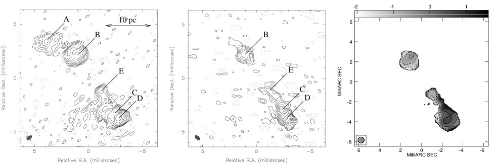
Figure 1: 5 GHz VSOP image (left) and 15 GHz global VLBI image (middle). The rms noise is 0.5 mJy/beam for the 5 GHz image and 0.9 mJy/beam for the 15 GHz image. Image peaks are 0.475 Jy/beam and 1.12 Jy/beam, respectively. Contour levels are drawn at -2, 2, 4, 8, 16, …, 512, (1024) $\times$ the respective rms noise. The restoring beams are $0.56\times 0.27$ mas, $-50.3\degr$ and $0.56\times 0.30$ mas, $47.4\degr$, respectively. At $z=0.2266$, 1 mas corresponds to $2.30\,h^{-1}$ pc. (Right) Image of the 5 – 15 GHz spectral-index, $\alpha$ ($S_{\nu}\propto\nu^{\alpha}$). The spectral index was calculated in regions with intensity higher than 5-$\sigma$ in both images. Contour levels are drawn at spectral index values of -1.5, -1.0, -0.5, 0.0, 0.5 and 1.0; negative levels and the zero level are dashed. The restoring beam is 0.6 mas circular.

Despite many years of study of extragalactic radio sources, it is still unclear how they are formed and evolve. A crucial element in the study of their early evolutionary stages is to identify the young counterparts of old and extended FR I/FR II objects. Good candidates for young radio sources are those with peaked spectra, GHz-Peaked Spectrum (GPS) sources and Compact Steep-Spectrum (CSS) sources, because they are small in angular size as expected for young sources. GPS sources are characterized by a simple convex radio spectrum peaking at a frequency of about 1 GHz and are typically 100 pc in size. CSS sources have peaks in their spectra at lower frequencies and have projected linear sizes of $<15$ kpc.
The best direct evidence for very low kinematic ages has now been found for a few GPS radio galaxies. Measurements of hotspot advance speeds, from which an age estimate can be made, have been obtained for 0108+388 (Owsianik et al. Owsianik2 (1998)), 0710+439, 2352+495 (Owsianik & Conway Owsianik1 (1998); Owsianik et al. Owsianik3 (1999)) and 1943+456 (Polatidis Polatidis (1999)). The hotspot advance speeds are typically of order $0.1\,h^{-1}\,c$, translating into ages of a few hundred to a few thousand years. All these sources belong to the morphological class of Compact Symmetric Objects (CSO), which are characterized by their small size ($<500$ pc) and symmetric radio morphology.
Having established that CSOs are young it is interesting to examine them at a number of points along their evolutionary track in the $P$–$D$ (luminosity – linear size) diagram, and to carry out investigations at several radio wavelengths with a range of angular resolution and limiting flux density. We are investigating a sample of 11 bright GPS sources at 5 GHz with VSOP. These observations have been complemented by VLBI observations at 15 GHz to obtain matched-beam spectral index data. The 11 GPS sources in our sample are all those known in November 1995 with declination $\delta>25\degr$, peak frequency $\nu_{\rm peak}\sim 5$ GHz, and peak flux-density $S_{\rm peak}$ ${}^{>}_{\sim}$ 0.5 Jy/beam.
Here we report on one such object, the GPS radio galaxy 2021+614, also named OW 637. It is one of the strongest GPS sources with a total flux density of 2.5 Jy at 5 GHz and a radio luminosity of $6\times 10^{37}\,h^{-2}$ W between 100 MHz and 100 GHz. The radio spectrum of 2021+614 has a broad, relatively flat peak centred at about 4 GHz, and falls off at lower and higher frequencies. The flattening of the spectrum at the highest radio frequencies ($\sim 100$ GHz) indicates the presence of a very compact component (Steppe et al. Steppe (1988)). The flux density above the spectral peak shows variability. Seielstad et al. (Seielstad (1983)) detect a 20% total flux density change on a time scale of 10 years. Aller et al. (Aller (1992)) observe some variability at 15 GHz, but not at 5 GHz, on a time scale of 5 years. High angular-resolution VLBI observations of 2021+614 at 2.3, 5 and 8.4 GHz have been published by Wittels et al. (Wittels (1982)), Bartel et al. (1984a ), Pearson & Readhead (Pearson (1988)) and Conway et al. (Conway (1994)). Based on the radio morphology and decomposition of the radio spectrum into contributes from individual components these authors all prefer a core-jet classification for 2021+614. In addition, Conway et al. (Conway (1994)) investigated structural changes in the source and identified the apparent centroid shift of the two main components as real motion. Cawthorne et al. (Cawthorne (1993)) determined that there is no significant linearly polarised emission from any of the components at 5 GHz, with upper limits of 5 mJy. The source was also observed by Kellermann et al. (Kellermann (1998)) as part of a 2-cm VLBI survey.
The optical counterpart of 2021+614 is an elliptical galaxy at redshift 0.2266. It is a highly reddened Narrow Line Radio Galaxy (NLRG) most probably with a considerable dust component within the optical object (Bartel et al. 1984b ). The shape of the [OIII] ($\lambda_{0}=5007$ Å) emission line profile is asymmetric and has a velocity dispersion of 780 km/sec. Deep CCD imaging by O’Dea et al. (O'Dea1 (1990)) shows that the galaxy has a prominent compact nucleus and two possible companions within $12\arcsec$.
In this paper we report new data from VSOP and global VLBI observations. Combining these data with older VLBI observations we determine the increase in separation between the two strongest components first detected by Conway et al. (Conway (1994)). In Sect. 2 we describe our observations and the data used to quantify this increase. In Sect. 3 we present the morphology and spectral-index distribution for 2021+614, and we calculate the separation rate of the components. We introduce a complementary approach for studies of changes in source structure, transfering the problem from the image coordinate plane into the spatial frequency plane. Further discussions of the results are in Sect. 4 where we propose that the morphological classification for the source is indeed CSO rather than core-jet and deduce its age. In Sect. 5 we summarize our main conclusions. In Appendix A we elaborate on the problems encountered in deducing the separation rate and its uncertainty and develop a method which allows to measure the relative increase in separation occuring between two epochs by means of the amplitude interference patterns.

2 Observations and Data Reduction

The VSOP satellite HALCA observed 2021+614 at 5 GHz on November 6, 1997 together with a 15-station ground-based array composed of all 10 VLBA and 5 of the 10 EVN radio telescopes (Effelsberg, Medicina, Noto, Onsala and Torun) plus the VLA in phased-array mode. The on-source time was 9 hours for the ground telescopes and 6 hours for the satellite. The tracking stations used to downlink the data and relay the local oscillator signal to the satellite were located at the Deep Space Network sites at Goldstone in California (USA) and Tidbinbilla in Australia. The VLBI observing run at 15 GHz took place on October 9, 1998 using the VLBA and the 100-m Effelsberg radio telescope for three 30-minute scans over a range of hour angles. Both data sets were correlated at the NRAO Array Operations Center in Socorro, NM, USA.
The 5 and 15 GHz VLBI images are shown in Fig. 1 (left and middle). The VSOP image was obtained following standard procedures for editing, a-priori amplitude calibration and fringe-fitting as recommended by the AIPS Cookbook (NRAO AIPS package) for space-VLBI data. Imaging was carried out with the Caltech Difference Mapping program (Difmap, Shepherd et al. Shepherd (1995)) applying uniform weighting to the data points. In order to produce a dynamic-range limited image the data had to be taken through several iterations of phase, and phase and amplitude self-calibration. Because of their low sensitivity, baselines between HALCA and the small ground telescopes needed extensive flagging during imaging. Relatively high-SNR fringes on space baselines can be only seen between HALCA and the 100-m Effelsberg radio telescope, and the phased VLA which has the equivalent sensitivity of a single 115-m antenna. The longest baseline measures 524 M$\lambda$ corresponding to a resolution of 0.3 mas (uniform weighting) and was achieved between the VLBA antenna located at Saint Croix in the Virgin Islands and HALCA.

Figure 2: The uv-coverage (left) not including space baselines and the seven-component model (middle) for the 1997.8 observation at 5 GHz. (Right) Conway’s six-component model for the 1982.9 data at 5 GHz. Contours are drawn at 1, 2, 4, …, 512 $\times$ 1 mJy. The convolving beam is 0.85 $\times$ 0.76 mas at position angle $-70.2\degr$ for both model images.

3 Results

3.1 The sub-mas morphology

From Fig. 1 we see that 2021+614 has a simple symmetric structure at 5 and 15 GHz, dominated by two bright components. These two components are labeled B and D, following Bartel et al. (1984a ). A third component, labeled A, is visible only on the 5 GHz image, indicating that it has a steep spectral index ($\alpha<-2$). In addition, a central component, E, is visible in both images and a jet-like feature connects this central component to components C and D. The jet-like feature appears bent in the 5 GHz image, but not in the 15 GHz image. Low surface brightness, extended structure can be seen east of component C and D. All components appear to be resolved to some degree, except the central feature. Low level side lobes near component D are due to the sparse sampling of the uv plane in region between Earth-Earth and Earth-HALCA baselines and limit the dynamic range of the image.

3.2 The 5 GHz – 15 GHz spectral-index distribution

The distribution of the spectral index $\alpha$ ($S_{\nu}\propto\nu^{\alpha}$) shown in Fig. 1 (right) is derived from the 5 and 15 GHz images. Both images were restored with a 0.6-mas circular beam and the spectral index calculated within regions whose intensity was higher than $5$ $\times$ rms noise in both images. Three regions with different spectral index characteristics can be seen: a steep spectrum ($\alpha\sim-0.7$) north-eastern component, an inverted spectrum ($\alpha\sim 0.4$) south-western complex and a central component with steep spectral index ($\alpha\sim-0.6$). The inverted-spectrum border around the south-western complex is most probably artificial and due to the differences in beam position angle of the two combined images and possible noise effects in these low intensity areas.

3.3 Modelfitting

Table 1: Best-fit model parameters for the 1997.8 observation at 5 GHz. Component parameters are integrated intensity ($I$), polar coordinates for component position ($r$, $\Theta$) , major axis FWHM ($b$), axial ratio ($b/a$) and position angle ($\phi$) measured from North through East. The type $T$ codes “d” and “g” refer to delta and gaussian components, respectively.

	$I$	$r$	$\Theta$	$b$	$b/a$	$\phi$	$T$
	Jy	mas	$\degr$	mas		$\degr$
A	0.123	9.66	+41.7	1.24	0.64	$-80.8$	g
B	0.841	6.94	+33.5	0.68	0.98	$-18.9$	g
B’	0.054	7.80	+33.1				d
C	0.360	0.55	+49.4	1.16	0.73	+80.3	g
D	1.078	0.08	$-117.8$	0.50	0.87	+32.8	g
E	0.053	2.92	+32.2				d
F	0.049	2.03	+35.2				d

As mentioned above we observed 2021+614 at 5 GHz with VSOP and at 15 GHz with the VLBA and Effelsberg; additionally we had three 15-GHz uv-data sets from snapshot observations made by K.I. Kellermann et al. (Kellermann (1998)). We also make extensive use of Conway’s six-component model for 5 GHz data taken in November 1982 (priv. comm., Conway et al. Conway (1994)).
Before modelfitting can be performed, the weights of the single visibility measurements must be determined. This guarantees a meaningful significance for the reduced $\chi^{2}$ as an indicator for the goodness of fit. For each integration time the weight is the reciprocal amplitude variance for the visibility measurement and is obtained from the internal scatter of the data within the averaging interval. The averaging time is limited by the coherence time, which for earth-based VLBI observations at 5 and 15 GHz is well above the 2-min averaging time adopted. In addition, to avoid complicated models with numerous components for the 5 GHz VSOP observation, the highest spatial frequencies were excluded.
We performed modelfitting using the Difmap modelfit program. This program fits the Fourier-transformed image-plane model to the real and imaginary parts of the complex visibilities (in contrast to other programs which fit the visibility amplitudes and closure phases) and tacitly assumes that the visibility phases are well calibrated. Thus, we modelfitted uv-data sets which have been self-calibrated beforehand.
The modelfitting provides a description of the most prominent characteristics of the brightness distribution – the number of components, their position, size, shape and intensity of source components – with as few parameters as possible.
For each uv-data set we followed the same modelfitting procedure. The starting model contained two circular gaussians each with a full-width-at-half-maximum (FWHM) of 0.7 mas located at the position of the highest pixel of the component. After the initial cycle of modelfitting additional components were added to improve the fit. Parameters of all components were allowed to vary during the process. This procedure was repeated until the reduced $\chi^{2}$ did not decrease any further. In order to keep the number of parameters needed to fit the brightness distribution as small as possible we used elliptical gaussian components as well as components represented by delta functions.
For a model that is a good approximation to the data, the expected value of reduced $\chi^{2}$ should be about 1. The reduced $\chi^{2}$ characterizing our best fitting models (e.g. for the 5 GHz observation) was never less than 2.7. This indicates that the fit is poor. The reason for this is most likely that our simple models of a small number of components do not reproduce the extended, low surface brightness emission. However, this is not important in investigating the intensity and motion of the main components.
One of the problems in modelfitting is that more than one minumum in the $\chi^{2}$ function may exist. We investigated the parameter space for pathological behaviour of the $\chi^{2}$ function around the fitted global minimum, as a function of the most important parameters. Nearby local minima occur when the intensity or shape of one of the components degenerates. The associated source models can be rejected on the basis of their containing negative or unnaturally elongated components. The minima found for all uv data sets could be identified as being global.
For the 15 GHz observations the modelfitting procedure yielded models with five components, whereas for the 5 GHz observation a seven-component model best met the requirements. The best fitting model parameters for the 5 GHz data set are listed in Table LABEL:tab1. Fig. 2 (left) shows visibilities for Earth baselines sampled during the 1997.8 observation at 5 GHz and used for modelfitting. The contour image shown on the right of the uv-coverage represents the sum of the seven components in the model. The rightmost panel in Fig. 2 shows Conway’s six-component model for the 5 GHz observation from 1982.9.

3.4 Separation rate

We are interested in measuring the separation between the two brightest source components and changes of that separation in time. Fig. 3 incorporates all the separation measurements between components B and D, the two brightest components at 5 GHz, available to us as a function of observing year. The linear regression fit to the 5 GHz data points (triangles) shows that the component separation is changing at a rate of $14.9\pm 0.2$ $\mu$as/yr. In the introduction to Appendix A we discuss in more detail the estimation of the uncertainty for this measurement.
The four separation measurements at 15 GHz (squares) do not show the same progressive increase of separation seen in the 5 GHz data, whereas the 8.3 GHz data points (crosses) are consistent with separating components.
Striking evidence that an increase in separation has occurred in 2021+614 can be seen in Fig. 4 where we plot the visibility amplitudes versus projected uv-distance parallel to the axis defined by the components B and D. The double source structure along this line can be seen clearly, as can the effect of the extended nature of the individual components. Fig. 4 (top) shows the self-calibrated visibility amplitudes from our VSOP observation at epoch 1997.8 out to a projected baseline length of 180 M$\lambda$. Fig. 4 (middle) shows projected model visibility amplitudes for the data shown in the upper panel. Fig. 4 (bottom) represents Conway’s best model for the 1982.9 observation at uv-loci identical to those sampled during the 1997.8 observation. Comparing the fringe patterns from the upper and middle panel we recognize the missing flux density at short baselines resulting from unmodelled extended structure - an issue we discussed shortly in section 3.3.
Minima in the uv-plane occur at spatial frequencies of $u_{\mathrm{min},n}=(2n-1)/(2d)$ for the $n^{\rm th}$ minimum measured along the position angle of the line connecting the two components, where $d$ is the distance between the two components in radians (Fomalont & Wright Fomalont (1974)). For the 1997.8 data this implies that the distance from the origin of the uv-plane to the first minimum is $14.7$ M$\lambda$, whereas for the 1982.9 observation the position of the first minimum occurs at $15.2$ M$\lambda$. The effect of the increase in separation is more easily recognizable for the higher order minima: it is qualitatively evident that an inward shift in the position of the minima has occurred, as expected for a separating source.
The fact that a small increase in separation between source components translates into an easily measurable change in the interference pattern led us to develop a method which compares two uv-data sets obtained at different epochs directly, parametrizing the time evolution, i.e., the structural change of the source. This method helps to overcome the problems connected with the estimation of errors for distance and separation-rate measurements. These problems are outlined in section A.1. The critical points of our method are the feasibility and realization of the direct comparison of the uv-data. In the sections following A.1 we describe this procedure and apply it to our data. The method calculates the two-dimensional factorized increase in separation directly in the uv-plane and provides error estimates for those numbers.
We find that the visibility-amplitude interference pattern for the 1997.8 observation has to be stretched by $4.43\pm 0.05$% in the u-direction and by $2.12\pm 0.10$% in the v-direction in order to overlap with the 1982.9 observation.
The fact that the two multiplicative factors differ from each other tells us that the separation is not a simple linear increase along the line defined by the position of the two components at epoch 1982.9. The angular polar coordinate $\psi_{2}$ of component B with respect to D at epoch 1997.8 is related to that at epoch 1982.9, $\psi_{1}$, by $\tan\psi_{2}=s_{u}/s_{v}\,\cdot\,\tan\psi_{1}$; $s_{u}$ and $s_{v}$ are the stretching factors determined in the appendix. Note that the angular polar coordinate of component B changes from $32.9\degr$ to $33.5\degr$ between the two epochs (see Fig. 4).

Figure 3: Separation between B and D, the two brightest components, at 5 GHz. Triangles, crosses and squares indicate data from observations at 5 GHz, 8.3 GHz and 15 GHz, respectively. Component separations at 1978.4 and 1981.2 are from Wittels et al. (Wittels (1982)) and Bartel et al. (1984a ), respectively. The 1982.9 and 1987.7 data points are from Conway et al. (Conway (1994)). We obtained new separation measurements at epoch 1994.6, 1996.0, 1996.5 (uv-data from R.C. Vermeulen and K.I. Kellermann), 1997.8 (VSOP observation) and 1998.8 (our 15 GHz observation). The dotted line is the best fit to the 5 GHz data points and its slope indicates a separation rate of $14.9\pm 0.2$ $\mu$as/yr. The error reported here represents the scatter of the points about the best fit line.

3.5 Variability

Additional qualitative differences in source characteristics between the 1987.9 and 1997.8 observations can be directly established from Fig. 4 and quantified using the component models. Extrapolating the measured visibility amplitudes at low uv-spacing down to zero uv-spacings gives the total flux density of the source. There appears to be a decrease in intensity of about 4% over the 15 yr period. However, this may be due to amplitude calibration errors which can be as high as 5%.
On the other hand, it is immediately evident from Fig. 4 (middle and lower panel) that a change in relative intensity of the two brightest components has occurred. In Conway’s model for the 1982.9 observation the ordinate value of the minima are close to zero, indicating two major components with almost equal intensity, beating against each other. Fifteen years later the components are no longer equal in intensity and consequently the minima lie well above zero. The comparison of the source models provides an explanation in terms of changes in component intensity. The C-D complex increased 20% in intensity solely due to component C, whereas the B component decreased by an equivalent amount, simulating constant intensity, within amplitude calibration errors, for the source as a whole.
The most striking difference between the two models shown in Fig. 2 is the component south-east of the central component detected in the 1982.9 data, but not required in the model for the 1997.8 data. This component, labeled G in Fig. 2 (right), seems to have faded out to a level below the threshold adopted for our models. However, in the clean-component image from the 1997.8 data (Fig. 1, left) there is faint extended structure seen at the position corresponding to component G.

Figure 4: The upper panel shows self-calibrated visibility amplitudes for epoch 1997.8 data vs projected uv-distance along position angle (p.a.) 33.5$\degr$. The middle and lower panel show projected model visibility amplitudes from our model (fig. 4, middle) along p.a. 33.5$\degr$ and Conway’s model (fig. 4, right) along p.a. 32.9$\degr$, respectively. In all three panels the vertical lines (dashed) at odd multiples of 14.7 M$\lambda$ mark the positions of minima as expected from modelfitting to epoch-1997.8 data. The dotted line in the lower panels marks the upper envelope of the fringes at epoch 1997.8 and is a function of the sizes and shapes of the components.

3.6 Self-similar evolution

It is of interest to check whether the ongoing source evolution – detected as an increase in component separation – follows the self-similar evolution model, which has been proposed for young radio sources, such as GPS and CSS sources (Snellen et al. Snellen1 (1997), Snellen2 (1999); Snellen & Schilizzi 2000a , 2000b ).
Self-similar evolution of a simple two-component compact symmetric source requires a proportional increase of the component sizes as the source components separate from each other. An increase in the size of the components in the image plane must be accompanied in the uv-plane by a proportional decrease of the FWHM of the upper envelope of the amplitudes which convolves the amplitude variation due to the beating of the two components. These decaying fringes can be seen in Fig. 4, where the upper envelope for the 1997.8 data is traced as a dotted line. However, self-similar growth is not observed when the uv-data from epochs 1982.9 and 1997.8 are compared – instead, we observe a decrease of the component size as the source expands, contrary to that expected in the self-similar growth model. This can be seen from Fig 4 (bottom) where the gaussian-like upper envelope from the 1997.8 fringes lies above the 1982.9 epoch maxima, indicating that source components have shrunk in size. The observed shrinkage of 20% is not due to high spatial frequency information from self-calibrating the complete 5-GHz VSOP uv data set before modelfitting. For the purpose of detecting changes in source structure we flagged the HALCA baselines before performing self-calibration.

4 Discussion

4.1 Morphological classification & age

Compact radio sources can roughly be classified into two morphological groups whose different appearances are believed to arise from orientation effects. For sources showing symmetric double structure, the radio axis, along which the individual components are aligned, lies near the plane of sky, whereas in sources with core-jet morphology the radio axis is pointing more towards the observer. In the latter case the observed structure is highly affected by projection and relativistic effects. In which category does 2021+614 belong?
The high resolution VSOP image (Fig. 1, left) reveals many details not seen in earlier observations. It shows that at the higher resolution provided by the space baselines, a compact component is visible between component B and D at the end of a low brightness jet in the direction of component D. Its central position relative to the two most prominent components, B (NE hotspot/lobe) and D (SW hotspot) and the low surface-brightness linear feature (jet) connecting it with component C (SW lobe) suggest its identification as the central engine of activity – the core.
The presence of component A and the extended emission seen at 5 GHz south-east of the central component are possibly not consistent with a classification as a CSO. While component A could be outward moving plasma emitted from the core at an earlier epoch than component B and D, it could be argued that D is the core component, since it is the most compact component and has the most inverted spectrum between 5 and 15 GHz and thus the highest turnover frequency. In addition component D is situated at the end of a linear arrangement of source components C, E, B and A which could be interpreted as regions of high emissivity (knots) along the path of an outward flowing jet. We note that Conway et al. (Conway (1994)) give component G (Fig. 2, right) and the extended emission detected east of component D as a possible counterjet identification. They argue that the misalignment could be explained by projection effects. On the 5 GHz VSOP map, however, this component is resolved out, which is not consistent with identifying it as a compact counterjet/hotspot.
Our rate of separation of components B and D of $14.9\pm 0.2$ $\mu$as/yr obtained from a linear regression fit, corresponds to an apparent speed of separation of $0.14\,h^{-1}\,c$ in the source reference frame. This means that the two components were ejected $380\pm 7$ yr ago assuming constant velocity. With respect to the weak central component at the nucleus the speed of separation is $\sim 0.07\,h^{-1}\,c$.
The “Interference Pattern Method” of parametrizing the structural change in the source (see Appendix A) shows that the percentage increase in the separation along the position angle defined by the u and v stretching factors $s$ is 3.0%. This increase over a timerange $\Delta t$ of 14.9 years between epoch 1982.9 and 1997.8 implies that components B and D were ejected $t=s^{-1}\,\Delta t=500\pm 10$ yr ago, assuming constant velocity. The apparent inconsistency between this value and the $380\pm 7$ yr source age deduced above is caused by underestimation of the uncertainty by the linear regression fit process. A conservative estimate for the source age and its error given by the average of the two age values, is $440\pm 80$ yr. The corresponding separation rate and hotspot advance speed are $=13\pm 3\,\mu$as/yr and $0.06\pm 0.01\,h^{-1}\,c$, respectively.
The subluminal character of the separation speed argues in favour of a CSO classification for 2021+614. And so do the low, total linear polarization of the source and the absence of compact components south-west of component D, the nucleus in the core-jet scenario. An undetectable counter-jet would require strong relativistic beaming effects, which would imply high apparent expansion speeds, on the order of speed of light or higher. Alternatively, the source 2021+614 might be a member of the blazar group seen face-on and observed at a extremely small angle $\theta\ll 1/\gamma$ from the line of sight, where $\gamma$ is the Lorentz factor – resulting in low apparent pattern speeds. However, it seems very unlikely that 2021+614 is a blazar for a number of reasons, including, the large radio luminosity of the source together with its optical identification as an elliptical galaxy, the stellar component in the optical spectrum and the upper limit of 0.09 on the line flux ratio H$\beta$($\lambda_{0}4865$)/[OIII]($\lambda_{0}5007$) found by Bartel et al. (1984a ). All these points argue convincingly for a classification as a radio galaxy. In general, the optical properties – spectral and morphological – of 2021+614 are similar to those of other (radio-loud) NLRG or (radio-quiet) Seyfert 2 galaxies. These objects are seen edge-on, following the Unified Models for AGN.
Therefore, regarding the measured increase in separation as a real expansion, we are confident in assigning 2021+614 to the class of compact symmetric objects.

4.2 Self-similar evolution & hotspot advance speeds

Measurements of the hotspot advance speeds and infered kinematic ages for CSOs trace out an interesting evolution scenario for young radio sources. Hotspot advance speeds for CSOs span a range from $0.06\,h^{-1}\,c$ to $2.0\,h^{-1}\,c$ (Owsianik et al. Owsianik2 (1998), Owsianik & Conway Owsianik1 (1998), Owsianik et al. Owsianik3 (1999), Polatidis Polatidis (1999)). This indicates that radio galaxies spend a few thousand years in the GPS/CSO evolution stage. During this stage radio galaxies apparently do not grow following a simple self similar evolution scheme. This statement is based on the differences in structure between the 1982.9 and 1997.8 models detected in 2021+614. However, the observed decrease of the component sizes in this particular source does not reduce the importance of the self-similar evolution model for young radio sources. The timescales characterizing the GPS phenomenon as a whole are measured in thousands of years. Changing local environmental conditions on sub-parsec scales in the NLR (Narrow Line Region) medium caused by high density clouds could produce shock fronts which increase the compression of the ram-pressure confined and shock-ionized radio emitting plasma in the hotspots during short time scales of tens of years. On longer time scales, self-similar growth is recovered because it is controlled by the average external density of the NLR into which the radio galaxy expands and by the power with which the jet is driven forward.
Calculations carried out by Owsianik et al. (Owsianik et al. Owsianik1 (1998), Owsianik2 (1998) and Owsianik3 (1999)) for CSOs together with age estimates for those sources indicate similar environmental conditions for all of them. Moreover, all objects studied so far are members of the group of bright and therefore powerful GPS radio galaxies with an intrinsic radio power output of $10^{26.0\mathrm{-}26.6}$ W/Hz at 5 GHz. Central engines powering GPS radio galaxies of similar radio luminosities create hotspots with similar internal pressure under similar environmental conditions (external density, density profile, magnetic field). In particular, the internal pressure and size of the working surface of the hotspot determine the kinetic power transported by the jet, which is responsible for generating the observed hotspot advance speeds. Therefore, not surprisingly, all hotspot advance speeds are of the same order.

5 Conclusions

We provide strong evidence that 2021+614 is one of a small group of compact symmetric sources for which speeds of separation have been measured. All have apparent ages of a few hundred to a few thousand years, indicating their youthfulness.
In the case of 2021+614 we measure a separation of $16.1\,h^{-1}$ pc and a separation rate of $0.12\pm 0.02\,h^{-1}\,c$ between the two dominant components. These components are associated with lobes and/or hotspots. The hotspot-advance speed is $0.06\pm 0.01\,h^{-1}\,c$. From separation and separation rate measurements we deduce an apparent age of $440\pm 80$ yr. All results are measured in the source reference frame.
We do not observe self-similar growth in 2021+614 over a timerange of 15 yr but we argue that this does not rule out the self similar evolution scheme for young radio sources over longer timescales.

Appendix A Errors in separation measurements

In order to generate an error estimate for the separation rate of 14.9 $\mu$as/yr deduced from 5 GHz data shown in Fig. 3 we need to consider the uncertainties for each individual data point. This is not a simple issue since we do not have the original data from which the two data points at 1982.9 and 1987.7 were deduced.
However, based on the assumption that a linear relation fits the separation measurements well and errors for individual data points are equal, a linear regression fit can provide error estimates for the separation measurement. Adopting this procedure we obtain an uncertainty of 2.1 $\mu$as for separation measurements and 0.2 $\mu$as/yr for the separation rate at 5 GHz. This method, however, excludes the possibility of an independent estimate for the goodness-of-fit.
Statistically correct treatments, such as elliptical gaussian fits in the image plane (e.g. AIPS task JMFIT) yield very small positional uncertainties for high dynamic range images (Fomalont Fomalont2 (1999)). The image in Fig. 2 (middle) allows the separation between component B and D to be determined with an accuracy an order of magnitude better as compared to the linear regression fit.
In order to circumvent this inconsistency between error estimations for the separation measurements and to obtain a second, independent source age estimate we developed a new method which we present below.

A.1 The “Interference Pattern Method”

Figure 5: The uv-data sampled during the 1997.8 observing run gridded on the $561\times 561$ pixel mesh. These data include only components B, D and the noise left after having subtracted components A, B’, E, F and C. The characteristic interference pattern shows alternating maxima and minima along position angle 33.5$\degr$ and represents the two-dimensional reality behind the one-dimensional projection plots shown in Fig. 4.

Our goal is to determine changes in source structure occured between 1982.9 and 1997.8 directly in the uv plane, using the amplitude interference patterns. These changes are parametrized by a two-dimensional stretching factor whose components along the u and v-axis are $s_{\mathrm{u}}$ and $s_{\mathrm{v}}$, and by an amplitude correction factor $s_{\mathrm{a}}$. Our method provides estimates for these quantities and for their uncertainties. In this way, interpreting the observed shift in the position of the visibilty amplitude minima between the two epochs – best seen in Fig. 4 – as real expansion, we are able to determine the source age, the separation rate and the hotspot advance speed.

A.2 Parametrizing the time evolution/structural change

Conway’s 1982.9 data set was obtained during a 9 hour global VLBI observing run using 4 antennas in the USA and the 100-m dish in Effelsberg. Consequently, compared to our 1997.8 data set the uv coverage is sampled more sparsely and the two observations measure different spatial frequencies.
In order to obtain two data sets suitable for detecting an increase in separation between the two most prominent components we prepared the two uv data sets as follows: 1982.9 – a simple two-component model, comprising components B and D from Conway’s six-component model for the 1982.9 observations, was Fourier-transformed back into the uv-plane. The model visibility amplitudes were calculated on a $561\times 561$ pixel grid with mesh size of 0.5 M$\lambda$ ranging from $-140.0$ to $140.0$ M$\lambda$ in both the u and v-dimension. This grid spacing was fine enough to detect a decrease in the position of the first minimum of a few percent; 1997.8 – all the model components except B and D were uv-subtracted from the 1997.8 observations. In order to take account of the flux density variability of the components, the relative intensities of B and D were adjusted to match Conway et al’s values. Then, the visibility amplitudes for the 1997.8 data, sampled along the uv-tracks shown in Fig. 2 (left), were gridded onto the $561\times 561$ pixel mesh.
The gridding of the visibility data was done by assigning the visibility value to the nearest grid point. Multiple assignments near the uv-plane centre were averaged together, but no special weighting was applied to those data points. Fig. 5 shows a grey-scale plot of visibilty amplitudes measured during the 1997.8 observation, prepared as explained above and gridded onto the $561\times 561$ pixel mesh.
After having prepared the data sets we assumed that all remaining differences between 1997.8 “data” and 1987.9 “model” are either due to real expansion or a residual multiplicative amplitude correction factor, $s_{\mathrm{a}}$. The parametrization of the change in separation was done by applying multiplicative factors, $s_{\mathrm{u}}$ and $s_{\mathrm{v}}$, to the sampled uv-points and associating the amplitude value of the original point with the new coordinates. Such an evolution model is, strictly speaking correct, only for unresolved source components which separate from or contract towards each other. For a pair of resolved components, modelled by elliptical gaussians, the resulting fringe pattern is convolved with an elliptical gaussian whose major and minor axis FWHM are inversely proportional to the corresponding parameters in the image plane. We investigated the impact of this simplification on the fitting process and concluded that it is minor and therefore negligible at the levels of accuracy involved.

A.3 Fitting for the scale factors $s_{\mathrm{u}}$, $s_{\mathrm{v}}$ and $s_{\mathrm{a}}$

The $\chi^{2}$ parameter measuring the goodness of fit was defined as the sum of the squared differences of the visibility amplitudes:

$$\chi^{2}=\sum_{i=1}^{N}\frac{[s_{\mathrm{a}}\,A_{1}(s_{\mathrm{u}}\,u_{i},s_{\mathrm{v}}v_{i})-A_{2}(u_{i},v_{i})]^{2}}{\sigma_{i}^{2}},$$

where the indices 1 and 2 refer to the 1982.9 model and 1997.8 data, respectively; $N$ is the total number of gridded visibility measurements; $\sigma_{i}$ is the error associated with the visibilty amplitude data point. Values $>1$ for $s_{\mathrm{u}}$ and $s_{\mathrm{v}}$ indicate inward shifting minima as the source evolves. The result provided by the fitting routine gave a value of a few tens for the minimum reduced $\chi^{2}$ rather than unity. This fit is too poor to use the $(\chi^{2}+1)$-contour projections onto the parameter axes to determine the 1-$\sigma$ uncertainties for $s_{a}$, $s_{\mathrm{u}}$ and $s_{\mathrm{v}}$. Nevertheless, the procedure outlined above provided us the best-fit values for the overall amplitude correction factor, $s_{\mathrm{a}}=0.88$ and for the scale factors in u and v-direction, $s_{\mathrm{u}}=1.0445$ and $s_{\mathrm{v}}=1.0202$.
The percentage increase in separation $s$ along the position angle defined by the u and v stretching factors $s_{u}$ and $s_{v}$ is given by

$$s=[(s_{\mathrm{u}}-1)^{2}\sin^{2}\psi_{1}+(s_{\mathrm{v}}-1)^{2}\cos^{2}\psi_{1}]^{1/2}$$

and is 3.0%, where $\psi_{1}$ is the angular polar coordinate of component B with respect to D at epoch 1987.9.
The most difficult problem to tackle during the fitting process is to ensure that differences in component size and shape between different observations do not influence substantially the best-fit values of the parameters. The relatively high residual correction of 0.88 needed for the amplitude parameter, and the difference between $s_{\mathrm{u}}$ and $s_{\mathrm{v}}$, are due to different component sizes at the two epochs. A more sophisticated method would take these details into account and be more widely applicable. However, for our purpose, which is limited to the determination whether or not structural change in 2021+614 can be explained by subluminal motion of components, the systematic errors introduced are not relevant.

A.4 Bootstrap method for estimating errors in the scale factors $s_{\mathrm{u}}$ and $s_{\mathrm{v}}$.

The bootstrap method is a very powerful error estimation technique applicable when there is not enough knowledge about the nature of the measurement errors to do a proper Monte Carlo simulation. We use this method to estimate the errors for the parameters $s_{\mathrm{u}}$ and $s_{\mathrm{v}}$.
For the 1997.8 observation we generated one hundred uv-data samples each containing a different 50% of the original data. The visibility measurements in each sample were selected randomly. We fitted the one hundred data sets to Conway’s model visibilites as outlined in the previous section for the whole data set, but this time fitting only the two scale factors $s_{\mathrm{u}}$ and $s_{\mathrm{v}}$, and setting $s_{\mathrm{a}}$ to its best-fit value of 0.88. The standard deviations of the best-fit parameters provide the errors associated with these quantities. We found $s_{\mathrm{u}}=1.0443\pm 0.0005$ and $s_{\mathrm{v}}=1.0212\pm 0.0010$. This means that using 50% of the available data we are able to determine a 4% decrease in separation of the minima along the u-axis and a 2% decrease along the v-axis at an accuracy level of 5% and 10%, respectively – clear evidence for real motion. The difference in accuracy is due to the higher percentage increase along the u-axis. The values found agree with the scale factors determined using all the data, reported at the end of the previous section. The errors improve by a factor of $1/\sqrt{2}$ if twice as many amplitude measurements are used.
In order to check the results we obtained for the scale-factor errors $s_{\mathrm{u}}$ and $s_{\mathrm{v}}$ we can carry out a simple calculation. 3% is the minimum change in scale factor which moves the uv-points by at least one pixel for uv-loci with $\sqrt{u^{2}+v^{2}}>15$ M$\lambda$. With about 5200 uv-points obeying this constraint, and taking into account that each measured and gridded point contributes significantly to the shift determination, the accuracy of the shift determination is improved by a factor of $1/\sqrt{5200}$, i.e. $0.03/\sqrt{5200}\simeq 0.0004$, which in first approximation agrees with the errors reported above.

- (1) Aller, M.F., Aller, H.D. & Hughes, P.A., 1992, ApJ, 399, 16.
- (2) Bartel, N., Shapiro, I.I., Corey, B.E., Marcaide, J.M., Rogers, A.E.E., Whitney, A.R., Cappallo, R.J., Kühr, H., Graham, D.A. & Bååth, L.B., 1984b, ApJ, 279, 116.
- (3) Bartel, N., Shapiro, I.I., Huchra, J.P. & Kühr, H., 1984a, ApJ, 279, 112.
- (4) Cawthorne, T.V., Wardle, J.F.C., Roberts, D.H., Gabuzda, D.C. & Brown, L.F., 1993, ApJ, 416, 496.
- (5) Conway, J.E., Myers, S.T., Pearson, T.J., Readhead, C.S., Unwin, S.C. & Xu, W., 1994, ApJ,425, 568.
- (6) Fomalont, E.B. & Wright, M.C.H., 1974, in: Verschuur, G.L. and Kellermann K.I. (eds), Galactic and Extragalactic Radio Astronomy, Springer Verlag (Berlin), 256-290.
- (7) Fomalont, E.B., 1999, in: Taylor, G.B., Carilli C.L., Perley, R.A. (eds), Synthesis Imaging in Radio Astronomy II, Astronomical Society of the Pacific Conf. Series, Volume 180, p. 301.
- (8) Kellermann, K.I., Vermeulen R.C., Zensus, J.A. & Cohen, M.H., 1998, AJ, 115, 1295.
- (9) O’Dea, C.P., Baum, S.A. & Morris, G.B., 1990, A&AS, 82, 261.
- (10) Owsianik, I. & Conway ,J.E., 1998, A&A, 337, 69.
- (11) Owsianik, I., Conway ,J.E.& Polatidis, A.G., 1998, A&A, 336, L37.
- (12) Owsianik, I. & Conway ,J.E., 1999, Proc. 4th EVN/JIVE symp., NA Rev, 43, 669.
- (13) Pearson, T.J. & Readhead, A.C.S., 1988, ApJ, 328, 114.
- (14) Polatidis, A., Wilkinson, P.N., Xu, W., Readhead, A.C.S., Pearson, T.J., Taylor G.B. & Vermeulen R.C., 1999, Proc. 4th EVN/JIVE symp., NA Rev, 43, 657.
- (15) Seielstad, G.A., Pearson, T.J. & Readhead, A.C.S., 1983, PASP, 95, 842.
- (16) Shepherd, M.C., Pearson T.J. & Taylor, G.B., 1995, BAAS, 27, 903.
- (17) Snellen, I.A.G., Schilizzi, R.T., de Bruyn A.G. & Miley, G.K., 1997, Proc. IAU Colloquium 164, 297.
- (18) Snellen, I.A.G., Schilizzi, R.T., Miley, G.K., Bremer, M.N., Röttgering, H.J.A. & van Langevelde, H.J., 1999, Proc. 4th EVN/JIVE symp., NA Rev, 43, 675.
- (19) Snellen, I.A.G. & Schilizzi, R.T., 2000, Proc. of the Workshop on “The life cycles of radio sources”, to be published in NA Rev., (astro-ph/9911063).
- (20) Snellen, I.A.G. & Schilizzi, R.T., 2000, Proc. of ”Perspectives on Radio Astronomy: Science with Large Antenna Arrays”, ed. M.P. van Haarlem.
- (21) Steppe, H., Salter, C.J., Chini, R., Kraysa, E., Brunswig, W. & Lobato Perez, J., 1988, A&AS, 75, 317.
- (22) Wittels, J.J., Shapiro, I.I. & Cotton, W.D., 1982, ApJ, 262, L27.