Spillover and diffraction sidelobe contamination
in a double-shielded experiment for mapping
Galactic synchrotron emission

Abstract

We have analyzed observations from a radioastronomical experiment to survey the sky at decimetric wavelengths along with feed pattern measurements in order to account for the level of ground contamination entering the sidelobes. A major asset of the experiment is the use of a wire mesh fence around the rim-halo shielded antenna with the purpose of levelling out and reducing this source of stray radiation for zenith-centered 1-rpm circular scans. We investigate the shielding performance of the experiment by means of a geometric diffraction model in order to predict the level of the spillover and diffraction sidelobes in the direction of the ground. Using 408 MHz and 1465 MHz feed measurements, the model shows how a weakly-diffracting and unshielded antenna configuration becomes strongly-diffracting and double-shielded as far-field diffraction effects give way to near-field ones. Due to the asymmetric response of the feeds, the orientation of their radiation fields with respect to the secondary must be known a priori before comparing model predictions with observational data. By adjusting the attenuation coefficient of the wire mesh the model is able to reproduce the amount of differential ground pick-up observed during test measurements at 1465 MHz.

1 Introduction

The Galactic Emission Mapping (GEM) project (De Amici et al. Ami (1994); Torres et al. Tor (1996); Smoot Sm2 (1999)) is an on-going international collaboration, presently mapping the radio sky at decimetric wavelengths in order to provide a precise understanding of the spatial and spectral distribution of the synchrotron component of Galactic emission. In today’s cosmological scenario Galactic foreground contamination plays a central role. Despite the unprecedented success that microwave astronomy achieved in the last decade (e.g. Smoot et al. Sm1 (1992); Gundersen et al. Gun (1995); Lim et al. Lim (1996); Davies et al. 1996a ), an unambiguous identification of the level of contamination from our own Galactic environment still awaits a more reliable treatment in the face of existing data (Lawson et al. Law (1987); Banday & Wolfendale Ban (1991); Bennett et al. Be1 (1992, 1996); Kogut et al. 1996a ; 1996b ; Platania et al. Pla (1998); Jones Jon (1999); López-Corredoira Lop (1999)).

One often-neglected source of contamimation affecting the baseline determination of present-day surveys of the radio-continuum of the sky in decimeter wavelengths (Haslam et al. Ha1 (1970, 1974, 1981); Berkhuijsen Bhj (1972); Reich Rei (1982); Reich & Reich RR (1986)) is the component of stray radiation emitted by the ground when coupled to the observational technique. These surveys were obtained with some of the largest single-dish radiotelescopes in the world as they scanned the sky over limited angular ranges either along the meridian circle or at constant elevation. In order to completely sample the accesible portions of the sky, however, low scanning speeds (3^∘–10^∘ min^-1) were required by the medium resolution of these large radio dishes. This requirement introduces striping in the maps as a result of 1/f noise enhancement along the scanning direction (Davies et al. 1996b ; Dellabrouille Del (1998); Maino et al. Mai (1999)). In addition, scanning in azimuth can likewise produce horizontal (parallel to right ascension) striping due to an horizon dependent ground pick-up through the antenna sidelobes. In the GEM experiment we scan the sky from different sites at the constant elevation of $60^{\circ}$ with a portable $5.5$-m dish rotating at 1 rpm. Thus a crucial element of our experiment is the reduction and proper accounting of the antenna sidelobe contamination by ground emission. Even though we make an effort to minimize and level out the ground emission signal by using fixed and co-rotating ground shields (see Fig. 1), the sensitivity goal for our low resolution sky measurements (S/N$\sim$10) demands a more comprehensive treatment of the role played by diffraction and spillover sidelobes. The importance of stray radiation corrections in survey experiments has already been made clear in the past as, for instance, in Hartmann et al. (Har (1996) and references therein) when applied to the Leiden/Dwingeloo survey of HI in the Galaxy (Hartmann & Burton HB (1997)).

Figure 1: Schematic representation of a ray-tracing diagram (dotted lines) for the double-shielded portable radiotelescope of the GEM project.

In this article we first demonstrate the effective use of a fixed ground shield in levelling out the contamination from the ground (Sect. 2) for GEM observations at 1465 MHz. We then set out to determine the extent of this contamination by comparing model predictions of the spillover and diffraction sidelobes that overlook the ground behind the shields (Tello et al. Te2 (1999), from now on Paper I) with differential measurements of the antenna temperature toward selected regions of the sky. In order to do so we will rely upon a complete radiometric description of the feed (Sect. 3) and a detailed study of its expected performance under different shielding configurations (Sect. 4). Then we will use the near sidelobe pattern (out to some $30^{\circ}$ from axis) of the radiotelescope to pin down the proper orientation of the feed pattern with respect to the optical axis of the secondary before finally subtracting the differential contributions of the atmosphere and the Galaxy (Sect. 5). The latter will be obtained from a template sky based on a preliminary GEM survey at 1465 MHz in the Southern sky. A summary of the article and its main conclusions are given in Sect. 6.

2 Azimuth dependence of the ground contamination level

Stray radiation due to ground emission in the GEM experiment was initially recognized to attain hazardous levels during test operations at the Brazilian site (W$44^{\circ}59\arcmin 55\arcsec$ – S$22^{\circ}41\arcmin$) when only the rim-halo protection had been installed. Fig. 2 shows a sky map from a sample batch containing 123.92 hours of data taken during this testing period at 1465 MHz, where the horizontal striping shows clear evidence of a variable component of sidelobe contamination due to ground emission for the zenith-centered circularly scanning motion of the antenna. The map was prepared according to the same data reduction process that will be outlined in Sect. 5.1 and included custom cuts of $60^{\circ}$ from axis for the Sun, of $6^{\circ}$ for the Moon and eventual excision of RFI signals. The relative calibration of the map was, however, not subjected to an adopted baseline subtraction technique which filters out low frequency noise. Instead, we assumed that any continuous set of data between successive firings of the calibrating noise source diode (comprising about 70% of a full scan or, equivalently, 35% of the angular extent of a great circle in the sky) would contain, at least, one pointing direction towards which the sky would appear uniformly cold across the entire declination band being mapped. This assumption is realistically incorrect, but as Fig. 3 shows, it is nevertheless useful to portray a reasonable outline of Galactic features albeit an unnaturally flattened temperature distribution and some residual stray radiation of Solar and artificial origin. The latter was absent during the test runs only to emerge later with a 100% duty cycle and in the direction of a near urban area.

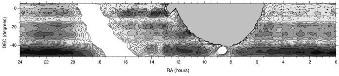
Figure 2: A sky map at 1465 MHz of a $60^{\circ}$ declination band obtained with the GEM experiment in the Southern Hemisphere using only a rim-halo protection and assuming an uniform baseline level across the sky (Epoch $2\,000.0$ coordinates). The pixelization is $1.6^{\circ}$ and the antenna temperature range extends 1.5 K above the lowest temperature in 12 equally-spaced contours in order to enhance the distribution of Galactic radiation away from the Galactic Plane.

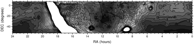
Figure 3: A GEM map at 1465 MHz of the same sky region as that in Fig. 2 (same baseline assumption and pixel size), but using data obtained after the wire mesh screen had been added to the shielding configuration of the antenna. The antenna temperature ranges also over 1.5 K above the lowest temperature, but the contour levels are spaced more tightly (60 mK). Marked locations denote the sky directions of the 6 test measurements discussed in Sect. 5.

Fig. 3 is a map of the same declination band as that of Fig. 2 after a fence of wire mesh had been built around the rotating antenna. A total of 222.57 hours of data from an optimally-stable receiver were used in the preparation of this map. The azimuth-dependent contamination from the ground has been largely removed and we can estimate its level by subtracting representative azimuth scans from the two maps as described below. No absolute calibration of the baseline was attempted for either of these maps, as it is not relevant for determining differential measurements. This approach will enable us to refine the model used in Sect. 5 for predicting a best estimate of the level of the azimuth-independent component of ground contamination in the survey. The locations marked in the map of Fig. 3 correspond to the chosen set of sky directions, grouped pair-wise, for obtaining the differential sky measurements. They avoid the proximity of the Galactic Plane in order to diminish the chance of scale error corrections.

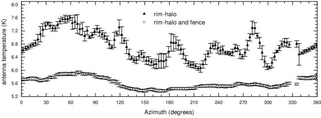
Figure 4: Antenna temperature profiles obtained before and after the construction of the fence and sampled along the scanning direction in regions of relatively low sky contrast.

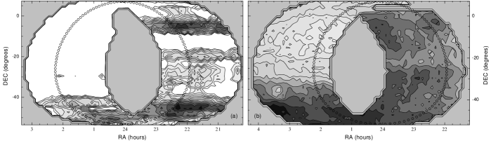
Figure 5: Maps of the sky regions revealed by the circularly scanning technique of the GEM experiment at 1465 MHz, (a) before and (b) after the construction of the fence, and the distribution of the alt-azimuth sky bins used in the sampling of the signal displayed in the antenna temperature profiles of Figs. 4a,b. Map (a) consumed 2.29 hours of observational time and Map (b) 2.18 hours. Both maps are given at a $1.6^{\circ}$ pixel-resolution and their antenna temperatures range in 12 contour steps of 60 mK above their respective minimum values.

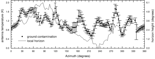
Figure 6: The level of ground contamination in the absence of the fence deduced from the difference in antenna temperature between the profiles of Fig. 4. The dotted line depicts the horizon profile at the observational site.

The variable or azimuth-dependent component of ground contamination can be estimated by adequate comparison of the azimuth antenna temperature profiles before and after the introduction of the fence. Fig. 4 shows two such sets of profiles. They were obtained from single time-ordered series of scans covering the same regions of the sky and they sample the sky in 122 alt-azimuthal circular bins spanning approximately half-a-beamwidth across. This binning criteria is a basic precept for the relative calibration of the survey and it will not be discussed further in the present context. A full treatment of this calibration technique can be found in Tello (Te1 (1997)) and will be included in the publication of the survey. At this point we just mention that the series of scans were chosen for complying with highly stable receiver performance and relatively high Galactic latitude. This combination favours sky profiles of low emission contrast for easier identification of the ground contribution to the antenna temperature. The circular arrangement of the sampled bins has been schematically superimposed against the observed sky in Figs. 5a,b. Thus the difference between the antenna temperature profiles in Fig. 4 is a good approximation (see Fig. 6) of the ground contamination in the absence of the fence. It can be seen to be made up of a variable component with a mean amplitude of $0.52\pm 0.29$ K above the level of a uniform azimuth-independent component. The two components result from the convolution of the antenna beam pattern over the ground temperature distribution, whose spatial extent in the vertical direction is limited by the line of the horizon also depicted in Fig. 6.

In the presence of the fence, we can estimate the azimuth-independent component of ground contamination by convolving the antenna beam pattern with an uniform field of radiation confined to the solid angle that the fence fills in at the prime focus of the parabolic dish. In this case, the beam pattern is the modified feed response which due to the presence of the shields gives rise to spillover and diffraction sidelobes. This is the subject we deal with in the next two sections before we assess the reality of the observations.

3 Feed pattern measurements

The antenna test range of the Integration and Tests Laboratory (a satellite dedicated facility) at the National Institute for Space Research – INPE – was used over a period of 3 weeks in order to obtain full beam patterns of the GEM backfire helical feed antennas at 408 MHz and 1465 MHz. For the measurements, a vertically polarized transmitter was located on a tower 25 m above the ground and 80 m in front of an anecoic chamber. The antenna under test sat on a plate attached to the head of the fiber glass support arm of a platform with 3 degrees of freedom (slide: horizontal motion along the axis between transmitting and receiving antennas; roll: rotation of the head support plate about the slide axis; azimuth: horizontal scanning motion).

During the measurements, the upper section of the support arm was surrounded with Eccosorb in order to avoid undesired strayed signal from the obstruction behind the head support plate. Furthermore, since a backfire helix radiates in the direction of its ground plane, PVC extensions were customized to position the helix upside down on the head plate and to direct the feed cable toward its connector at the ground plane. Preliminary tests were conducted at different positions along the slide axis to match the phase center of the feed antenna with the rotation axis of the support arm. The backlobe structures of the feeds were also obtained by adjusting their ground planes onto the PVC extensions attached to the head plate.

The beam patterns were obtained by measuring the power response of the antennas with polar angle $\theta$ while the platform rotated through $360^{\circ}$ in azimuth. The measurements were taken at $1.6^{\circ}$ intervals at 408 MHz and every $0.2^{\circ}$ at 1465 MHz. The full spatial response was generated by repeating the azimuth scans for a sequence of equally-spaced roll angles. Although a $180^{\circ}$ range in roll angle would have sufficed to cover all space directions, the helical antenna is capable of shifting the phase of the received signal as it turns around its main beam axis (Kraus Kra (1988)). Roll angle test measurements with the 408 MHz helix were consistent with this prediction and, in this case, the entire $360^{\circ}$ range in roll angle was covered at $4.8^{\circ}$ steps. No significant phase shifting was noticed with the 1465 MHz helix, for which $10^{\circ}$ roll angle steps were used.

As required by a polar angle resolution of $1^{\circ}$ in the diffraction model we apply in the next section, the measured responses were regridded and interpolated to accomodate a $1^{\tiny\squareforqed}$ spatial resolution. Diagrams of the resulting power patterns $P_{\rm n}(\theta,\phi)$ down to the 20-dB level are displayed in Figs. 7a,b. Their mean response averaged over $\phi$ produces the pattern profiles $P_{\rm n}(\theta)$ shown in Fig. 8. The radiometric characterization of these backfire helices is further illustrated in Fig. 9, showing the antenna solid angle as a function of the polar angle $\theta$, and Table 1 gives the directivity, $D$, main beam efficiency, $\epsilon_{\rm M}$, and the beam solid angle fraction, $\epsilon_{\rm h}$, intercepted by the co-rotating ground shield (halo) of the GEM parabolic reflector. The 10-dB points attain 93.8% and 62.5% of the total dish illumination at 408 MHz and 1465 MHz, respectively.

Figure 7: Diagram representations of the backfire power patterns at (a) 408 MHz and (b) 1465 MHz in a coordinate reference frame centered on the transmitter. Three concentric circles have been superimposed on the diagrams to illustrate the opening angles of the ground shields: the boundary of the dish itself at $\theta=78.9^{\circ}$, the rim-halo at $\theta=99.2^{\circ}$ and the farthest lying location on the upper edge of the fence at $\theta=142.9^{\circ}$ when $Z=45^{\circ}$. The 10-dB level is mostly contained inside the elliptical contour. Arrows indicate the $\phi^{\ast}(\equiv 180^{\circ}-\phi)$ orientations of the feed for generating the upper (upp) and lower (low) envelopes in Figs. 10–13. The subindex number denotes the number of shields accounted for (1 : only the rim-halo, 2 : both halo and fence).

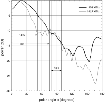
Figure 8: Polar diagrams of the 408 MHz and 1465 MHz feed patterns using the mean backfire response in the $\phi$-plane. Vertical reference lines delimit the sidelobe structure within the field of view of the halo and the width of the assumed main beams.

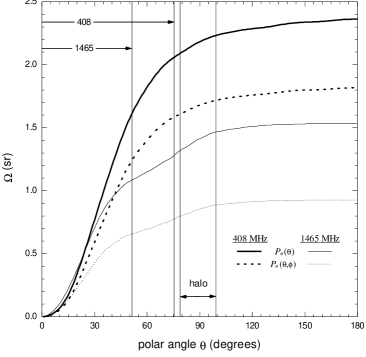
Figure 9: Antenna solid angle growth with polar angle for the beam patterns in Fig. 8 and for the full 3-d measured response of the backfire feeds. The vertical lines are as in Fig. 8.

Table 1: Measured radiometric properties of backfire helical feeds

	$P_{\rm n}(\theta)$			$P_{\rm n}(\theta,\phi)$
	408 MHz	1465 MHz		408 MHz	1465 MHz
$D$	5.32	8.19		6.92	13.56
$\epsilon_{\rm M}$	0.87	0.71		0.87	0.71
$\epsilon_{\rm h}\times 10^{2}$	5.90	9.36		5.89	9.32

Experimental reports on monofilar axial-mode helical antennas have seldom focused the backfire type. End-fire helices of equivalent design characteristics, for example, do not depend critically on frequency over the range studied here (see Paper I); whereas Table 1 clearly favours a frequency dependence for the backfire mode. A few authors have also attempted to describe the radiometric properties of the backfire helix from analytical, numerical and experimental points of view (Sexson Sex (1965); Johnson & Cotton JC (1984); Nakano et al. NYM (1988)). No definite consensus has yet emerged from these studies, since the mechanical design of the helices under investigation was substantially different for each author. Our backfire feeds, which follow the design considerations of typical Kraus coils (Kraus Kra (1988)), show a substantial narrowing of the beamwidth with increasing frequency which disagrees with the predictions of earlier studies (Sexson Sex (1965); Nakano et al. NYM (1988)).

4 Analysis of ground contamination

In the long-wavelength regime of the GEM experiment, there are two main sources of contamination, aside from Galactic stray radiation, which affect invariably the antenna noise temperature of the sky. These are the emissions of the ground and the atmosphere. The latter, being a factor of at least 20 dB smaller than the former, can be safely considered to be an elevation-dependent contribution to the signal level of the main beam. The ground contamination, on the other hand, requires a precise knowledge of the spillover and diffraction sidelobes of the feed in order to discriminate its contribution to the overall antenna noise temperature. In this section, we apply the geometric diffraction model developed in Paper I in order to account for the effect of shielding in the estimates of the ground signal. The shields are (see Fig. 1) a 5-m high fence, inclined at $50^{\circ}$ from the ground and standing at 6.4 m from the pivot point of the dish, and a halo of aluminum panels extending 2.1 m from the dish petals. The fence attenuation was estimated at the 10-dB level for 408 MHz radiation, but below 1 dB at 1465 MHz.

4.1 Model predictions

Our analytical tools enable us to estimate, as a function of the zenith angle $Z$, the amount of ground contamination due to the unshielded and diffracted components. The estimates, in units of antenna temperature, are given according to Fresnel and Fraunhofer diffraction theories in order to test for near and far-field effects in the range $0^{\circ}\leq Z\leq 45^{\circ}$. The asymmetry of the feed patterns introduces an additional complication, since the solid angle over which the ground temperature is distributed (assumed to be the field of view below the upper edge of the fence) is seen through a sidelobe structure that depends on the orientation of the $\phi$-plane of the feed. Therefore, a family of 24 profiles was prepared for each feed by rotating the $\phi$-plane in $15^{\circ}$ steps around the beam axis. For a tilted dish, the $\phi=0^{\circ}$ reference directions of Fig. 7 correspond to the line of sight which clears off the edge of the halo at the smallest $Z$ angle. Figs. 10 and 11 display the model estimates assuming a 10 dB attenuation from the fence (as in the 408 MHz case) in the presence and absence of the halo, respectively. Figs. 12 and 13 describe the situation of the 1465 MHz channel, for which the model fence provides no significant attenuation. The upper and lower envelopes of each family of profiles have been identified along with some other profiles. The orientations of the 408 MHz and 1465 MHz feed patterns that produce these upper and lower envelopes are indicated with labelled arrows in Fig. 7.

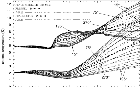
Figure 10: Predicted antenna noise temperature due to transmitted and diffracted ground radiation in a one-shielded (fence) GEM experiment at 408 MHz. The diffracted components were calculated in both the Fresnel (thin lines) and the Fraunhofer (thick lines) regimes. The beam pattern asymmetry of the backfire helices gives rise to families of profiles, some of which have been labelled according to the $\phi$-plane orientation of the feed. All the profiles fall into 4 sets, each of which has been drawn according to the sequence of line types indicated by $P_{\rm n}(\theta,\phi)$.

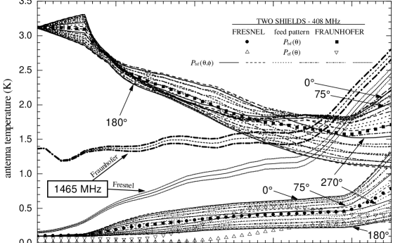
Figure 11: Predicted antenna noise temperature due to transmitted and diffracted ground radiation in the double-shielded GEM experiment at 408 MHz. Two additional triple-sets of profiles have been included to show the Fresnel and Fraunhofer estimates at 1465 MHz for $\phi=12^{\circ}$ using a $7.91(^{+0.35}_{-0.32})$-dB attenuating fence and raised 80 cm above the ground as discussed in Sect. 5.2. Legend and label explanations are as in Fig. 10.

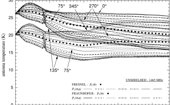
Figure 12: Predicted antenna noise temperature due to transmitted and diffracted ground radiation in a one-shielded (no halo) GEM experiment at 1465 MHz. Legend and label explanations are as in Fig. 10. Since the assumed attenuation of the fence is small, $0.3$ dB, the plotted profiles represent an effectively unshielded case.

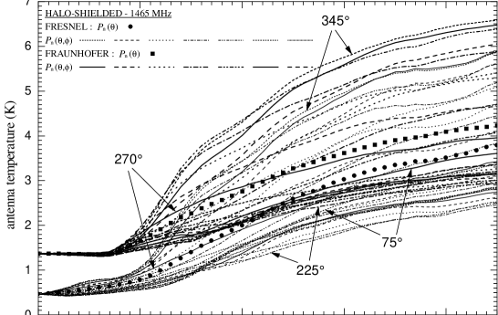
Figure 13: Predicted antenna noise temperature due to transmitted and diffracted ground radiation in the double-shielded GEM experiment (an effectively one-shielded, fenceless, configuration) at 1465 MHz. Legend and label explanations are as in Fig. 10.

4.2 Ground contamination scenarios

Figs. 10 through 13 characterize four types of ground contamination scenarios: (1) fence-shielded in Fig. 10, (2) double-shielded in Fig. 11, (3) unshielded in Fig. 12 and (4) halo-shielded in Fig. 13. The distinction is clear enough to show how the amount of shielding and the wavelength-dependent strength of the diffraction effects shape the ground contamination profiles. Thus, as we proceed from a weakly-diffracting and unshielded antenna scenario to a strongly-diffracting and double-shielded one, far-field diffraction effects give way to near-field ones. In doing so, the distance-dependent calculations with the Fresnel approach become more difficult to be matched by the Fraunhofer approximations, whose typical overestimating power is further increased.

Shielded scenarios produce also profiles with a tendency to resemble the underlying variation of the solid angle that exposes the ground for a given $Z$ (see Fig. 6 in Paper I). In particular, when $Z$ is large enough to expose unscreened ground below the fence, the corresponding profile shows a marked increase in ground signal. It should be noted that the profiles obtained with the Fraunhofer formalism in the double-shielded scenario of Fig. 10 deviate from these generalized description, since one expects the role of near-field diffraction at the longer wavelength and at the innermost shield to become significant.

The composition of the ground contamination profiles in terms of their transmitted and diffracted components can also be investigated by analyzing the symmetrized responses $P_{\rm n}(\theta)$. The diffraction model that we are using does not produce, however, separate estimates of transmitted and diffracted components in the Fresnel regime. Unlike in the Fraunhofer regime, where both components are obtained independently, the Fresnel convolution integral for calculating the contamination by the halo (or of the dish in the unshielded scenario) produces a transmission-embedded result. Nevertheless, in order to obtain an equivalent form of diffraction component, we have subtracted from the convolved result the same transmitted component as in the Fraunhofer regime. In a very realistic sense, the definition of a spillover sidelobe reduces to the sidelobe level that is not modified by the presence of a physical obstruction along the line of sight of the feed and within the angular range of the ground temperature distribution. This analytical construct allows us to plot in Fig. 14 the ratio $R_{t}$ of the transmitted component to the total ground contamination in the Fresnel regime.

The reason why the unshielded scenario in Fig. 14 produces anomalous $R_{t}>1$ values is a consequence of the above given definition for the spillover component. This definition implies that the diffraction sidelobes (whose sidelobe level is modified) can actually suppress, rather than enhance, the spillover ones. From the point of view of a Fresnel diffraction pattern, this behavior is readily understood as the restriction imposed by the ground temperature distribution on the angular range spanning the relative power response of the feed. The restriction sets effectively an upper cut-off in the amplitudes of the crests that characterize the rippling profile of this response (see, for example, Fig. 4 in Paper I). Thus, if the cut-off is sufficiently low the overall relative power response can fall below unity. This spillover suppression is also present in the other scenarios, but is not dominant and, as expected from the geometrical argument above, it originates in the portion of the halo or dish hidden from the outside by the structure of the fence. The effect is stronger in the absence of the shields and it becomes more pronounced at the shorter wavelength. Similar calculations with a relatively lower sidelobe structure also demonstrated that in order for spillover suppression to set in, the level of the relevant sidelobes cannot be made arbitrarily small.

Although transmission dominates the ground contamination at large $Z$, the $R_{t}$ curves in Fig. 14 indicate that diffraction becomes the dominant component at lower $Z$ as the amount of shielding is also increased. We can quantify the relevance of the spillover sidelobes by introducing a transmission factor $Q_{\rm n}$ (the normalized integral under the $R_{t}$ curves). Accordingly, a thoroughly spillover-dominated scenario would result in $Q_{\rm n}=1$, whereas a fully diffraction-dominated case would yield $Q_{\rm n}=0$. Table 2 lists the transmission factor in the four shielding scenarios analyzed in this section. Only the double-shielded scenario may be recognized to be dominated by the diffraction sidelobes.

Finally, it should be stressed that the estimates given in this section have assumed from the start that the ground temperature distribution is an isotropic field of radiation regardless of the horizon profile. As we saw in Sect. 2 this assumption is a valid one for a contaminating signal free of horizon-dependent variations, i.e. for a truly effective double-shielded scenario. Although possible, but not desirable for experimental reasons (horizontally striped maps), the convolution of the beam pattern with an anisotropic ground temperature distribution would yield a more realistic estimate in the other three scenarios. In these cases, a set of profiles like the ones shown in Figs. 10, 12 and 13 would have to be assembled for each particular azimuth.

Table 2: Transmission factor $Q_{\rm n}$

feed		Effective Shielding
regime		none	fence	halo	double
Fresnel		0.98	0.80	0.70	0.41
Fraunhofer		0.82	0.34	0.55	0.10

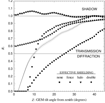
Figure 14: The four ground contamination scenarios in terms of the ratio $R_{t}$ of the transmitted component to the total ground contamination in the Fresnel regime. In the shadow region, spillover suppression by the diffraction sidelobes nearest to the ground dominate the diffracted component. The line and dotted curves mark the double-shielded case at 1465 MHz discussed in Sect. 5.3.

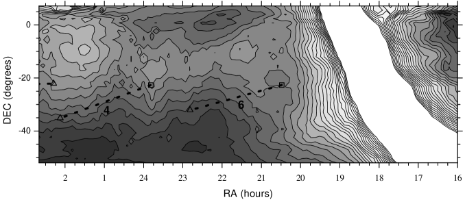
Figure 15: Destriped partial map at $1.6^{\circ}$-pixel resolution of the high-sampled sky regions displayed in the declination band of Fig. 3. The antenna temperature range is 1.5 K in 60 mK contour steps. Squared and triangular symbols denote, respectively, the sky directions of the paired $Z=90^{\circ}$ and $Z=60^{\circ}$ observations for the test measurements.

5 Test measurements

A series of dedicated measurements was conducted with the GEM radiotelescope at 1465 MHz during the present observational period in Brazil in order to improve the discrimination of the sky contaminating sources. The measurements consisted of pairs of observations taken at $Z=0^{\circ}$ and at $Z=30^{\circ}$ in sky directions away from the Galactic Plane (see Fig. 3). Each observation sampled the radiometric signal every 0.56 seconds over a few minutes while an approximate 15-minute interval elapsed between the $Z=0^{\circ}$ and the $Z=30^{\circ}$ samplings. In this manner, a total of 6 measurements were obtained over a nearly 3-month period. Although the absolute level of ground contamination in general will be somewhat different for different pairs, the mean difference between the two levels, $\bar{\Delta}T_{\rm A}$, can be used for comparison with the model predictions outlined in the preceding section.

This differential measurement approach relies, however, on our ability to separate likewise the other constituents of the antenna noise temperature, namely, the atmospheric emission and the sky background. The latter is a mixture of synchrotron and free-free radiation originating in the Galaxy, Cosmic Microwave Background Radiation (CMBR) and a diffuse background of extragalactic origin. Depending on the sky direction Galactic emission at 1465 MHz can be some 5 times larger or even a full order of magnitude smaller than the signal due to the CMBR. The atmospheric contribution, on the other hand, is necessarily larger at $Z=30^{\circ}$ than at the zenith because of a larger air mass. At 1465 MHz the bulk of the emission by the atmosphere is due to the pressure-broadened spectra of the O₂ molecule. Using the reference model proposed by Danese and Partridge (DP (1989)) (see also Liebe Lie (1985) and Staggs et al. Sta (1996)) a straightforward secant law correction to the zenith contribution at the Brazilian site gives an estimate for the differential atmospheric component of $0.305\pm 0.090$ K.

5.1 Data reduction

Our data was first time-ordered and corrected for thermal susceptabilities of the receiver baseline ($0.3591\pm 0.0007$ K/^∘C) and fractional gain ($0.00922\pm 0.00001/^{\circ}$C). Then, 44.8-second bursts of 2.24-second firings of a thermally stable noise source diode were extracted from the data stream and used to calibrate the overall system gain. Table 3 summarizes the results of the observations along with the number of samples and the implied differences in antenna temperature between the two $Z$ directions for: (i) the measurements, (ii) the Galactic emission background and (iii) the final budget (including the increase due to the larger optical depth of the atmosphere at $Z=30^{\circ}$). The Galactic contribution was estimated using a partial map (65.21 hours of data) of the sky signal from the GEM experiment at 1465 MHz, whose baseline has been so far properly corrected according to a destriping algorithm in order to filter out low frequency noise (Tello Te1 (1997)). The data for this map makes up about 30% of the data used in preparing the map in Fig. 3, but due to sampling differences (which bias the destriping process – see also Table 4) it has been split into the two maps shown in Figs. 15 and 16 along with the locations chosen for the paired measurements listed in Table 3.

Table 3: Antenna temperature in the GEM experiment at 1465 MHz for observations at $Z=0^{\circ}$ and $30^{\circ}$.

		$Z=0^{\circ}$			$Z=30^{\circ}$			$\Delta T_{\rm A}$ (K)
pair		$T_{\rm A}\pm 1\sigma$ (K)	$N$		$T_{\rm A}\pm 1\sigma$ (K)	$N$		measurement	Galaxy	final budget
1		$10.798\pm 0.042$	104		$12.151\pm 0.035$	150		$1.353\pm 0.055$	$-0.083\pm 0.035$	$0.97\pm 0.11$
2		$9.620\pm 0.036$	146		$11.028\pm 0.036$	93		$1.408\pm 0.051$	$-0.254\pm 0.066$	$0.85\pm 0.12$
3		$11.212\pm 0.040$	219		$12.180\pm 0.046$	347		$0.967\pm 0.061$	$+0.307\pm 0.043$	$0.97\pm 0.12$
4		$7.923\pm 0.035$	71		$9.299\pm 0.040$	148		$1.376\pm 0.054$	$+0.173\pm 0.050$	$1.24\pm 0.12$
5		$8.922\pm 0.030$	132		$10.151\pm 0.031$	82		$1.229\pm 0.043$	$-0.028\pm 0.011$	$0.90\pm 0.10$
6		$12.472\pm 0.038$	131		$13.582\pm 0.039$	267		$1.110\pm 0.054$	$+0.185\pm 0.024$	$0.99\pm 0.11$

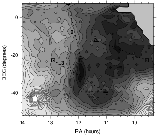
Figure 16: The low-sampled complement of the map in Fig. 15, but at the same resolution and with the same gray scaling in antenna temperature. The upper-right hand corner is data defficient due to $60^{\circ}$ custom cuts around the Sun.

In order to extract the antenna temperature in a given direction, the pixel nearest to it was found first and then averaged with the surrounding set of 8 neighbouring pixels taken at half-weights. This procedure allows us to sample the sky in a square region $4.8^{\circ}$ ($1.6^{\circ}$ per pixel) on the side and is consistent with a HPBW of $\approx 5.4^{\circ}$ for the 1465 MHz beam (Tello Te1 (1997)). This can also be verified in Table 4 where we compare these estimates with those of the nearest pixel value itself and the average from the 4-pixel area enclosing the given direction along with the sampling differences among the different pairs. Note that pair 5 is actually missing in Fig. 15 and, therefore, we have provisionally supplemented the data in Tables 3 and 4 with the differential measurement obtained using the map in Fig. 3. To see that this is not as bad as it appears, the mean absolute difference between the estimates for pairs 1, 2 and 3 in the maps of Figs. 3 and 16 (low-sampled sky) is $0.237\pm 0.066$ K, but only $0.112\pm 0.040$ K for pairs 4 and 6 in the high-sampled regions of the map in Fig. 15. Thus, within the sensitivity of our measurements ($\approx 20$ mK) the Galactic contributions to the differential measurements in Table 3 turn out to be smaller than, or as large as, the one estimated for the emission of the atmosphere.

Table 4: Effects of binning strategy for the Galactic contribution to differential measurements at 1465 MHz^a

		1-pixel				4-pixel matrix				9-pixel matrix
pair		$\Delta T_{\rm A}$ (K)	$N_{90}$	$N_{60}$		$\Delta T_{\rm A}\pm 1\sigma$ (K)	$N_{90}$	$N_{60}$		$\Delta T_{\rm A}\pm 1\sigma$ (K)	$N_{90}$	$N_{60}$
1		$-0.100$	13	9		$-0.078\pm 0.032$	48	39		$-0.083\pm 0.035$	110	92
2		$-0.288$	4	63		$-0.257\pm 0.026$	14	233		$-0.254\pm 0.066$	33	338
3		$+0.254$	18	11		$+0.325\pm 0.034$	74	56		$+0.307\pm 0.043$	165	120
4		$+0.222$	70	47		$+0.217\pm 0.023$	293	203		$+0.173\pm 0.050$	697	428
5		$-0.008$	160	252		$-0.019\pm 0.006$	637	997		$-0.028\pm 0.011$	1419	2179
6		$+0.178$	63	85		$+0.177\pm 0.023$	251	343		$+0.185\pm 0.024$	568	784
$\bar{\Delta}T_{\rm A,\oplus}^{\rm obs}$		$1.003\pm 0.071^{\mathrm{b}}$				$0.983\pm 0.046\pm 0.054$				$0.992\pm 0.044\pm 0.062$

• The entries referred to as $N_{90}$ and $N_{60}$ correspond to the number of observations sampled in the

• determination of the sky signal observed toward $Z=90^{\circ}$ and $Z=60^{\circ}$, respectively.

• Only the external error ($\sigma/\sqrt{5}$) has been assigned in this case.

The weighted average of the values in the last column of Table 3 is an estimate of the differential ground contamination in the GEM experiment at 1465 MHz. We obtain $\bar{\Delta}T_{\rm A,\oplus}^{\rm obs}=0.992$ K with internal and external 1-$\sigma$ error estimates of 0.044 and 0.062 K, respectively (see also Table 4). Based on the ratio between these two errors, we can rule out the presence of systematic errors, which may have been introduced, for instance, by unaccounted stray radiation contamination of sidelobes other than those considered here. In fact, aside from the differential measurement approach, which reduces the effect of of residual sidelobe contamination, the signal contrast of even the brightest sky features relative to that of the ground does not go above the 13-dB level. Only the presence of the Sun could offer potential problems, but except for pair 1, none of the other measurements was conducted with the Sun above the horizon. Still, the estimate from pair 1 does not raise suspicious concerns, eventhough the Sun was seen at $90.0^{\circ}$ from axis and at $71.2^{\circ}$ during the observations toward $Z=60^{\circ}$ and $Z=90^{\circ}$, respectively.

5.2 Orientation of the $\phi$-plane

Before attempting a comparison of $\bar{\Delta}T_{\rm A,\oplus}^{\rm obs}$ with our model predictions, we need to assign the orientation of the $\phi$-plane of the feed in order to select the most likely profile. In addition, we have to apply the model calculations for the shield configuration actually used during the observations. Although the halo was the same as the one assumed to obtain the results in Figs. 10 through 13, the attenuation of the fence was increased by using a wire mesh with holes half as small and wires 25% thinner (according to our attenuation formula in Paper I we should thereby obtain a 6.2-dB screening effect at 1465 MHz). Finally, the entire fence was raised 80 cm above the ground.

The orientation of the $\phi$-plane of the feed could be inferred by direct comparison of the feed diagram in Fig. 7b with the mapping of the beam pattern of the antenna by some convenient point source. This procedure is, of course, based on the assumption that the feed axis is also not perfectly aligned with the optical axis of the secondary for an asymmetric beam pattern to be projected onto the sky. In our case we chose the Sun, at a particular time of the year, which at the Brazilian site can be made to intercept the Galactic scans at $Z=30^{\circ}$ with sufficient angular coverage ($\sim 30^{\circ}$) around the beam axis. The result of such a mapping is displayed in Fig. 17 in 20 contour steps of 1 dB. The brightest region, corresponding to the precise passage of the scan circle through the Sun, could not be mapped up to a true 0-dB level because the signal overshot the detector threshold. This may have caused the double-lobed structure seen inside the main beam pattern in Fig. 7b to smooth out in the mapping of Fig. 17. In fact, in 1994, when the solar activity was relatively low, we recorded a solar transit (see Fig. 18) in Bishop, CA, which did not saturate the detector and did reveal a double-peaked main beam. In Fig. 17 the innermost contours follow the outlines of a bulged shape which is reminiscent of the double-lobed structure. Thus, together with the ellipticity of the surrounding contours in both diagrams we determined the $\phi$-plane orientation of the feed from the difference in the orientation of the major axis of these elliptical contours. The 10-dB contours are well confined inside elliptical boundaries with eccentricities of 0.64 and 0.34 for the feed and antenna patterns, respectively. The semi-major axis of the ellipse in the direction of the larger lobe in Fig. 7b is then oriented along $\phi=125^{\circ}$ while that in the direction of the bulged region in Fig. 17 corresponds to $\phi^{\ast}=317^{\circ}$. Since $\phi^{\ast}\equiv\phi+180^{\circ}$, according to the system of coordinates used in Fig. 17, we obtain a $\phi$-plane orientation for the feed of $12^{\circ}$.

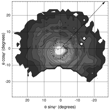
Figure 17: Beam pattern mapping of the 1465 MHz backfire-fed GEM antenna, in twenty 1-dB steps and at a pixel resolution of at $1.6^{\circ}$, using the passage of the Sun through the $Z=30^{\circ}$ scan circles of the antenna on the 29-th of September 1999 in Cachoeira Paulista, Brazil. The $\phi^{\ast}$ angle of the pattern is measured counterclockwise from the ordinate axis and corresponds to $\phi-180^{\circ}$ in the coordinate system of Fig. 7b while the elevation of the Sun is given by $60^{\circ}-\theta\cos\phi^{\ast}$. The arrow indicates the major axis alignment of the 10-dB elliptical contour toward the larger component of the double-lobed structure in Fig. 7b.

Figure 18: Antenna noise temperature record (solid line) of a solar transit in Bishop, CA, during data taking operations at 1465 MHz in October 1994. The elevation of the Sun, $H_{\rm Sun}$, is given by the dotted line. The peaks A and B indicate relative maxima in the antenna response and span an $\approx 5^{\circ}$ interval in the azimuth coordinate of the Sun.

5.3 Final estimates

Our diffraction model predicts a differential ground contamination of $\Delta T_{\rm A,\oplus}=1.380$ K for the shield configuration used during the observations and an orientation of $\phi_{\rm plane}=12^{\circ}$. In order to predict the observed value of $\bar{\Delta}T_{\rm A,\oplus}^{\rm obs}$, we have to adjust the attenuation coefficient of the wire mesh by an efficiency factor $\beta=0.675\pm 0.052$ or, equivalently, increase the screening of the fence by $1.71^{+0.35}_{-0.32}$ dB. The resultant profile has been included in Fig. 11. $\beta$ scales linearly not only with $\Delta T_{\rm A,\oplus}$, but also with the predicted differential ground contributions from the halo, $\Delta T_{\rm A,\oplus}^{\rm\,hal}$, and from the fence, $\Delta T_{\rm A,\oplus}^{\rm\,fen}$. So, if

$${\beta\over 10^{-3}}=-155.880+837.363\,\left({\Delta T_{\rm A,\oplus}\over{\rm K}}\right)\;,$$ (1)

then the corresponding contributions from the halo and from the fence are

$$\left({\Delta T_{\rm A,\oplus}^{\rm\,hal}\over{\rm mK}}\right)=31.49-169.25\,\left({\Delta T_{\rm A,\oplus}\over{\rm K}}\right)$$ (2)

and

$$\left({\Delta T_{\rm A,\oplus}^{\rm\,fen}\over{\rm mK}}\right)=193.61-40.00\,\left({\Delta T_{\rm A,\oplus}\over{\rm K}}\right)$$ (3)

with 1-$\sigma$ errors of 0.03 and 0.01 in the zero-points and linear coefficient, respectively, in (2) and (3); but 1 order of magnitude smaller in those of (1).

These formulae tell us that, as the screening of the fence becomes less efficient ($\beta$ increasing), the differential ground contribution increases, eventhough the one from the diffracted components decreases. In this spillover-dominated scenario with $Q_{\rm n}=0.67\pm 0.01$ (see Fig. 14) the ground contamination contributed by diffraction at the halo and at the fence will decrease with increasing $Z$ as long as $\beta\,\raise 1.07639pt\hbox{$>$}\hskip-6.99997pt\raise-1.93747pt\hbox{$\scriptstyle\sim$}\hskip 1.99997pt\,0.00011$ and $\beta\,\raise 1.07639pt\hbox{$>$}\hskip-6.99997pt\raise-1.93747pt\hbox{$\scriptstyle\sim$}\hskip 1.99997pt\,3.9$, respectively. For most practical fences, the lower bound on $\beta$ implies that diffraction at the halo should always decrease with $Z$. In order to have the same scenario at the fence, the attenuation of the wire mesh would have to be quite low ($\,\raise 1.07639pt\hbox{$<$}\hskip-6.99997pt\raise-1.93747pt\hbox{$\scriptstyle\sim$}\hskip 1.99997pt\,0.3$ dB).

Table 5 gives the refined model estimates of the ground contamination levels for GEM observations at 1465 MHz in the Southern Hemisphere.

Table 5: Ground contamination in $Z=30^{\circ}$ GEM data at 1465 MHz from the Southern Hemisphere.

sidelobe	shielda		contamination		error
			(mK)		(mK)
spillover	double		975		75
diffraction	fence		154		3
diffraction	halo I		28		2
diffraction	halo II		-11		1
Total	double		1146		75

• Estimates are given for a double-shielded scenario were the rim-halo contribution to the diffracted component has been separated into exposed (halo I) and hidden (halo II) portions as discussed in Sect. 4.2.

6 Summary and conclusions

Levelling and reducing the contamination of the antenna temperature by ground emission is an important requirement in survey experiments for mapping the non-thermal component of the Galactic emission background. In the zenith-centered 1-rpm circular scans of the GEM experiment this is achieved by using a wire mesh fence around a rim-halo shielded antenna. Without the fence, a prohibitive variable component of ground contamination compromises the data taken with this portable 5.5-m dish in the Southern Hemisphere at 1465 MHz with a mean amplitude of $0.52\pm 0.29$ K above the level of a uniform azimuth-independent component. With the fence, the level of a uniform component was obtained by comparing differential measurements of the antenna temperature toward selected regions of the sky with model predictions of the spillover and diffraction sidelobes.

First of all, the model allowed us to investigate the shielding performance of the experiment using the fully measured beam patterns of the GEM backfire helical feeds at 408 MHz and 1465 MHz. We concluded that far-field diffraction effects dominate a weakly-diffracting and unshielded antenna scenario whereas near-field effects dominate a stronger-diffracting and double-shielded scenario. Furthermore, the shielding efficiency of the experiment could be quantified in terms of the normalized cumulative ratio $Q_{n}$ of the spillover-induced transmission to the overall sidelobe contamination in the zenith angle range $0^{\circ}\leq Z\leq 45^{\circ}$. If the shielding is low enough, spillover sidelobe suppression will ensue, since the ground temperature angular distribution can introduce an upper cut-off in the relative power response of the feed. A critical element in the analysis is introduced, however, by the need to account for the assymetric response of the feed and which seems, most likely, to result from imperfect alignment of the feed axis on the measuring stand and along the optical axis of the secondary. We used the near sidelobe pattern (out to some $30^{\circ}$ from axis) of the radiotelescope to ressolve the issue.

Finally, we applied atmospheric and Galactic corrections to the differential measurements before comparing the residual signal with the model predictions for the level of ground contamination. The choice of sky directions away from the Galactic Plane led to contributions from the sky between $Z=0^{\circ}$ and $Z=30^{\circ}$ which were as high, but not larger, than the ones expected from the emission of the atmosphere. The former were derived from a template sky with a sensitivity of 20 mK based on GEM data taken at 1465 MHz in the Southern sky with a HPBW$\approx 5.4^{\circ}$.

The corrected test measurements match the model predictions if we introduce a screening efficiency factor $\beta$ which shows strict and separate linear correlations with the differential ground contamination and its diffraction components generated at the shields. Consequently, it suffices that the (total) differential ground contamination be known, for its spillover and diffracted components to be identified uniquely. With the refined model ($\beta=0.675\pm 0.052$) a uniform level of ground contamination is estimated at $1.146\pm 0.075$ K with a spillover-to-diffraction component ratio of $5.7\pm 0.5$. This is a spillover dominated scenario with $Q_{\rm n}=0.67\pm 0.01$ and decreasing diffraction sidelobes with increasing $Z$.

- (1) Banday A.J., Wolfendale A.W., 1991, MNRAS 248, 705
- (2) Bennett C.L., Smoot G.F., Hinshaw G., et al., 1992, ApJ 396, L7
- (3) Bennett C.L., Smoot G.F., Hinshaw G., et al., 1996, ApJ 464, L1
- (4) Berkhuijsen E.M., 1972 , A&AS 5, 263
- (5) Danese L., Partridge R.B., 1989, ApJ 342, 604
- (6) Davies R.D., Gutierrez C.M., Hopkins J., et al., 1996a, MNRAS 278, 883
- (7) Davies R.D., Watson R.A., Gutiérrez C.M., 1996b, MNRAS 278, 925
- (8) De Amici G., Torres S., Bensadoun M., et al., 1994, ApSS 214, 151
- (9) Delabrouille J., 1998, A&AS 127, 555
- (10) Gundersen J.O., Lim M., Staren J., et al., 1995, ApJ 443, L57
- (11) Hartmann D., Kalberla P.M.W., Burton W.B., Mebold U., 1996 A&AS 119, 115
- (12) Hartmann D., Burton W.B., 1997 Atlas of Galactic Neutral Hydrogen. Cambridge University Press.
- (13) Haslam C.G.T., Quigley M.J.S., Salter C.J., 1970, MNRAS 147, 405
- (14) Haslam C.G.T., Wilson W.E., Graham D.A., Hunt G.C., 1974, A&AS 13, 359
- (15) Haslam C.G.T., Klein U., Salter C.J., et al., 1981, A&AS 100, 209
- (16) Johnson R.C., Cotton R.B., 1984, IEEE Trans. Antennas Propagat. 32, 1126
- (17) Jones A.W.: 1999, Foregrounds and experiments below 33 GHz. In: de Oliveira-Costa A., Tegmark M. (eds.) Microwave Foregrounds. PASPC 181, 321
- (18) Kogut A., Banday A.J., Bennett C.L., et al., 1996a, ApJ 460, 1
- (19) Kogut A., Banday A.J., Bennett C.L., et al., 1996b, ApJ 464, L5
- (20) Kraus J.D., 1988, Antennas, McGraw-Hill, New York, Chap. 7
- (21) Lawson K. D., Mayer C. J., Osborne J. L., Parkinson M.L., 19987, MNRAS 225, 307
- (22) Liebe H.J., 1985, Rad. Sci. 20(5), 1069
- (23) Lim M., Clapp A.C., Devlin M.J., et al., 1996, ApJ 469, L69
- (24) López-Corredoira M., 1999, A&A 346, 369
- (25) Maino D., Burigana C., Gorski K., et al., 1999, A&AS 140, 383
- (26) Nakano H., Yamauchi J., Mimaki H., 1988, IEEE Trans. Antennas Propagat. 36(10), 1359
- (27) Platania P., Bensadoun M., Bersanelli M., et al., 1998, ApJ 505, 473
- (28) Reich W., 1982, A&AS 48, 219
- (29) Reich P., Reich W., 1986, A&AS 63, 205
- (30) Sexon T.L., 1965, Sylvannia Electron. Syst. Rep. ASTIA Doc. 626088
- (31) Smoot G.F., Bennett C.L., Kogut A., et al., 1992, ApJ 396, L1
- (32) Smoot G.F.: 1999, CMB synchrotron foreground. In: de Oliveira-Costa A., Tegmark M. (eds.) Microwave Foregrounds. PASPC 181, 61
- (33) Staggs S.T., Jarosik N.C., Wilkinson D.T., Wollack E.J., 1996, ApJ 246, 407
- (34) Tello C., 1997, Um experimento para medir o brilho total do céu em comprimentos de onda centimétricos, Tese de doutorado, Instituto Nacional de Pesquisas Espaciais, São José dos Campos, SP, Brasil
- (35) Tello C., Villela T., Wuensche C.A., et al., 1999, Rad. Sci. 34(3), 575
- (36) Torres S., Cañon V., Casas R., et al., 1996, ApSS 240, 225