Orbital Structure of Triaxial Black-Hole Nuclei

Abstract

Orbital motion in triaxial nuclei with central point masses, representing supermassive black holes, is investigated. The stellar density is assumed to follow a power law, $\rho\propto r^{-\gamma}$, with $\gamma=1$ or $\gamma=2$. At low energies the motion is essentially regular; the major families of orbits are the tubes and the pyramids. Pyramid orbits are similar to box orbits but have their major elongation parallel to the short axis of the figure. A number of regular orbit families associated with resonances also exist, most prominently the banana orbits, which are also elongated parallel to the short axis. At a radius where the enclosed stellar mass is a few times the black hole mass, the pyramid orbits become stochastic. The energy of transition to this “zone of chaos” is computed as a function of $\gamma$ and of the shape of the stellar figure; it occurs at lower energies in more elongated potentials. Our results suggest that supermassive black holes may place tight constraints on departures from axisymmetry in galactic nuclei, both by limiting the allowed shapes of regular orbits and by inducing chaos.

Astrophysical Journal, Vol. 549, Number 1, Part 1, Page 192

1 Introduction

An important change in our thinking about galaxy dynamics took place during the last decade, when it was recognized that the central densities of early-type galaxies and spheroids are generically very high. Evidence for large central masses came from high-resolution kinematical studies of nuclear stars and gas, which revealed the presence in roughly a dozen galaxies of compact dark objects with masses $10^{6.5-9.5}M_{\odot}$, presumably supermassive black holes (Ford et al. (1998)). Observations with HST also demonstrated very high stellar densities at the centers of early-type galaxies (Crane et al. (1993); Ferrarese et al. (1994)). Low luminosity ellipticals have density profiles that increase as unbroken power laws at small radii, $\rho\sim r^{-\gamma}$, with $\gamma\approx 2$. But Kormendy pointed out already in 1985 that bright galaxies also have central brightness profiles that deviate systematically from that of an isothermal core. The significance of this deviation was not recognized for ten more years due to an optical illusion associated with projection onto the plane of the sky. A luminosity density that varies as $r^{-\gamma}$ at small radii generates a power-law cusp in projection only if $\gamma>1$. When $\gamma=1$, the central surface brightness is logarithmically divergent (e.g. Dehnen (1993), Fig. 1), and the surface brightness profile differs only subtly from that of a galaxy with an isothermal core. Nonparametric deprojection of the luminosity profiles of bright galaxies (Merritt & Fridman (1995); Gebhardt et al. (1996)) revealed that they too harbor power-law cusps but with indices $\gamma\mathrel{\mathchoice{\lower 3.6pt\vbox{\halign{$\mathsurround=0pt\displaystyle\hfil#\hfil$\cr<\crcr\sim\crcr}}}{\lower 3.6pt\vbox{\halign{$\mathsurround=0pt\textstyle\hfil#\hfil$\cr<\crcr\sim\crcr}}}{\lower 3.6pt\vbox{\halign{$\mathsurround=0pt\scriptstyle\hfil#\hfil$\cr<\crcr\sim\crcr}}}{\lower 3.6pt\vbox{\halign{$\mathsurround=0pt\scriptscriptstyle\hfil#\hfil$\cr<\crcr\sim\crcr}}}}1$.

While the origin of the power-law cusps is not clear, there are hints that they may be associated with black holes. Steep cusps, $\gamma\approx 2$, form naturally in stellar systems where the black holes grow on time scales long compared to crossing times (Peebles (1972); Quinlan, Hernquist & Sigurdsson (1995)). No universally accepted model has yet been proposed for the origin of the weak cusps, but we note here one feature that suggests a link to black holes. Two galaxies, NGC 3379 and M87, have weak cusps with well-determined structural parameters and also have black holes with accurately determined masses. Table 1 gives for each galaxy the “break” radius $r_{b}$ at which the central power law turns over to a steeper outer profile; and also the stellar mass $M_{*}$ contained within $r_{b}$. In both galaxies, $M_{*}(r_{b})$ is identical within the uncertainties with $M_{\bullet}$, the mass of the black hole; this is in spite of a factor of $\sim 30$ difference in $M_{\bullet}$ and $\sim 6$ in $r_{b}$. This rough equality, and the exclusive association of weak cusps with bright galaxies, is consistent with models in which weak cusps are produced following galaxy mergers by the ejection of stars from the nucleus by binary black holes (Ebisuzaki, Makino & Okumura (1991); Makino (1997); Quinlan & Hernquist (1997)).

In a fixed stellar potential, the gravitational influence of the black hole is limited to stars with pericenters $r_{p}\mathrel{\mathchoice{\lower 3.6pt\vbox{\halign{$\mathsurround=0pt\displaystyle\hfil#\hfil$\cr<\crcr\sim\crcr}}}{\lower 3.6pt\vbox{\halign{$\mathsurround=0pt\textstyle\hfil#\hfil$\cr<\crcr\sim\crcr}}}{\lower 3.6pt\vbox{\halign{$\mathsurround=0pt\scriptstyle\hfil#\hfil$\cr<\crcr\sim\crcr}}}{\lower 3.6pt\vbox{\halign{$\mathsurround=0pt\scriptscriptstyle\hfil#\hfil$\cr<\crcr\sim\crcr}}}}r_{g}$ where $M_{*}(r_{g})=M_{\bullet}$. In an axisymmetric galaxy, $r_{p}$ is bounded from below by the orbital angular momentum $L_{z}$ about the symmetry axis and only a small fraction of the stars, most of which are confined to the nucleus, can be strongly affected by the black hole. But the gravitational influence of a black hole can extend far beyond the nucleus in a non-axisymmetric galaxy since orbital angular momenta are not conserved and stars with arbitrarily large energies can pass close to the center (Gerhard & Binney (1985)). In a triaxial potential containing a central point mass, the phase space divides naturally into three regions depending on distance from the center. In the innermost region, $r\mathrel{\mathchoice{\lower 3.6pt\vbox{\halign{$\mathsurround=0pt\displaystyle\hfil#\hfil$\cr<\crcr\sim\crcr}}}{\lower 3.6pt\vbox{\halign{$\mathsurround=0pt\textstyle\hfil#\hfil$\cr<\crcr\sim\crcr}}}{\lower 3.6pt\vbox{\halign{$\mathsurround=0pt\scriptstyle\hfil#\hfil$\cr<\crcr\sim\crcr}}}{\lower 3.6pt\vbox{\halign{$\mathsurround=0pt\scriptscriptstyle\hfil#\hfil$\cr<\crcr\sim\crcr}}}}r_{g}$, the potential is dominated by the black hole and the motion is essentially regular. Sridhar & Touma (1999) and Sambhus & Sridhar (2000) demonstrated the regularity of the motion in black hole nuclei with constant stellar densities, and Merritt & Valluri (1999) found similar results for motion in triaxial models with weak cusps, $\gamma=0.5$. Here we extend those results to cusps with the steeper power laws characteristic of most galaxies. At intermediate radii, the black hole acts as a scattering center rendering almost all of the center-filling orbits stochastic. This “zone of chaos” extends outward from a few times $r_{g}$ to a radius where the enclosed stellar mass is roughly $10^{2}$ times the mass of the black hole (Merritt (1999)). In the outermost region, the phase space is a complex mixture of chaotic and regular trajectories, including resonant box orbits that remain stable by avoiding the center (Carpintero & Aguilar (1998); Papaphilippou & Laskar (1998); Valluri & Merritt (1998); Wachlin & Ferraz-Mello (1998)).

The focus of the present study is on the inner two regions and specifically on the transition from ordered motion near the black hole to chaotic motion at $r\mathrel{\mathchoice{\lower 3.6pt\vbox{\halign{$\mathsurround=0pt\displaystyle\hfil#\hfil$\cr>\crcr\sim\crcr}}}{\lower 3.6pt\vbox{\halign{$\mathsurround=0pt\textstyle\hfil#\hfil$\cr>\crcr\sim\crcr}}}{\lower 3.6pt\vbox{\halign{$\mathsurround=0pt\scriptstyle\hfil#\hfil$\cr>\crcr\sim\crcr}}}{\lower 3.6pt\vbox{\halign{$\mathsurround=0pt\scriptscriptstyle\hfil#\hfil$\cr>\crcr\sim\crcr}}}}r_{g}$. As noted above, the break radius $r_{b}$ is of order $r_{g}$ in the two bright elliptical galaxies where both radii can be accurately measured. The sudden change in the orbital behavior near $r_{g}$ might therefore imply a change in the three-dimensional shapes of galaxies near $r_{b}$. In fact there is some evidence for changes in ellipticity and boxiness in bright elliptical galaxies at $r\approx r_{b}$ (Ryden (1999); Quillen (1999); Bender & Saglia (1999)). The work presented here is a prelude to full self-consistency studies which will place more rigorous constraints on the allowed shapes of triaxial black-hole nuclei.

In §2 we present our model for the stellar density and calculate the gravitational potential and forces. The families of orbits are discussed in §3, and the transition from regular to chaotic motion is discussed in §4. §5 sums up.

2 Mass Model, Potential, Forces

We model the stellar nucleus as a triaxial spheroid with a power-law dependence of density on radius:

$$\rho_{\star} = \rho_{\circ}m^{-\gamma},$$ (1a)

$$m^{2} = \frac{x^{2}}{a^{2}}+\frac{y^{2}}{b^{2}}+\frac{z^{2}}{c^{2}}$$ (1b)

within a bounding ellipsoid $m=m_{max}$. The isodensity surfaces are concentric ellipsoids with fixed axis ratios $a:b:c$; without loss of generality, we assume $a>b>c$. Triaxiality is measured by the quantity $T$ which is defined as

$$T\equiv\frac{a^{2}-b^{2}}{a^{2}-c^{2}},$$ (2)

so that prolate galaxies ($b=c$) have $T=1$ and oblate galaxies ($a=b$) have $T=0$. Since the models are scale-free, we are free to assign a mass of $1$ to the central point representing the black hole. Most of the discussion below will be restricted to models with $\gamma=1$ (“weak cusp”) and $\gamma=2$ (“strong cusp”), typical of the values of $\gamma$ in bright and faint galaxies respectively.

Our assumption of a power-law density dependence with fixed index $\gamma$ is reasonable for galaxies with strong cusps, in which $\rho\sim r^{-\gamma}$, $\gamma\approx 2$, even at radii well outside the sphere of influence of the black hole. In weak-cusp galaxies, the shallow inner power law ($\gamma\approx 1$) eventually turns over to a steeper dependence at radii $r\mathrel{\mathchoice{\lower 3.6pt\vbox{\halign{$\mathsurround=0pt\displaystyle\hfil#\hfil$\cr>\crcr\sim\crcr}}}{\lower 3.6pt\vbox{\halign{$\mathsurround=0pt\textstyle\hfil#\hfil$\cr>\crcr\sim\crcr}}}{\lower 3.6pt\vbox{\halign{$\mathsurround=0pt\scriptstyle\hfil#\hfil$\cr>\crcr\sim\crcr}}}{\lower 3.6pt\vbox{\halign{$\mathsurround=0pt\scriptscriptstyle\hfil#\hfil$\cr>\crcr\sim\crcr}}}}r_{b}$. However, as argued above, $r_{b}\approx r_{g}$, and we show below that $r_{g}$ is approximately the radius at which a transition to chaos occurs. Thus our $\gamma=1$ models are expected to yield an accurate description of the dynamics of weak-cusp nuclei out to at least the inner edge of the “zone of chaos.”

The gravitational potential corresponding to the stars can be obtained using Chandrasekhar’s theorem (Chandrasekhar (1969) , p. 52, theorem 12) which says that for a density law that is stratified on similar ellipsoids, the gravitational potential can be written as

$$\Phi_{*}({\bf x})=-\pi abcG\int_{0}^{\infty}\frac{[\psi(m_{max}^{2})-\psi(m^{2})]}{\sqrt{(\tau+a^{2})(\tau+b^{2})(\tau+c^{2})}}d\tau$$ (3)

where

$$\psi(m^{2})=\int_{m^{2}_{max}}^{m^{2}(\tau)}\rho(m^{\prime 2})dm^{\prime 2}$$ (4)

and

$$m^{2}(\tau)=\frac{x^{2}}{a^{2}+\tau}+\frac{y^{2}}{b^{2}+\tau}+\frac{z^{2}}{c^{2}+\tau}.$$ (5)

For the weak-cusp ($\gamma=1$) case, we have

$$\Phi_{*}({\bf x})=-\pi abcG\int_{0}^{\infty}\frac{\psi(m^{2}_{max})+2\rho_{\circ}m_{max}-2\rho_{\circ}\left(\frac{x^{2}}{a^{2}+\tau}+\frac{y^{2}}{b^{2}+\tau}+\frac{z^{2}}{c^{2}+\tau}\right)^{\frac{1}{2}}}{\sqrt{(\tau+a^{2})(\tau+b^{2})(\tau+c^{2})}}d\tau$$ (6)

while for the strong-cusp ($\gamma=2$) case,

$$\Phi_{*}({\bf x})=-\pi abcG\int_{0}^{\infty}\frac{\psi(m^{2}_{max})+\rho_{\circ}\ln(m^{2}_{max})-\rho_{\circ}\ln{\left(\frac{x^{2}}{a^{2}+\tau}+\frac{y^{2}}{b^{2}+\tau}+\frac{z^{2}}{c^{2}+\tau}\right)}}{\sqrt{(\tau+a^{2})(\tau+b^{2})(\tau+c^{2})}}d\tau.$$ (7)

The constant terms, depending on $m_{max}$, will be ignored in what follows since they have no effect on the forces.

For convenience of numerical calculation, the potential in the strong-cusp case may be expressed in terms of a new set of coordinates $\{r,\mu^{*},\nu^{*}\}$ which have the following definitions (de Zeeuw & Pfenniger (1988)):

$$r^{2}=x^{2}+y^{2}+z^{2},$$ (8a)

$$\mu^{*}=\frac{1}{2}d_{1}+\frac{1}{2}\sqrt{d_{2}},$$ (8b)

$$\nu^{*}=\frac{1}{2}d_{1}-\frac{1}{2}\sqrt{d_{2}},$$ (8c)

where

$$r^{2}d_{1} = a^{2}(y^{2}+z^{2})+b^{2}(z^{2}+x^{2})+c^{2}(x^{2}+y^{2}),$$ (9a)

$$r^{4}d_{2} = [(b^{2}-c^{2})x^{2}-(c^{2}-a^{2})y^{2}-(a^{2}-b^{2})z^{2}]^{2}+4(a^{2}-b^{2})(a^{2}-c^{2})y^{2}z^{2}.$$ (9b)

In terms of these variables, the stellar potential in the strong-cusp case can be written as

$$\Phi_{*}({\bf x})=A\ln r+F_{1}(\mu^{*})+F_{1}(\nu^{*}),$$ (10)

where

$$A = 4\pi G\rho_{\circ}abcR_{F}(a^{2},b^{2},c^{2}),$$ (11a)

$$F_{1}(\tau) = \pi G\rho_{\circ}abc\int_{0}^{\infty}\frac{\ln(\tau+u)}{\sqrt{(a^{2}+u)(b^{2}+u)(c^{2}+u)}}du$$ (11b)

and

$$R_{F}(m,n,q)\equiv\frac{1}{2}\int_{0}^{\infty}\frac{du}{\sqrt{(u+m)(u+n)(u+q)}}$$ (12)

is the Carlson elliptic integral (Carlson (1988)).

Forces may be obtained in analytical form in Cartesian coordinates for both the strong and weak cusp cases. By taking partial derivatives of (6), the weak-cusp force components are found to be

$$F_{*x} = -\frac{2\pi Gabc\rho_{\circ}}{\sqrt{a^{2}-b^{2}}\sqrt{a^{2}-c^{2}}}\ln\left(\frac{f_{1}}{f_{2}}\right),$$ (13a)

$$F_{*y} = -\frac{2\pi Gabc\rho_{\circ}}{\sqrt{a^{2}-b^{2}}\sqrt{b^{2}-c^{2}}}\left[\tan^{-1}\left(\frac{f_{3}}{f_{4}}\right)-\tan^{-1}\left(\frac{f_{5}}{f_{6}}\right)\right],$$ (13b)

$$F_{*z} = -\frac{2\pi Gabc\rho_{\circ}}{\sqrt{a^{2}-c^{2}}\sqrt{b^{2}-c^{2}}}\ln\left(\frac{f_{7}}{f_{8}}\right),$$ (13c)

where

$$f_{1} = \left(x\sqrt{a^{2}-b^{2}}\sqrt{a^{2}-c^{2}}+abc\sqrt{\frac{x^{2}}{a^{2}}+\frac{y^{2}}{b^{2}}+\frac{z^{2}}{c^{2}}}\right)^{2}-a^{4}(x^{2}+y^{2}+z^{2})$$ (14a)

$$f_{2} = a^{2}\left((b^{2}+c^{2}-2a^{2})x^{2}+(c^{2}-a^{2})y^{2}+(b^{2}-a^{2})z^{2}\right)$$ (14b)

$$+ 2a^{2}x\sqrt{a^{2}-b^{2}}\sqrt{a^{2}-c^{2}}\sqrt{x^{2}+y^{2}+z^{2}}$$

$$f_{3} = x^{2}(b^{2}+c^{2})+y^{2}(a^{2}+c^{2})+z^{2}(a^{2}+b^{2})-2b^{2}(x^{2}+y^{2}+z^{2})$$ (14c)

$$f_{4} = 2y\sqrt{a^{2}-b^{2}}\sqrt{b^{2}-c^{2}}\sqrt{x^{2}+y^{2}+z^{2}}$$ (14d)

$$f_{5} = (x^{2}b^{2}c^{2}+a^{2}c^{2}y^{2}+z^{2}a^{2}b^{2})-y^{2}(b^{2}-c^{2})(a^{2}-b^{2})-b^{4}(x^{2}+y^{2}+z^{2})$$ (14e)

$$f_{6} = 2y\sqrt{a^{2}-b^{2}}\sqrt{b^{2}-c^{2}}\sqrt{c^{2}b^{2}x^{2}+a^{2}c^{2}y^{2}+a^{2}b^{2}z^{2}}$$ (14f)

$$f_{7} = (z\sqrt{a^{2}-c^{2}}\sqrt{b^{2}-c^{2}}+\sqrt{a^{2}c^{2}y^{2}+b^{2}c^{2}x^{2}+b^{2}a^{2}z^{2}})^{2}-c^{4}(x^{2}+y^{2}+z^{2})$$ (14g)

$$f_{8} = c^{2}\left((b^{2}-c^{2})x^{2}+(a^{2}-c^{2})y^{2}+(a^{2}+b^{2}-2c^{2})z^{2}\right)$$ (14h)

$$+ 2c^{2}z\sqrt{a^{2}-c^{2}}\sqrt{b^{2}-c^{2}}\sqrt{x^{2}+y^{2}+z^{2}}$$

For the strong-cusp forces, we take partial derivatives of (10) in Cartesian coordinates (de Zeeuw & Pfenniger (1988)) and the force components are given by

$$F_{*x} = -\frac{x}{r}\frac{\partial\Phi_{*}}{\partial r}+\frac{2x}{r^{2}}\frac{(\mu-b^{2})(\mu-c^{2})}{\mu-\nu}\frac{\partial\Phi_{*}}{\partial\mu}+\frac{2x}{r^{2}}\frac{(\nu-b^{2})(\nu-c^{2})}{\nu-\mu}\frac{\partial\Phi_{*}}{\partial\nu},$$ (15a)

$$F_{*y} = -\frac{y}{r}\frac{\partial\Phi_{*}}{\partial r}+\frac{2y}{r^{2}}\frac{(\mu-a^{2})(\mu-c^{2})}{\mu-\nu}\frac{\partial\Phi_{*}}{\partial\mu}+\frac{2y}{r^{2}}\frac{(\nu-a^{2})(\nu-c^{2})}{\nu-\mu}\frac{\partial\Phi_{*}}{\partial\nu},$$ (15b)

$$F_{*z} = -\frac{z}{r}\frac{\partial\Phi_{*}}{\partial r}+\frac{2z}{r^{2}}\frac{(\mu-a^{2})(\mu-b^{2})}{\mu-\nu}\frac{\partial\Phi_{*}}{\partial\mu}+\frac{2z}{r^{2}}\frac{(\nu-a^{2})(\nu-b^{2})}{\nu-\mu}\frac{\partial\Phi_{*}}{\partial\nu},$$ (15c)

where

$$\frac{\partial\Phi_{*}}{\partial r} = 4\pi Gabcr^{-1}\rho_{\circ}R_{f}(a^{2},b^{2},c^{2}),$$ (16a)

$$\frac{\partial\Phi_{*}}{\partial\mu} = \frac{2}{3}\pi Gabc\rho_{\circ}R_{J}(a^{2},b^{2},c^{2},\mu),$$ (16b)

$$\frac{\partial\Phi_{*}}{\partial\nu} = \frac{2}{3}\pi Gabc\rho_{\circ}R_{J}(a^{2},b^{2},c^{2},\nu),$$ (16c)

and

$$R_{J}(m,n,q,r)\equiv\frac{3}{2}\int_{0}^{\infty}\frac{du}{(u+r)\sqrt{(u+m)(u+n)(u+q)}},$$ (17)

is the Carlson elliptic integral.

The magnitude of the radial force in the weak cusp case is constant as a function of distance from the center, while in the strong cusp case, the force diverges as $r^{-1}$.

The dynamical time $T_{D}(E)$ is defined below as the period of a circular orbit of the same energy in the equivalent spherical potential, which is defined to have a scale length $a_{ave}=\sqrt[3]{abc}$. The energy of a circular orbit in the spherical models is

$$E_{c}(r) = 3\pi G\rho_{\circ}ra_{ave}-\frac{GM_{\bullet}}{2r}~{}~{}~{}~{}~{}~{}~{}~{}~{}~{}~{}~{}~{}~{}~{}~{}~{}~{}~{}~{}~{}~{}~{}~{}~{}(\gamma=1),$$ (18a)

$$E_{c}(r) = 2\pi G\rho_{\circ}a_{ave}^{2}\left[2\ln\left(\frac{r}{a_{ave}}\right)-1\right]-\frac{GM_{\bullet}}{2r}~{}~{}~{}~{}(\gamma=2),$$ (18b)

and its period is

$$T_{c}(r)=\left[\frac{G\rho_{\circ}}{\pi(3-\gamma)}\left(\frac{a_{ave}}{r}\right)^{\gamma}+\frac{GM_{\bullet}}{4\pi^{2}r^{3}}\right]^{-\frac{1}{2}}.$$ (19)

Given the energy $E$ in the triaxial potential, we set $E_{c}(r_{c})=E$ and solve for $r_{c}$ and $T_{c}(r_{c})$. The latter is equated to $T_{D}(E)$.

Equations (18a) and (18b) are based on the same choices for the zero point of the potential as was made in equations (6) and (7).

The largest Liapunov exponent was computed for all orbits in the standard way, by integrating the equations of motion of an infinitesimal perturbation. Analytical partial derivatives of the forces may be found for both the weak and strong cusp cases. In the strong cusp case, the expressions may be simplified using the identity

$$\frac{dR_{J}(a^{2},b^{2},c^{2},\tau)}{d\tau}=-\frac{3}{2\tau abc}+\frac{1}{2}\left(\frac{1}{a^{2}-\tau}+\frac{1}{b^{2}-\tau}+\frac{1}{c^{2}-\tau}\right)R_{J}(a^{2},b^{2},c^{2},\tau)$$

$$-\frac{1}{2(a^{2}-\tau)}R_{D}(b^{2},c^{2},a^{2})-\frac{1}{2(b^{2}-\tau)}R_{D}(a^{2},c^{2},b^{2})-\frac{1}{2(c^{2}-\tau)}R_{D}(a^{2},b^{2},c^{2})$$ (20)

where

$$R_{D}(m,n,r)\equiv R_{J}(m,n,r,r).$$ (21)

The equations of motion were integrated using the routine “RADAU” of Hairer & Wanner (1996). RADAU is a variable time step, implicit Runge-Kutta scheme which automatically switches between orders of 5, 9 and 13. Energy conservation was extremely good; energy was typically conserved to a few parts in $10^{9}$ over 100 dynamical times.

As found also in earlier studies (e.g. Merritt & Valluri (1996)), a histogram of Liapunov exponents of orbits at a given energy evolves toward a characteristic form as the orbital integration time is increased. The regular orbits produce a spike at small values of $\sigma$, $\sigma T_{D}\mathrel{\mathchoice{\lower 3.6pt\vbox{\halign{$\mathsurround=0pt\displaystyle\hfil#\hfil$\cr<\crcr\sim\crcr}}}{\lower 3.6pt\vbox{\halign{$\mathsurround=0pt\textstyle\hfil#\hfil$\cr<\crcr\sim\crcr}}}{\lower 3.6pt\vbox{\halign{$\mathsurround=0pt\scriptstyle\hfil#\hfil$\cr<\crcr\sim\crcr}}}{\lower 3.6pt\vbox{\halign{$\mathsurround=0pt\scriptscriptstyle\hfil#\hfil$\cr<\crcr\sim\crcr}}}}10^{-1.1}$, whose location moves toward the left roughly as the inverse of the integration time. The chaotic orbits produce a broader peak with a well-defined maximum, typically at $\sigma T_{D}\approx 0.2$, and a tail that extends almost to the regular orbits. The tail corresponds to weakly chaotic orbits that are trapped near regular phase space regions for long periods of time. As the integration time is increased, the histogram tends toward two well-separated and narrow peaks as the chaotic orbits become increasingly indistinguishable. In what follows, the identification of chaotic orbits was based both these histograms and on the configuration-space pictures of orbits.

We henceforth adopt units such that $G=a=\rho_{0}=1$.

3 Orbit Families

Although the stellar distribution in our models is scale-free, the presence of the black hole imposes a scale. We expect the orbital population to change systematically with energy, i.e. with distance from the black hole. For each mass model, we defined a grid of energy values as follows. We first adopted a set of values $M_{\star}/M_{\bullet}$, the ratio of enclosed stellar mass to black hole mass :

$$\log_{10}\left(\frac{M_{\star}}{M_{\bullet}}\right)=\{-0.1,~{}0.0,~{}0.1,~{}0.2,\cdots 1.7,~{}1.8\}.$$ (22)

Each value of $M_{\star}/M_{\bullet}$ defines an ellipsoidal surface, $m=m_{*}$, such that

$$M_{\star} = 2\pi abc\rho_{0}m_{*}^{2}~{}~{}~{}~{}~{}~{}~{}~{}~{}~{}(\gamma=1),$$ (23)

$$M_{\star} = 4\pi abc\rho_{0}m_{*}~{}~{}~{}~{}~{}~{}~{}~{}~{}~{}~{}(\gamma=2).$$ (24)

We then defined the energy $E$ corresponding to this shell as

$$\Phi(x_{*}=am_{*},~{}0,~{}0).$$ (25)

Table 2 (weak cusp) and Table 3 (strong cusp) give $x_{*}$, $E$, $\log\left(M_{\star}/M_{\bullet}\right)$, and $T_{D}$ for the mass models with $T=0.5$ and $c/a=0.5$.

We followed the standard practice (Schwarzschild (1993); Merritt & Fridman (1996)) of defining two sets of initial-condition spaces. Stationary start space consists of initial conditions lying on an equipotential surface with zero velocity. $X-Z$ start space consists of starting points in the $x-z$ plane with $v_{x}=v_{z}=0$. In an integrable triaxial potential, stationary start space generates box orbits while $X-Z$ start space generates mostly tube orbits. These two start spaces probably contain most of the orbits in reflection-symmetric triaxial potentials (Schwarzschild (1993)).

As in any non-integrable potential, orbits may be ranked in a hierarchy depending on their phase-space dimensionality (Merritt & Valluri 1999). Stochastic orbits fill a five-dimensional region and in configuration space populate the entire accessible volume within an equipotential surface. Regular, non-resonant orbits occupy 3-tori and densely fill some more restricted volume. Resonant orbits satisfy a single relation of the form

$$\sum_{i=1}^{3}m_{i}\omega_{i}=0$$ (26)

between the fundamental frequencies $\omega_{i}$, where the $m_{i}$ are integers, not all of which are zero. Resonant orbits occupy 2-tori and densely fill sheets in configuration space; when stable, they have associated with them families of non-thin orbits which mimic the shape of the parent thin orbit. Orbits satisfying two independent resonance relations are reduced in dimensionality yet again to closed, or periodic, orbits. Periodic orbits are characterized by a single base frequency in terms of which the frequency of motion in any coordinate (e.g. $x$, $y$, $z$) can be expressed as an integer multiple.

We label families of orbits associated with a single resonance by the integer vector $(m_{1},m_{2},m_{3})$ that defines the resonance. For orbital families associated with doubly resonant, or periodic, orbits we use the notation $\nu_{1}:\nu_{2}:\nu_{3}$, the ratios of the frequencies in $x$, $y$ and $z$.

Figures 1 - 4 show the major families of orbits and their starting points in our triaxial potentials. Stochastic orbits are present at all energies in both start spaces. They are most prevalent in stationary start space, particularly from starting points near the $x-$ and $y-$ axes. Motion in the vicinity of the $z$ (short) axis tends to be stable. In $X-Z$ start space, stochastic orbits are mostly associated with starting points near the zero-velocity curve, or in a few cases with the transition regions between the different families of tube orbits. As the energy is increased, stationary start space becomes more and more dominated by stochastic orbits; this transition is discussed in more detail in the next section.

Regular motion in stationary start space is dominated by the pyramid orbits. Sridhar & Touma (1999) first described similar orbits, which they called “lenses,” in planar, harmonic-oscillator potentials containing central point masses. Merritt & Valluri (1999) demonstrated the existence of the corresponding 3D orbits in triaxial black-hole potentials. Pyramid orbits can be described as Keplerian ellipses with one focus lying near the black hole, and which precess in $x$ and $y$ due to torques from the background stellar potential. They have a roughly rectangular base whose dimensions are fixed by the amplitudes of oscillation in $x$ and $y$. At low energies, pyramids with a range of shapes exist, having bases elongated parallel to both the $x-$ and $y-$ axes. However their major elongation (more precisely, the elongation of a symmetrical pair of pyramid orbits oriented above and below the $x-y$ plane) is parallel to the $z$ (short) axis. This fact makes pyramid orbits less useful than classical box orbits for reinforcing the shape of the figure.

Close inspection of the pyramid orbits in our numerical integrations reveals many resonant pyramid families. Two of the most important are shown in Figure 1: a $(3,0,-4)$ resonance between motion in $x$ and $z$, and a $(0,6,-5)$ resonance between motion in $y$ and $z$.

As the energy is increased, a $2:1$ resonance appears in the narrowest pyramid orbits lying near the short ($z$) axis. The opening angle of these “banana” orbits increases rapidly with increasing energy, as the stationary point moves along the equipotential surface from the short to the long ($x$) axis. Many of the orbits from the banana family are found to be associated with a second resonance. Two such, doubly-resonant familes are illustrated in Figure 1: the $(2:3:4)$ (banana-fish) and $(3:4:6)$ (banana-pretzel) orbits.

The variation in shape of the bananas with energy is shown in Figure 5. As discussed in the next section, the bananas sometimes persist throughout the “zone of chaos” and sometimes disappear, then reappear at high energies, with their major elongation parallel to the $x$-axis. Inside of the chaotic zone, their elongation is counter to that of the figure.

One resonant family that is apparently not associated with the pyramids is the $(1,-2,1)$ family first discussed by Merritt & Valluri (1999). The major elongation of these orbits is parallel to the intermediate ($y$) axis; they appear both in the weak- and strong-cusp potentials.

The orbit families in $X-Z$ start space are very similar to those in triaxial potentials without black holes (de Zeeuw (1985); Schwarzschild (1993); Merritt & Fridman (1996)). Tube orbits avoid the center due to a primary, $1:1$ resonance in one of the principal planes and are relatively unaffected by the presence of the black hole. The inner long-axis tubes are important only in nearly prolate potentials. The most important resonance among the tube orbits in our potentials is the $2:1$ resonance in the meridional plane which generates saucer orbits (Lees & Schwarzschild (1992)). The saucers appear most prominantly in highly flattened potentials.

We note an interesting feature of the motion in our models. The dynamical roles of the long and short axes at low energies are approximately reversed compared to their roles at large energies, or in triaxial potentials without black holes. The major families of regular, boxlike orbits near the black hole – the pyramids and the bananas – are generated from Keplerian ellipses oriented along the short ($z$) axis, while in triaxial potentials without central black holes, it is the long ($x$) axis orbit that generates the boxes and bananas. Similarly, stochastic orbits in our models derive mostly from starting points near the $(x-y)$ plane, while in non-singular potentials the instability strip lies near the $(y-z)$ plane (Goodman & Schwarzschild (1981)). This reversal is important because it means that most of the regular orbits near the black hole have the wrong elongation for supporting a triaxial mass distribution.

4 Transition to Stochasticity

The most dramatic effect of the black hole is to induce a sudden change to stochasticity in stationary start space as the energy is increased. We investigated this transition as a function of $\gamma$, $c/a$ and $T$. Accurate orbital integrations were found to be time-consuming, particularly at low energies and in the strong-cusp model. We therefore used the E10K supercomputer at Rutgers University to distribute the computations over 64 independent processing units. At each energy in each potential, 192 orbits were integrated starting from the equipotential surface for a time of $100T_{D}$ and the Liapunov exponents were computed. Using all 64 processors, the elapsed time for each set of 192 orbits was $\sim 10$ min for $\gamma=1$ and $\sim 30$ min for $\gamma=2$.

The results are summarized in Figure 6 and 7. At each energy, the fraction $F$ of the 192 orbits that were found to be stochastic was computed and plotted. Stochastic orbits were identified both by their location in the histogram of Liapunov exponents at a given energy, and by plots of the configuration-space trajectories. While this fraction is not an accurate reflection of the fraction of phase-space associated with chaotic motion, the transition from regularity to chaos is so sudden that there is no need for a more accurate measure.

The basic character of these plots is always the same. At low energies, $\log\left(M_{*}/M_{\bullet}\right)\mathrel{\mathchoice{\lower 3.6pt\vbox{\halign{$\mathsurround=0pt\displaystyle\hfil#\hfil$\cr<\crcr\sim\crcr}}}{\lower 3.6pt\vbox{\halign{$\mathsurround=0pt\textstyle\hfil#\hfil$\cr<\crcr\sim\crcr}}}{\lower 3.6pt\vbox{\halign{$\mathsurround=0pt\scriptstyle\hfil#\hfil$\cr<\crcr\sim\crcr}}}{\lower 3.6pt\vbox{\halign{$\mathsurround=0pt\scriptscriptstyle\hfil#\hfil$\cr<\crcr\sim\crcr}}}}0$, the motion is almost completely regular, consisting mostly of pyramid orbits. Starting at an energy between $\log\left(M_{*}/M_{\bullet}\right)\approx 0$ and $\log\left(M_{*}/M_{\bullet}\right)\approx 0.5$, $F$ increases suddenly to $\sim 1$ and remains near unity over a range of energies. Finally, at high energies – $\log\left(M_{*}/M_{\bullet}\right)\mathrel{\mathchoice{\lower 3.6pt\vbox{\halign{$\mathsurround=0pt\displaystyle\hfil#\hfil$\cr>\crcr\sim\crcr}}}{\lower 3.6pt\vbox{\halign{$\mathsurround=0pt\textstyle\hfil#\hfil$\cr>\crcr\sim\crcr}}}{\lower 3.6pt\vbox{\halign{$\mathsurround=0pt\scriptstyle\hfil#\hfil$\cr>\crcr\sim\crcr}}}{\lower 3.6pt\vbox{\halign{$\mathsurround=0pt\scriptscriptstyle\hfil#\hfil$\cr>\crcr\sim\crcr}}}}1$ for $\gamma=1$ and $\log\left(M_{*}/M_{\bullet}\right)\mathrel{\mathchoice{\lower 3.6pt\vbox{\halign{$\mathsurround=0pt\displaystyle\hfil#\hfil$\cr>\crcr\sim\crcr}}}{\lower 3.6pt\vbox{\halign{$\mathsurround=0pt\textstyle\hfil#\hfil$\cr>\crcr\sim\crcr}}}{\lower 3.6pt\vbox{\halign{$\mathsurround=0pt\scriptstyle\hfil#\hfil$\cr>\crcr\sim\crcr}}}{\lower 3.6pt\vbox{\halign{$\mathsurround=0pt\scriptscriptstyle\hfil#\hfil$\cr>\crcr\sim\crcr}}}}1.5$ for $\gamma=2$ – $F$ begins to drop and the motion returns to a mixture of regular and chaotic orbits.

The existence of a “zone of chaos” near the centers of triaxial potentials containing black holes was first noted by Merritt & Valluri (1999). Based on our more complete set of numerical experiments, we can make the following statements about how the properties of this zone vary with the parameters of the potential.

1. For a given triaxiality $T$, chaos sets in at lower energies in more highly elongated models. For instance, for $T=0.5$ and $\gamma=1$, $F=0.8$ is reached at $\log\left(M_{*}/M_{\bullet}\right)\approx 0.3$ for $c/a=0.5$ and $\log\left(M_{*}/M_{\bullet}\right)\approx 0.6$ for $c/a=0.8$.

2. The transition from $F\approx 0$ to $F\approx 1$ takes place more rapidly as a function of $\log\left(M_{*}/M_{\bullet}\right)$ in the more elongated models.

3. The transition to chaos is interrupted by the appearance of the banana orbits, particularly in the more elongated potentials with $\gamma=2$. For instance, for $T=0.5$ and $c/a=0.5$, the chaotic fraction first increases to $F\approx 0.7$ at $\log\left(M_{*}/M_{\bullet}\right)=0.3$, then decreases again to $\sim 0.4$ at $\log\left(M_{*}/M_{\bullet}\right)=0.6$ due to the bananas before finally increasing to $F\approx 0.8$ at $\log\left(M_{*}/M_{\bullet}\right)\mathrel{\mathchoice{\lower 3.6pt\vbox{\halign{$\mathsurround=0pt\displaystyle\hfil#\hfil$\cr>\crcr\sim\crcr}}}{\lower 3.6pt\vbox{\halign{$\mathsurround=0pt\textstyle\hfil#\hfil$\cr>\crcr\sim\crcr}}}{\lower 3.6pt\vbox{\halign{$\mathsurround=0pt\scriptstyle\hfil#\hfil$\cr>\crcr\sim\crcr}}}{\lower 3.6pt\vbox{\halign{$\mathsurround=0pt\scriptscriptstyle\hfil#\hfil$\cr>\crcr\sim\crcr}}}}1$. The banana orbits in the most highly flattened models ($c/a\mathrel{\mathchoice{\lower 3.6pt\vbox{\halign{$\mathsurround=0pt\displaystyle\hfil#\hfil$\cr<\crcr\sim\crcr}}}{\lower 3.6pt\vbox{\halign{$\mathsurround=0pt\textstyle\hfil#\hfil$\cr<\crcr\sim\crcr}}}{\lower 3.6pt\vbox{\halign{$\mathsurround=0pt\scriptstyle\hfil#\hfil$\cr<\crcr\sim\crcr}}}{\lower 3.6pt\vbox{\halign{$\mathsurround=0pt\scriptscriptstyle\hfil#\hfil$\cr<\crcr\sim\crcr}}}}0.6$) manage to persist throughout the chaotic zone and keep the chaotic orbit fraction from reaching 100%

4. The transition to chaos depends only weakly on triaxiality $T$ for a given elongation $c/a$.

Figure 7 shows stationary start space as a function of energy for a model ($\gamma=2,c/a=0.5$) in which the banana orbits persist, with an associated family of regular orbits, throughout the zone of chaos. In mass models where the bananas disappear, the zone of chaos ends with the appearance of a stable resonant family at high energies: typically the $2:3$ $x-z$ (fish) resonance for $\gamma=1$, and the $2:1$ $x-z$ (banana) resonance for $\gamma=2$. At still higher energies, the orbital populations are similar to those described by other authors (Carpintero & Aguilar (1998); Papaphilippou & Laskar (1998); Valluri & Merritt (1998); Wachlin & Ferraz-Mello (1998)): a complex mix of resonant box orbits, stochastic orbits, and tubes.

5 Summary

We have investigated the orbital motion in triaxial nuclei with power-law density profiles, $\rho\sim r^{-\gamma}$, $\gamma=(1,2)$, and central point masses representing supermassive black holes. The presence of the central point mass divides the phase space into three radial regions. At the lowest energies, the motion is essentially regular. The major orbit families are the tubes, the pyramids, and a number of families associated with resonances, most prominently the $2:1$ banana resonance. The pyramid orbits are similar in shape to the box orbits of integrable triaxial potentials but have their major elongation parallel to the short axis, making them less useful for reconstructing an elongated figure. At intermediate energies, the tube orbits persist but the pyramid orbits become increasingly chaotic. The transition to a “zone of chaos” occurs rapidly in all of the potentials investigated here, at an energy where the enclosed stellar mass is a few times the mass of the central point. In the most elongated models with $\gamma=2$, the bananas can persist throughout the zone of chaos; their axis of elongation gradually shifts from the short axis to the long axis of the figure. At higher energies, stable resonant boxlike orbits begin to appear in stationary start space, generated either from closed orbits like the fish or bananas, or from thin orbits corresponding to a 3D resonance.

Our results are limited in their applicability to the central regions of galaxies where the stellar density profile can be approximated as a single power law, $\rho\sim r^{-\gamma}$. In bright elliptical galaxies and bulges, this is the region within $r\approx r_{b}$, the break radius, where the central, shallow power law turns over to a steeper dependence at large radii. However we argued (Table 1) that $r_{b}$ is approximately the radius within which the gravitational force from the black hole dominates that from the stars; and the results of §4 show that this is also approximately the radius of transition to the “zone of chaos” induced by the black hole. Thus the onset of chaos in the phase space of real triaxial galaxies should occur at approximately the same radius or energy as calculated here.

Our results highlight two different ways in which central black holes would be expected to limit the degree of triaxiality of real galactic nuclei. First, the regular orbits associated with motion within the “zone of chaos,” the pyramids and the tubes, are mostly poorly suited to reinforcing the major elongation of the figure. Second, the black hole induces chaos in the motion of filled-center orbits like the pyramids, causing them to occupy a region that is rounder than that defined by the equidensity contours of the model. We would therefore expect the degree of triaxiality to be limited inside the zone of chaos by the shapes of the regular orbits, and within this region by the lack of regular orbits. These expectations will be tested in a future study where self-consistent triaxial models will be constructed.

This work was supported by NSF grant AST 96-17088 and NASA grant NAG 5-6037.

Table 1: Structural Parameters for Two Elliptical Galaxies

Galaxy	$\gamma$	$r_{b}$ (pc)	$M_{\bullet}({{\cal M}_{\odot}})$	$M_{*}(r_{b})({{\cal M}_{\odot}})$
NGC 3379	$1.07$	$51$	$1.35\times 10^{8}$	$3.46\times 10^{8}$
M87	$1.26$	$315$	$3.6\times 10^{9}$	$4.75\times 10^{9}$

Table 2: Energy Shells for Weak Cusp Potential, $T=c/a=0.5$

$x_{*}$	$E$	$\log\left(\frac{M_{\star}}{M_{\bullet}}\right)$	$T_{D}$
0.5655	0.3514	-0.100	0.8521
0.6345	0.8023	0.000	0.9823
0.7120	1.2639	0.1000	1.1249
0.7988	1.7423	0.2000	1.2790
0.8963	2.2437	0.3000	1.4436
1.0057	2.7750	0.4000	1.6172
1.1284	3.3430	0.5000	1.7987
1.2661	3.9555	0.6000	1.9869
1.4205	4.6204	0.7000	2.1811
1.5939	5.3466	0.8000	2.3806
1.7884	6.1438	0.9000	2.5855
2.0066	7.0224	1.0000	2.7958
2.2514	7.9943	1.1000	3.0120
2.5261	9.0723	1.2000	3.2348
2.8344	10.2706	1.3000	3.4651
3.1802	11.6052	1.4000	3.7038
3.5682	13.0938	1.5000	3.9521
4.0036	14.7562	1.6000	4.2108
4.4922	16.6144	1.7000	4.4814
5.0403	18.6930	1.8000	4.7648

Table 3: Energy Shells for Strong Cusp Potential, $T=c/a=0.5$

$x_{*}$	$E$	$\log\left(\frac{M_{\star}}{M_{\bullet}}\right)$	$T_{D}$
0.1599	-23.6463	-0.1000	0.1268
0.2013	-20.8513	0.0000	0.1721
0.2534	-18.3209	0.1000	0.2315
0.3191	-16.0006	0.2000	0.3090
0.4017	-13.8471	0.3000	0.4090
0.5057	-11.8263	0.4000	0.5371
0.6366	-9.9108	0.5000	0.7003
0.8015	-8.0789	0.6000	0.9070
1.0090	-6.3135	0.7000	1.1679
1.2702	-4.6008	0.8000	1.4961
1.5991	-2.9301	0.9000	1.9082
2.0132	-1.2927	1.0000	2.4248
2.5344	0.3183	1.1000	3.0717
3.1907	1.9083	1.2000	3.8812
4.0168	3.4815	1.3000	4.8936
5.0569	5.0415	1.4000	6.1595
6.3662	6.5910	1.5000	7.7420
8.0146	8.1321	1.6000	9.7199
10.0897	9.6666	1.7000	12.1919
12.7022	11.1958	1.8000	15.2814

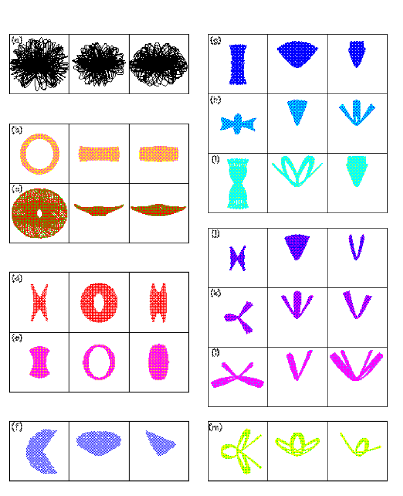
Figure 1:

Major families of orbits in triaxial black-hole nuclei. Each set of three frames shows, from left to right, projections onto the ($x,y$), ($y,z$) and ($x,z$) planes. (a) Stochastic orbit. (b) Short-axis tube orbit. (c) Saucer orbit, a resonant short-axis tube. (d) Inner long-axis tube orbit. (e) Outer long-axis tube orbit. (f) ($1,-2,1)$ resonant orbit. (g) Pyramid orbit. (h) ($3,0,-4$) resonant pyramid orbit. (i) ($0,6,-5$) resonant pyramid orbit. (j) Banana orbit. (k) $2:3:4$ resonant banana orbit. (l) $3:4:6$ resonant banana orbit. (m) $6:7:8$ resonant orbit.

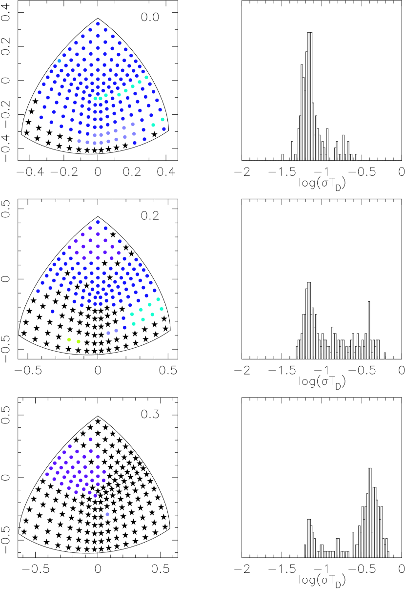
Figure 2:

Stationary start space for mass model with $\gamma=1$ (weak cusp) and $T=c/a=0.5$. Left panels show initial positions on one octant of the equipotential surface; $x$ axis is toward the lower left and $z$ axis is up. Frames are labelled by $\log\left(M_{*}/M_{\bullet}\right)$. Circles represent starting points of regular orbits and stars represent stochastic orbits. Colors match the colors of the orbit families in Figure 1. Right panels show histograms of Liapunov exponents computed over 100 dynamical times.

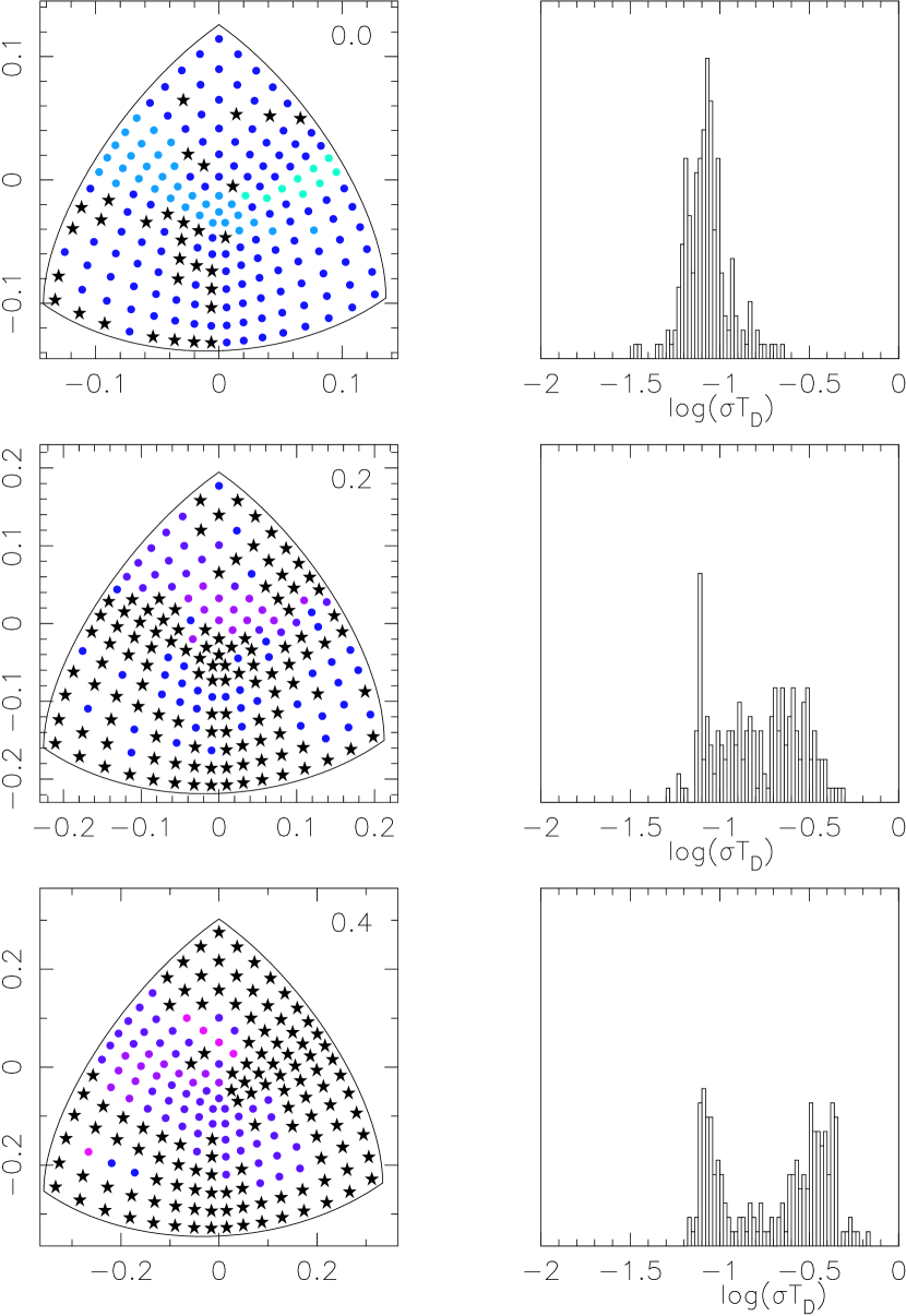
Figure 3:

Like Figure 2, for $\gamma=2$ (strong cusp). As in the weak-cusp case, pyramid orbits dominate at low energies and bananas at high energies.

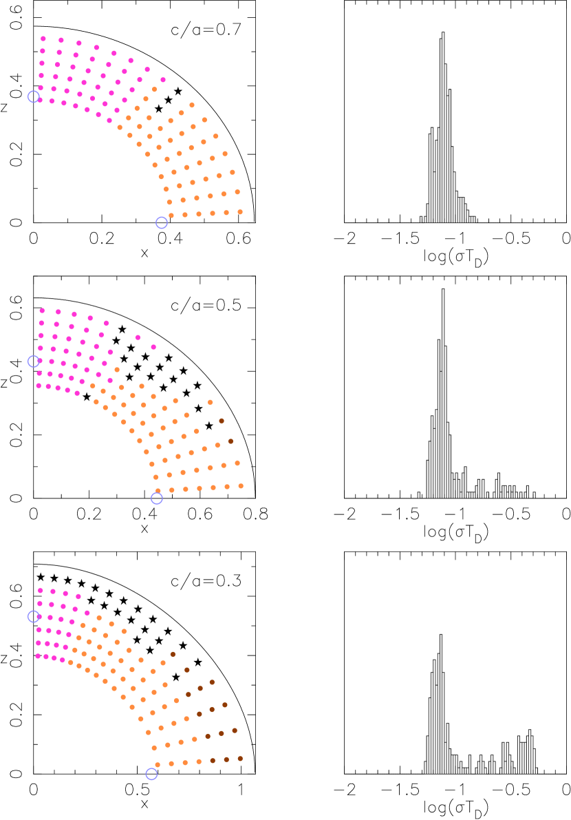
Figure 4:

$X-Z$ start space for mass models with $\gamma=1$ (weak cusp), $T=0.5$ and three values of $c/a$. Energy is fixed to that of the shell with $\log\left(M_{*}/M_{\bullet}\right)=0.2$. Left panels show initial positions in the ($x,z$) plane. Circles represent starting points of regular orbits and stars represent stochastic orbits. Colors match the colors of the orbit families in Figure 1. Open circles mark the $1:1$ closed orbits in the principal planes. Right panels show histograms of Liapunov exponents computed over 100 dynamical times. As the elongation of the model is increased, stochastic and resonant orbits (e.g. the saucers) become more prominent.

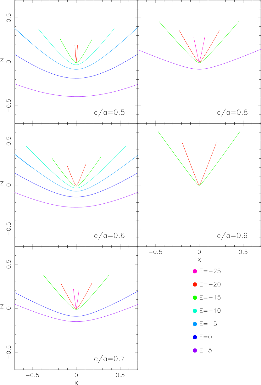
Figure 5:

Banana orbits as a function of energy in five models, each with $\gamma=2$ and $T=0.5$. Unstable bananas are not shown.

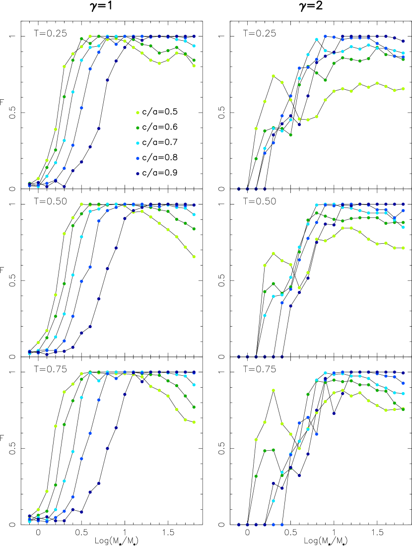
Figure 6:

Fraction of chaotic orbits in stationary start space for $\gamma=1$ (weak cusp) and $\gamma=2$ (strong cusp) models as a function of energy.

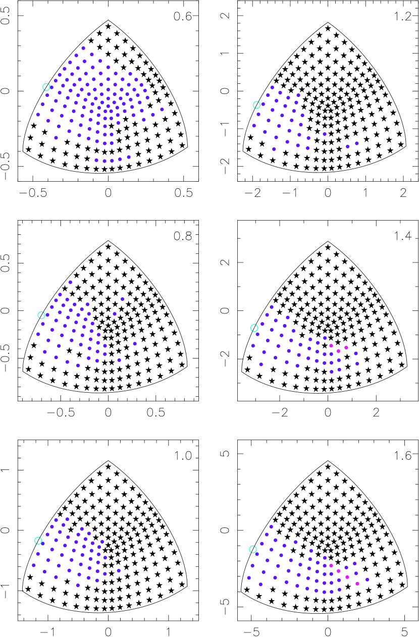
Figure 7:

Stationary start space for the model with $\gamma=2,T=c/a=0.5$ as a function of energy, through the “zone of chaos.” The banana family of orbits persists throughout the chaotic zone. The starting points of the resonant banana orbits are shown by the open circles.

References

- Bender & Saglia (1999) Bender, R. & Saglia, R. 1999, in Galaxy Dynamics, ASP Conf. Ser. 182, ed. D. Merritt, J. A. Sellwood & M. Valluri (ASP: Provo), 113
- Carlson (1988) Carlson, B. C. 1988, A Table of Elliptic Integrals of the Third Kind. Mathematics of Computation, Vol. 51, No. 183, 267
- Carpintero & Aguilar (1998) Carpintero, D. D. & Aguilar, L. A. 1998, MNRAS, 298, 1
- Chandrasekhar (1969) Chandrasekhar, S. 1969, Ellipsoidal Figures of Equilibrium [Dover: New York]
- Crane et al. (1993) Crane, P. et al. 1993, AJ, 106, 1371
- Dehnen (1993) Dehnen, W. 1993, MNRAS, 265, 250
- de Zeeuw (1985) de Zeeuw, P. T. 1985, MNRAS, 216, 273
- de Zeeuw & Pfenniger (1988) de Zeeuw, P. T. & Pfenniger, D. 1988, MNRAS, 235, 949
- Ebisuzaki, Makino & Okumura (1991) Ebisuzaki, T., Makino, J. & Okumura, S. K. 1991, Nature, 354, 212
- Ferrarese et al. (1994) Ferrarese, L., van den Bosch, F. C., Ford, H. C., Jaffe, W. & O’Connell, R. W. 1994, AJ, 108, 1598
- Ford et al. (1998) Ford, H. C., Tsvetanov, Z. I., Ferrarese, L. & Jaffe, W. 1998, in IAU Symp. 184, The Central Regions of the Galaxy and Galaxies, ed. Y. Sofue (Dordrecht: Kluwer), 377
- Gebhardt et al. (1996) Gebhardt, K. et al. 1996, AJ, 112, 105
- Gebhardt et al. (2000) Gebhardt, K. et al. 2000, AJ, 119, 1157
- Gerhard & Binney (1985) Gerhard, O. E. & Binney, J. 1985, MNRAS, 216, 467
- Goodman & Schwarzschild (1981) Goodman, J. & Schwarzschild, M. 1981, ApJ, 245, 1087
- Hairer & Wanner (1996) Hairer, E. & Wanner, G. 1996, Solving Ordinary Differential Equations. II. [Berlin: Springer]
- Kormendy (1985) Kormendy, J. 1985, ApJ, 292, L9
- Lees & Schwarzschild (1992) Lees, J. F. & Schwarzschild, M. 1992, ApJ, 384, 491
- Macchetto et al. (1997) Macchetto, F. et al. 1997, ApJ, 489, 579
- Makino (1997) Makino, J. 1997, ApJ, 478, 58
- Merritt (1999) Merritt, D. 1999, in Galaxy Dynamics, ASP Conf. Ser. 182, ed. D. Merritt, J. A. Sellwood & M. Valluri (ASP: Provo), 164
- Merritt & Fridman (1995) Merritt, D. & Fridman, T. 1995, in Fresh Views of Elliptical Galaxies, ASP Conf. Ser. 86, ed. A. Buzzoni, A. Renzini & A. Serrano (ASP: Provo), 13
- Merritt & Fridman (1996) Merritt, D. & Fridman, T. 1996, ApJ, 460, 136
- Merritt & Valluri (1996) Merritt, D. & Valluri, M. 1996, ApJ, 471, 82
- Merritt & Valluri (1999) Merritt, D. & Valluri, M. 1999, AJ, 118, 1177
- Papaphilippou & Laskar (1998) Papaphilippou, Y. & Laskar, J. 1998, A& A, 329, 451
- Peebles (1972) Peebles, P. J. E. 1972, Gen. Rel. Grav., 3, 63
- Quillen (1999) Quillen, A. C. 1999, in Galaxy Dynamics, ASP Conf. Ser. 182, ed. D. Merritt, J. A. Sellwood & M. Valluri (ASP: Provo), 138
- Quinlan & Hernquist (1997) Quinlan, G. & Hernquist, L. 1997, New A, 2, 533
- Quinlan, Hernquist & Sigurdsson (1995) Quinlan, G., Hernquist, L. & Sigurdsson, S. 1995, ApJ, 440, 554
- Ryden (1999) Ryden, B. 1999, in Galaxy Dynamics, ASP Conf. Ser. 182, ed. D. Merritt, J. A. Sellwood & M. Valluri (ASP: Provo), 142
- Schwarzschild (1993) Schwarzschild, M. 1993, ApJ, 409, 563
- Sridhar & Touma (1999) Sridhar, S. & Touma, J. 1999, MNRAS, 303, 483
- Sambhus & Sridhar (2000) Sambhus, N. & Sridhar, S. 2000, preprint
- van der Marel (1994) van der Marel, R. 1994, MNRAS, 270, 271
- Valluri & Merritt (1998) Vallrui, M. & Merritt, D. 1998, ApJ, 506, 686
- Wachlin & Ferraz-Mello (1998) Wachlin, F. C. & Ferraz-Mello, S. 1998, MNRAS, 298, 22