OUT OF EQUILIBRIUM FIELDS IN SELFCONSISTENT INFLATIONARY DYNAMICS. DENSITY FLUCTUATIONS

Abstract

The physics during the inflationary stage of the universe is of quantum nature involving extremely high energy densities. Moreover, it is out of equilibrium on a fastly expanding dynamical geometry. We present in these lectures non-perturbative out of equilibrium field theoretical methods in cosmological universes. We then study the non-linear dynamics of quantum fields in matter and radiation dominated FRW and de Sitter universes. For a variety of initial conditions, we compute the evolution of the quantum inflaton field, its large quantum fluctuations and the equation of state. We investigate the explosive particle production due to spinodal instabilities and parametric amplification in FRW and de Sitter universes with and without symmetry breaking. We show how the particle production is sensitive to the expansion of the universe. In the large $N$ limit for symmetry breaking scenarios, we determine generic late time fields behavior for any flat FRW and de Sitter cosmology. We show that the amplitude of the quantum fluctuations fall off in FRW with the square of the scale factor while the order parameter approaches a minimum of the potential in the same manner. We present a complete and numerically accessible renormalization scheme for the equation of motion and the energy momentum tensor in flat cosmologies. Furthermore, we consider an $O(N)$ inflaton model coupled self-consistently to gravity in the semiclassical approximation, where the field is subject to ‘new inflation’ type initial conditions. We study the dynamics self-consistently and non-perturbatively with non-equilibrium field theory methods in the large $N$ limit. We find that spinodal instabilities drive the growth of non-perturbatively large quantum fluctuations which shut off the inflationary growth of the scale factor. We find that a very specific combination of these large quantum fluctuations plus the inflaton zero mode assemble into a new effective field. This new field behaves classically and it is the object which actually rolls down. The metric perturbations during inflation are computed using this effective field and the Bardeen variable for superhorizon modes during inflation. We compute the amplitude and index for the spectrum of scalar density and tensor perturbations and argue that in all models of this type the spinodal instabilities are responsible for a ‘red’ spectrum of primordial scalar density perturbations.

I Introduction and Motivation

Inflationary cosmology has come of age. From its beginnings as a solution to the horizon, flatness, entropy and monopole problems[2], it has grown into the main contender for the explanation of the source of primordial fluctuations giving rise to large scale structure[27]. There is evidence from the measurements of temperature anisotropies in the cosmic microwave background radiation (CMBR) that the scale invariant power spectrum predicted by generic inflationary models is consistent with observations[3, 4, 5] and we can expect further and more exacting tests of the predictions of inflation when the MAP and PLANCK missions are flown. In particular, if the fluctuations that are responsible for the temperature anisotropies of the CMB truly originate from quantum fluctuations during inflation, determinations of the spectrum of scalar and tensor perturbations will constrain inflationary models based on particle physics scenarios and probably will validate or rule out specific proposals[4, 28].

The tasks for inflationary universe researchers are then two-fold. First, models of inflation must be constructed on the basis of a realistic particle physics model. This is in contrast to the current situation where most, if not all acceptable inflationary models are ad-hoc in nature, with fields and potentials put in for the sole purpose of generating an inflationary epoch. Second, and equally important, the quantum dynamics of inflation must be understood. This is extremely important, especially in light of the fact that it is exactly this quantum behavior that is supposed to give rise to the primordial metric perturbations which presumably have imprinted themselves in the CMBR. This latter problem is the focus of this review.

The inflaton must be treated as a non-equilibrium quantum field . The simplest way to see this comes from the requirement of having small enough metric perturbation amplitudes which in turn requires that the quartic self coupling $\lambda$ of the inflaton be extremely small, typically of order $\sim 10^{-12}$. Such a small coupling cannot establish local thermodynamic equilibrium (LTE) for all field modes; typically the long wavelength modes will respond too slowly to be able to enter LTE. In fact, the superhorizon sized modes will be out of the region of causal contact and cannot thermalize. We see then that if we want to gain a deeper understanding of inflation, non-equilibrium tools must be developed. Such tools exist and have now been developed to the point that they can give quantitative answers to these questions in cosmology[8] -[17],[20, 21, 33, 34]. These methods permit us to follow the dynamics of quantum fields in situations where the energy density is non-perturbatively large ($\sim 1/\lambda$). That is, they allow the computation of the time evolution of non-stationary states and of non-thermal density matrices.

Our programme on non-equilibrium dynamics of quantum field theory, started in 1992[8], is naturally poised to provide a framework to study these problems. The larger goal of the program is to study the dynamics of non-equilibrium processes from a fundamental field-theoretical description, by solving the dynamical equations of motion of the underlying four dimensional quantum field theory for physically relevant problems: the early universe dynamics, high energy particle collisions, phase transitions out of equilibrium, symmetry breaking and dissipative processes.

The focus of our work is to describe the quantum field dynamics when the energy density is high. That is, a large number of particles per volume $m^{-3}$, where $m$ is the typical mass scale in the theory. Usual S-matrix calculations apply in the opposite limit of low energy density and since they only provide information on in $\rightarrow$ out matrix elements, are unsuitable for calculations of expectation values.

In high energy density situations such as in the early universe, the particle propagator (or Green function) depends on the particle distribution in momenta in a nontrivial way. This makes the quantum dynamics intrinsically nonlinear and calls to the use of self-consistent non-perturbative approaches as the large $N$ limit, Hartree and self-consistent one-loop approximations.

There are basically three different levels to study the early universe dynamics:

1. To work out the nonlinear dynamics of quantum fields in Minkowski spacetime. By non-linear dynamics we understand to solve the quantum equations of motion including the quantum back-reaction quantitatively[8] -[10], [19, 25, 33, 34]. This level is in fact appropriate to describe high energy particle collisions [36].

2. To work out the nonlinear dynamics of quantum fields in fixed cosmological backgrounds[13, 14]. New phenomena arise then compared with 1. showing that a Minkowski analysis is not quantitatively precise for expanding universes.

3. A self-consistent treatment of the quantum fields and the cosmological background[15, 35]. That is, the metric is obtained dynamically from the quantum fields (matter source) propagating in the that metric.

We shall successively present the three levels of study. The first stage was reviewed in the 1996 Chalonge School [10]. The second level is the subject of secs. VI and VII. We study the parametric and spinodal resonances both in FRW and de Sitter backgrounds wide range of initial conditions both in FRW and de Sitter backgrounds [12, 14]. [Parametric resonance appears in chaotic inflationary scenarios for unbroken symmetry whereas spinodal unstabilities show up in new inflation scenarios with broken symmetry]. Both types of unstabilities shut-off through the non-linear quantum evolution as described in secs. VI and VII [12, 14] both analytically and numerically. We follow the equation of state of the quantum matter during the evolution and analyze its properties.

The third stage of our approach is to apply non-equilibrium quantum field theory techniques to the situation of a scalar field coupled to semiclassical gravity, where the source of the gravitational field is the expectation value of the stress energy tensor in the relevant, dynamically changing, quantum state. In this way we can go beyond the standard analyses[29, 30, 31, 32] which treat the background as fixed and do not consider the non-linear quantum field dynamics.

In all cases 1. - 3. , the quantum fields energy- momentum tensor is covariantly conserved both at the regularized as well as the renormalized levels [9] - [15].

We mainly consider for the stage 3. new inflation scenarios where a scalar field $\phi$ evolves under the action of a typical symmetry breaking potential. The initial conditions will be taken so that the initial value of the order parameter is near the top of the potential (the disordered state) with essentially zero time derivative. What we find is that the existence of spinodal instabilities, i.e. the fact that eventually (in an expanding universe) all modes will act as if they have a negative mass squared, drives the quantum fluctuations to grow non-perturbatively large. We have the picture of an initial wave-function or density matrix peaked near the unstable state and then spreading until it samples the stable vacua. Since these vacua are non-perturbatively far from the initial state (typically $\sim m/\sqrt{\lambda}$, where $m$ is the mass scale of the field and $\lambda$ the quartic self-coupling), the spinodal instabilities will persist until the quantum fluctuations, as encoded in the equal time two-point function $\langle\Phi(\vec{x},t)^{2}\rangle$, grow to ${\cal O}(m^{2}/\lambda$).

This growth eventually shuts off the inflationary behavior of the scale factor as well as the growth of the quantum fluctuations (this last also happens in Minkowski spacetime [9, 10]).

The scenario envisaged here is that of a quenched or super-cooled phase transition where the order parameter is zero or very small. Therefore one is led to ask:

a) What is rolling down?.

b) Since the quantum fluctuations are non-perturbatively large ( $\sim 1/\lambda$), will not they modify drastically the FRW dynamics?.

c) How can one extract (small?) metric perturbations from non-perturbatively large field fluctuations?

We address the questions a)-c) as well as other issues in sec. IX.

We choose such type of new inflationary scenario because the issue of large quantum fluctuations is particularly dramatic there. However, our methods do apply to any inflationary scenario as chaotic, extended and hybrid inflation.

II Non-Equilibrium Quantum Field Theory, Semiclassical Gravity and Inflation

We present here the framework of the non-equilibrium closed time path formalism. For a more complete discussion, the reader is referred to [9]-[16].

The time evolution of a system is determined in the Schrödinger picture by the functional Liouville equation

$$i\frac{\partial\rho(t)}{\partial t}=[H(t),\rho(t)],$$ (1)

where $\rho$ is the density matrix and we allow for an explicitly time dependent Hamiltonian as is necessary to treat quantum fields in a time dependent background. Formally, the solutions to this equation for the time evolving density matrix are given by the time evolution operator, $U(t,t^{{}^{\prime}})$, in the form

$$\rho(t)=U(t,t_{0})\rho(t_{0})U^{-1}(t,t_{0}).$$ (2)

The quantity $\rho(t_{0})$ determines the initial condition for the evolution. We choose this initial condition to describe a state of local equilibrium in conformal time, which is also identified with the conformal adiabatic vacuum for short wavelengths.

Given the evolution of the density matrix (2), ensemble averages of operators are given by the expression (again in the Schrödinger picture)

$$\langle{\cal O}(t)\rangle=\frac{Tr[U(t_{0},t){\cal O}U(t,t^{{}^{\prime}})U(t^{{}^{\prime}},t_{0})\rho(t_{0})]}{Tr\rho(t_{0})},$$ (3)

where we have inserted the identity, $U(t,t^{{}^{\prime}})U(t^{{}^{\prime}},t)$ with $t^{{}^{\prime}}$ an arbitrary time which will be taken to infinity. The state is first evolved forward from the initial time $t_{0}$ to $t$ when the operator is inserted. We then evolve this state forward to time $t^{{}^{\prime}}$ and back again to the initial time[9, 12].

We shall study the inflationary dynamics in a spatially flat Friedmann-Robertson-Walker background with scale factor $a(t)$ and line element:

$$ds^{2}=dt^{2}-a^{2}(t)\;d\vec{x}^{2}.$$ (4)

Our Lagrangian density has the form

$${\cal L}=\sqrt{-g}\left[\frac{1}{2}\nabla_{\mu}\Phi\nabla^{\mu}\Phi-V(\Phi)\right]\;.$$ (5)

Our approach can be generalized to open as well as closed cosmologies.

Our program incorporates the non-equilibrium behavior of the quantum fields involved in inflation into a framework where the geometry (gravity) is dynamical and is treated self consistently. We do this via the use of semiclassical gravity[24] where we say that the metric is classical and determined through the Einstein equations using the expectation value of the stress energy tensor $\langle T_{\mu\nu}\rangle$. Such expectation value is taken in the dynamically determined state described by the density matrix $\rho(t)$. This dynamical problem can be described schematically as follows:

1. The dynamics of the scale factor $a(t)$ is driven by the semiclassical Einstein equations

   $$\frac{1}{8\pi G_{R}}G_{\mu\nu}+\frac{\Lambda_{R}}{8\pi G_{R}}\;g_{\mu\nu}+\left(\rm{higher\ curvature}\right)=-\langle T_{\mu\nu}\rangle_{R}.$$ (6)

   Here $G_{R},\Lambda_{R}$ are the renormalized values of Newton’s constant and the cosmological constant, respectively and $G_{\mu\nu}$ is the Einstein tensor. The higher curvature terms must be included to absorb ultraviolet divergences.

2. On the other hand, the density matrix $\rho(t)$ of the matter (that determines $\langle T_{\mu\nu}\rangle_{R}$) obeys the Liouville equation (1) with $H$ is the evolution Hamiltonian, which is dependent on the scale factor, $a(t)$.

It is this set of equations we must try to solve specifying the appropriate initial conditions.

A On the initial state: dynamics of phase transitions

The situations we consider are

1. the theory admits a symmetry breaking potential and in which the field expectation value starts its evolution near the unstable point.

2. The symmetry is not broken and the field expectation value starts its evolution at a finite distance from the absolute minimum.

There is an issue as to how the field got to have an expectation value near the unstable point (typically at $\Phi=0$) as well as an issue concerning the initial state of the non-zero momentum modes.

Since our background is an FRW spacetime, it is spatially homogeneous and we can choose our state $\rho(t)$ to respect this symmetry. Starting from the full quantum field $\Phi(\vec{x},t)$ we can extract its expectation value $\phi(t)$ by writing:

$$\Phi(\vec{x},t)=\phi(t)+\Psi(\vec{x},t)\quad,\quad\phi(t)={\rm Tr}[\rho(t)\Phi(\vec{x},t)]\equiv\langle\Phi(\vec{x},t))\rangle.$$ (7)

The quantity $\Psi(\vec{x},t)$ represents the quantum fluctuations about the zero mode $\phi(t)$ and clearly satisfies $\langle\Psi(\vec{x},t)\rangle=0$.

We need to choose a basis to represent the density matrix. A natural choice consistent with the translational invariance of our quantum state is that given by the Fourier modes, in comoving momentum space, of the quantum fluctuations $\Psi(\vec{x},t)$:

$$\Psi(\vec{x},t)=\int\frac{d^{3}k}{(2\pi)^{3}}\;\exp(-i\ \vec{k}\cdot\vec{x})\;\psi_{k}(t).$$ (8)

In this language we can state our ansatz for the initial condition of the quantum state as follows. We take the zero mode $\phi(t=0)=\phi_{0},\ \dot{\phi}(t=0)=0$, where $\phi_{0}$ will typically be very near the origin for broken symmetry and at a finite distance from it in the unbroken symmetry case. The initial conditions on the the nonzero modes $\psi_{k}(t)$ will be chosen such that the initial density matrix $\rho(t=0)$ describes a vacuum state (i.e. an initial state in local thermal equilibrium at a temperature $T_{i}=0$). There are some subtleties involved in this choice. First, as explained in [13], in order for the density matrix to commute with the initial Hamiltonian, we must choose the modes to be initially in the conformal adiabatic vacuum (these statements will be made more precise below). This choice has the added benefit of allowing for time independent renormalization counterterms to be used in renormalizing the theory.

We are making the assumption of an initial vacuum state in order to be able to proceed with the calculation. It would be interesting to understand what forms of the density matrix can be used for other more general initial conditions[46].

The assumptions of an initial equilibrium vacuum state are essentially the same used in refs. [29], [30] and [32] in the analysis of the quantum mechanics of inflation in a fixed de Sitter background.

As discussed in the introduction, if we start from such an initial state, spinodal or parametric instabilities will drive the growth of non-perturbatively large quantum fluctuations. In order to deal with these, we need to be able to perform calculations that take these large fluctuations into account. Although the quantitative features of the dynamics will depend on the initial state, the qualitative features associated with spinodal or parametric unstabilities are fairly robust for a wide choice of initial states that describe a phase transition.

III The Inflaton Model and the Equations of Motion

Having recognized the appearance of large quantum fluctuations driven by parametric or spinodal unstabilities, we need to study the dynamics within a non-perturbative framework. That is, a framework allowing calculations for non-perturbatively large energy densities. We require that such a framework be: i) renormalizable, ii) covariant energy conserving, iii) numerically implementable. There are very few schemes that fulfill all of these criteria: the large $N$ and the Hartree approximation[9]-[15]. Whereas the Hartree approximation is basically a Gaussian variational approximation[23] that in general cannot be consistently improved upon, the large $N$ approximation can be consistently implemented beyond leading order[33, 34]. In addition, the presence of a large number of fields in most of the GUT’s models suggest that the large $N$ limit will be actually a realistic one. Moreover, for the case of broken symmetry it has the added bonus of providing many light fields (associated with Goldstone modes) that will permit the study of the effects of other fields which are lighter than the inflaton on the dynamics. Thus we will study the inflationary dynamics within the framework of the large $N$ limit of a scalar theory in the vector representation of $O(N)$ both for unbroken and broken symmetry. In the second case we will have a quenched phase transition.

We assume that the universe is spatially flat with a metric given by eq.(4). The matter action and Lagrangian density are given by eq.(5),

$$S_{m}=\int d^{4}x\;{\cal L}_{m}=\int d^{4}x\;a^{3}(t)\left[\frac{1}{2}\dot{\vec{\Phi}}^{2}(x)-\frac{1}{2}\frac{(\vec{\nabla}\vec{\Phi}(x))^{2}}{a^{2}(t)}-V(\vec{\Phi}(x))\right]$$ (9)

$$V(\vec{\Phi})=\frac{m^{2}}{2}\;\vec{\Phi}^{2}+\frac{\lambda}{8N}\left(\vec{\Phi}^{2}+\frac{2Nm^{2}}{\lambda}\right)^{2}+\frac{1}{2}\,\xi\;{\cal R}\;\vec{\Phi}^{2}\;,$$ (10)

where $m^{2}>0$ for unbroken symmetry and $m^{2}<0$ for broken symmetry. Here ${\cal R}(t)$ stands for the scalar curvature

$${\cal R}(t)=6\left(\frac{\ddot{a}(t)}{a(t)}+\frac{\dot{a}^{2}(t)}{a^{2}(t)}\right),$$ (11)

The $\xi$-coupling of $\vec{\Phi(x)}^{2}$ to the scalar curvature ${\cal R}(t)$ has been included since arises anyhow as a consequence of renormalization[12].

The gravitational sector includes the usual Einstein term in addition to a higher order curvature term and a cosmological constant term which are necessary to renormalize the theory. The action for the gravitational sector is therefore:

$$S_{g}=\int d^{4}x\;{\cal L}_{g}=\int d^{4}x\,a^{3}(t)\left[\frac{{\cal R}(t)}{16\pi G}+\frac{\alpha}{2}\;{\cal R}^{2}(t)-K\right].$$ (12)

with $K$ being the cosmological constant. In principle, we also need to include the terms $R^{\mu\nu}R_{\mu\nu}$ and $R^{\alpha\beta\mu\nu}R_{\alpha\beta\mu\nu}$ as they are also terms of fourth order in derivatives of the metric (fourth adiabatic order), but the variations resulting from these terms turn out not to be independent of that of ${\cal R}^{2}$ in the flat FRW cosmology we are considering.

The variation of the action $S=S_{g}+S_{m}$ with respect to the metric $g_{\mu\nu}$ gives us Einstein’s equation

$$\frac{G_{\mu\nu}}{8\pi G}+\alpha\;H_{\mu\nu}+K\;g_{\mu\nu}=-<T_{\mu\nu}>\;,$$ (13)

where $G_{\mu\nu}$ is the Einstein tensor given by the variation of $\sqrt{-g}{\cal R}$, $H_{\mu\nu}$ is the higher order curvature term given by the variation of $\sqrt{-g}{\cal R}^{2}$, and $T_{\mu\nu}$ is the contribution from the matter Lagrangian. With the metric (4), the various components of the curvature tensors in terms of the scale factor are:

$$G^{0}_{0} = -3\,\left({\dot{a}\over a}\right)^{2}\;,\;G^{\mu}_{\mu}=-{\cal R}=-6\left(\frac{\ddot{a}}{a}+\frac{\dot{a}^{2}}{a^{2}}\right)\;,$$ (14)

$$H^{0}_{0} = -6\left(\frac{\dot{a}}{a}\;\dot{{\cal R}}+\frac{\dot{a}^{2}}{a^{2}}\;{\cal R}-\frac{1}{12}\;{\cal R}^{2}\right)\;,\;H^{\mu}_{\mu}=-6\left(\ddot{{\cal R}}+3\;\frac{\dot{a}}{a}\;\dot{{\cal R}}\right)\;.$$ (15)

Eventually, when we have fully renormalized the theory, we will set $\alpha_{R}=0$ and keep as our only contribution to $K_{R}$ a piece related to the matter fields which we shall incorporate into $T_{\mu\nu}$.

The use of semiclassical gravity (i. e. neglecting graviton loops) is justified since graviton loops are suppressed by factors $(m/M_{Pl})^{2}$ where $m$ is at the GUT scale and hence $(m/M_{Pl})^{2}\sim 10^{-8}$.

IV The Large N Limit for a scalar field with an arbitrary invariant self-interaction

We present here the systematic derivation of the $1/N$ expansion for the scalar model with an arbitrary $O(N)$-invariant self-interaction and the scalar field in the vector representation of $O(N)$[44]-[45]. We consider Minkowski space-time. The generalization to the cosmological space-time (4) is discussed at the end of the section.

The action and Lagrangian density are given by,

$$S=\int d^{4}x\;{\cal L}\quad,\quad{\cal L}=\frac{1}{2}\left[\partial{\vec{\Phi}}(x)\right]^{2}-N\,V\left(\frac{1}{N}\;\vec{\Phi}^{2}(x)\right)\;.$$ (16)

This choice of the $N$ dependence in the interaction ensures that the large $N$ limit exists. In particular, for a quartic potential we choose according to eq.(10):

$$V\left(\frac{1}{N}\;\vec{\Phi}^{2}(x)\right)=\frac{\lambda}{8N^{2}}\left(\vec{\Phi}^{2}+\frac{2Nm^{2}}{\lambda}\right)^{2}\quad.$$ (17)

The functional integral for the model takes the form

$${\cal Z}[J(.)]=\int\int D\vec{\Phi}\;\exp{i\int d^{4}x\left[{\cal L}+{\vec{\Phi}}(x).{\vec{J}}(x)\right]}$$ (18)

where ${\vec{J}}(x)$ is an external source introduced to generate the correlation functions. For example, the connected two point correlation function is expressed as

$$<T\Phi_{i}(x)\,\Phi_{k}(y)>=i^{-2}\;\left.{{\delta^{2}}\over{\delta J_{i}(x)\,\delta J_{k}(y)}}\log{\cal Z}[J(.)]\right|_{J_{i}(.)=0}\;.$$ (19)

In order to compute the large $N$ limit it is convenient to replace the interaction term by the following functional integral representation [45]:

$$\exp{-iN\int d^{4}x\;V(\frac{1}{N}\vec{\Phi}^{2}(x))} = \int\int Dz\;\Pi_{x}\,\delta\left(z(x)-\frac{1}{N}\vec{\Phi}^{2}(x)\right)\;e^{-iN\int d^{4}x\,V(z(x))}$$ (20)

$$= \int\int Dz\;D\sigma\;e^{iN\int d^{4}x\,\left[\frac{1}{2}\sigma(x)\,\left(z(x)-\frac{1}{N}\vec{\Phi}^{2}(x)\right)-V(z(x))\right]}$$ (22)

Inserting eq.(20) into eq.(18), the integration over $\vec{\Phi}(x)$ becomes gaussian and therefore can be exactly computed with the result:

$${\cal Z}[J(.)]=\int\int D\vec{\Phi}\;Dz\;D\sigma\;e^{i\int d^{4}x\left[\frac{1}{2}\left[\partial{\vec{\Phi}}(x)\right]^{2}+\frac{N}{2}\sigma(x)\,z(x)-\frac{1}{2}\sigma(x)\,\vec{\Phi}^{2}(x)-N\,V(z(x))+{\vec{\Phi}}(x).{\vec{J}}(x)\right]}$$ (23)

(24)

$$=\int\int Dz\;D\sigma\;\left\{\det\left[\partial^{2}+\sigma(.)\right]\right\}^{-\frac{N}{2}}\;e^{iN\int d^{4}x\left[\frac{1}{2}\sigma(x)\,z(x)-V(z(x))\right]+\frac{i}{2}\int d^{4}x\;d^{4}y\;J_{i}(x)\;G(x,y,\sigma(.))\;J_{i}(y)}$$ (25)

Here, $G(x,y,\sigma(.))$ is the inverse operator of $\partial^{2}+\sigma(.)$. That is,

$$\left[\partial^{2}+\sigma(x)\right]G(x,y,\sigma(.))=\delta(x-y)$$ (26)

It is useful to introduce a source $N\,K(x)$ for the field $z(x)$. This will permit to generate the correlation functions of the composite field $\vec{\Phi}^{2}(x)$. The generating functional now takes the form

$${\cal Z}[J(.),K(.)]=\int\int Dz\;D\sigma\;\left\{\det\left[\partial^{2}+\sigma(.)\right]\right\}^{-\frac{N}{2}}\;e^{iN\int d^{4}x\left[\frac{1}{2}\sigma(x)\,z(x)-V(z(x))\right]}$$ (27)

(28)

$$e^{\frac{i}{2}\int d^{4}x\;d^{4}y\;J_{i}(x)\;G(x,y,\sigma(.))\;J_{i}(y)+iN\int d^{4}x\;K(x)\;z(x)}=\int\int Dz\;D\sigma\;e^{iN{\cal S}[z(.),\sigma(.)]}\;.$$ (29)

Here,

$${\cal S}[z(.),\sigma(.)] = \frac{i}{2}\log\det\left[\partial^{2}+\sigma(.)\right]+\int d^{4}x\left[\frac{1}{2}\sigma(x)\,z(x)-V(z(x))+K(x)\;z(x)\right]$$ (30)

$$+ \frac{1}{2N}\int d^{4}x\;d^{4}y\;G(x,y,\sigma(.))\;J_{i}(x)\;J_{i}(y)\;.$$ (32)

Notice that the source terms in ${\cal S}$ are both of order one since $K(x)$ and $J_{i}(x)$ are assumed to be of order one.

The functional derivatives with respect to the source $K(x)$ at $K(x)=0$ produce the insertions

$${1\over i}{{\delta}\over{\delta K(x)}}\Rightarrow N\,z(x)=\vec{\Phi}^{2}(x)\;.$$ (33)

as follows from eqs.(20) and (27) That is, $K(x)$ is the source of the composite field $\vec{\Phi}^{2}(x)$. The correlations of $\vec{\Phi}^{2}(x)$ follow as functional derivatives of $\log{\cal Z}[J(.),K(.)]$ with respect to $K(x)$. For example, we have for the two points function

$$<T\,\vec{\Phi}^{2}(x)\,\vec{\Phi}^{2}(y)>=i^{-2}\;\left.{{\delta^{2}}\over{\delta K(x)\,\delta K(y)}}\log{\cal Z}[J(.),K(.)]\right|_{J(.)=,K(.)=0}\;.$$

Since in eq.(27) the $N$-dependence is explicit in the exponent, we can take the large $N$ limit by looking for the stationary points of the action there.

Extremizing ${\cal S}[z(.),\sigma(.)]$ with respect to the field $\sigma(x)$ yields:

$$i\,G(x,x,\sigma(.))+z(x)-\frac{1}{N}\,\left[\int d^{4}y\;G(x,y,\sigma(.))\,J_{i}(y)\right]^{2}=0$$ (34)

Where we used that,

$${{\delta G(y,z,\sigma(.))}\over{\delta\sigma(x)}}=-G(y,x,\sigma(.))\;G(x,z,\sigma(.))\;.$$ (35)

Eq.(35) can be derived as follows. Taking the functional derivative of eq.(26) with respect to $\sigma(.)$ yields,

$$\left[\partial^{2}+\sigma(x)\right]{{\delta G(x,y,\sigma(.))}\over{\delta\sigma(z)}}=-\delta(x-z)G(x,y,\sigma(.))$$

This is an equation for ${{\delta G(x,y,\sigma(.))}\over{\delta\sigma(z)}}$ that can be solved using the inverse operator of $\left[\partial^{2}+\sigma(x)\right]$ as given by eq.(26). This gives eq.(35).

Extremizing ${\cal S}[z(.),\sigma(.)]$ with respect to the field $z(x)$ yields:

$$\frac{1}{2}\sigma(x)-V^{\prime}\left(z(x)\right)+K(x)=0\;.$$ (36)

Eqs.(34)-(36) define the saddle point $\sigma(x),z(x)$ as a functional of the sources $J(.),K(.)$. One has thus to make the following shift of the functional integration variables

$$\sigma(x)=\sigma(x)+\xi(x)\;,\;z(x)=z(x)+w(x)$$ (37)

where $\xi(x),w(x)$ are the new functional integration variables.

Now we have to insert the change (37) into eq.(30) and expand ${\cal S}[z(.),\sigma(.)]$ in powers of $\xi(x)$ and $w(x)$. The zeroth order, that is ${\cal S}[z(.),\sigma(.)]$ yields the $N=\infty$ limit of the model. The quadratic part in $\xi(x)$ and $w(x)$ provides the propagators and the higher orders provide the vertices of the $1/N$ perturbation theory.

A The Large $N$ Limit for the $[\vec{\Phi}^{2}]^{2}$ theory

For simplicity, we will restrict ourselves to the $\Phi^{4}$ theory with potential (17). That is,

$$V(z)=\frac{\lambda}{8}\left(z+\frac{2m^{2}}{\lambda}\right)^{2}=\frac{\lambda}{8}\,z^{2}+\frac{m^{2}}{2}\,z+{{m^{4}}\over{2\lambda}}\quad.$$ (38)

In this important case we have $V^{\prime}(z)=\frac{\lambda\;z}{4}+\frac{m^{2}}{2}$ and we can eliminate $z(x)$ using the saddle point equation (36),

$$z(x)=\frac{2}{\lambda}\left[\sigma(x)+2K(x)-m^{2}\right]\;.$$ (39)

Equivalently, in this case we can integrate exactly over $z(x)$ in eqs.(20), (23) and (27) since these functional integrals become gaussian in the field $z$ when $V(z)$ is given by eq.(38).

The saddle point equation (34) for $\sigma(x)$ becomes

$$i\,G(x,x,\sigma(.))+\frac{2}{\lambda}\left[\sigma(x)+2K(x)-m^{2}\right]-\frac{1}{N}\,\left[\int d^{4}y\;G(x,y,\sigma(.))\,J_{i}(y)\right]^{2}=0$$ (40)

where $G(x,y,\sigma(.))$ is defined by eq.(26).

The action ${\cal S}$ at the saddle point takes then the form

$${\cal S}[\sigma(.)] = \frac{i}{2}\log\det\left[\partial^{2}+\sigma(.)\right]+\frac{1}{2\lambda}\int d^{4}x\;\left[\sigma(x)+2K(x)-m^{2}\right]^{2}$$ (41)

$$+ \frac{1}{2N}\int d^{4}x\;d^{4}y\;G(x,y,\sigma(.))\;J_{i}(x)\;J_{i}(y)\;.$$ (43)

where we used eqs.(30), (34), (38) and (39).

Hence, from eqs.(27) and (40) we obtain that in the $N=\infty$ limit

$$\lim_{N\to\infty}\frac{1}{N}\log{\cal Z}[J(.),K(.)]=i\,{\cal S}[\sigma(.)]\;.$$ (44)

Furthermore, we can easily compute the two points function of the scalar field ${\vec{\Phi}}(x)$ using eqs.(19), (41) and (44) with the result

$$<T\,\Phi_{i}(x)\,\Phi_{k}(y)>=-i\;\delta_{ik}\;G(x,y,\sigma(.))+{\cal O}\left(\frac{1}{N}\right)\;.$$ (45)

and $G(x,y,\sigma(.))$ was defined through eq.(26). The ${\vec{\Phi}}(x)$ propagator turns to be of order one in the $N=\infty$ limit.

The $O(N)$ invariance is here explicit. We find for the expectation value of ${\vec{\Phi}}(x)$ (one-point function) in the infinite $N$ limit,

$$<{\vec{\Phi}}(x)_{i}> = \left.i^{-1}{{\delta}\over{\delta J_{i}(x)}}\log{\cal Z}[J(.),K(.)]\right|_{J_{i}(.)=K(.)=0}=\left.\,N\,{{\delta}\over{\delta J_{i}(x)}}{\cal S}[\sigma(.)]\right|_{J_{i}(.)=K(.)=0}$$ (46)

$$= \int d^{4}y\;G(x,y,\sigma(.))\;J_{i}(x)+{\cal O}\left(\frac{1}{N}\right)\;.$$ (49)

and for the composite field $\vec{\Phi}^{2}(x)$

$$\frac{1}{N}<\vec{\Phi}^{2}(x)> = \frac{i}{\,N}\left.{{\delta}\over{\delta K(x)}}\log{\cal Z}[J(.),K(.)]\right|_{J_{i}(.)=K(.)=0}$$ (50)

$$= \left.{{\delta}\over{\delta K(x)}}{\cal S}[\sigma(.)]\right|_{J_{i}(.)=K(.)=0}=\frac{2}{\lambda}\left[\sigma(x)-m^{2}\right]+{\cal O}\left(\frac{1}{N}\right)$$ (53)

where we used eqs.(18), (33) and (44).

Once we set the external sources $J_{i}(x)$ and $K(x)$ equal to zero, the expectation value of ${\vec{\Phi}}(x)$ vanishes as it must be due to the $O(N)$ invariance. On the contrary, $N^{-1}<\vec{\Phi}^{2}(x)>$ has in general a non-zero value at zero external sources.

It must be stressed that the present derivation applies to an arbitrary quantum state of the theory. Indeed, the equations simplify for the ground state due to translational invariance. In such case $\sigma(x)$ must be a constant $\sigma_{0}$ and the propagator $G(x,y,\sigma_{0})$ takes the form,

$$G(x,y,\sigma_{0})=\int{{d^{4}k}\over{(2\pi)^{4}}}\,{{e^{ik.(x-y)}}\over{\sigma_{0}-k^{2}}}\;.$$

The equal-points propagator $G(x,x,\sigma_{0})$ needs an UV regulator. We obtain using a momentum cutoff $\Lambda$ and Wick rotating $k_{0}\to i\,k_{0}$,

$$G_{\Lambda}(x,x,\sigma_{0})={{2\pi^{2}i}\over{(2\pi)^{4}}}\int_{0}^{\Lambda}{{k^{3}\;dk}\over{\sigma_{0}+k^{2}}}={i\over(4\pi)^{2}}\left[-\Lambda^{2}+\sigma_{0}\,\log\left({\Lambda^{2}\over\sigma_{0}^{2}}+1\right)\right]$$ (54)

The $\Lambda$ dependence can be absorbed into standard mass and coupling constant renormalization. Notice that $\mu^{2}\equiv\sigma_{0}$ is the physical (renormalized) mass squared of the fundamental boson in the $N=\infty$ limit as we see from eq.(45). $m^{2}\equiv m^{2}_{B}$ is the bare boson mass and $\lambda\equiv\lambda_{B}$ the bare coupling constant.

We find from eq.(40) the relationship between bare and renormalized parameters,

$$\lambda_{B}={\lambda_{r}\over{1-{\lambda_{r}\over 16\pi^{2}}\log{\Lambda\over\mu}}}\quad,\quad m^{2}_{B}=-{\lambda_{B}\,\Lambda^{2}\over 32\pi^{2}}+{\mu^{2}\over 1-{\lambda_{r}\over 16\pi^{2}}\log{\Lambda\over\mu}}$$ (55)

where $\lambda_{r}$ stands for the renormalized coupling constant and we dropped all contributions of order $\Lambda^{-2}$ and higher.

We can now choose for simplicity $J_{i}(x)=J(x)$ for $i=1,\ldots,N$. We proceed now to make a Legendre transformation such that the field expectation values $\phi(x)$ and $\xi(x)$ become the independent functional variables. We define following eqs.(46) and (50),

$$\phi(x) \equiv \frac{1}{i\,N}\;{{\delta}\over{\delta J(x)}}\log{\cal Z}[J(.),K(.)]=\int d^{4}y\;G(x,y,\sigma(.))\;J(y)+{\cal O}\left(\frac{1}{N}\right)$$ (56)

$$\rho(x) \equiv \frac{1}{i\,N}{{\delta}\over{\delta K(x)}}\log{\cal Z}[J(.),K(.)]=\frac{2}{\lambda}\left[\sigma(x)-m^{2}+2K(x)\right]+{\cal O}\left(\frac{1}{N}\right)$$ (58)

In order to compute these functional derivatives, we used the chain rule,

$$\left.{{\delta}\over{\delta J(x)}}\right|_{K}=\int d^{4}y\;\left.{{\delta\sigma(y)}\over{\delta J(x)}}\right|_{K}\;\left.{{\delta}\over{\delta\sigma(y)}}\right|_{J,K}+\left.{{\delta}\over{\delta J(x)}}\right|_{\sigma,K}\;.$$

The effective action functional is then given by,

$$\Gamma[\phi(.),\rho(.)]=\frac{1}{i\,N}\;\log{\cal Z}[J(.),K(.)]-\int d^{4}x\;\left[J(x)\,\phi(x)+K(x)\,\rho(x)\right]$$ (59)

We get for this effective action in the infinite $N$ limit

$$\Gamma[\phi(.),\rho(.)] = \frac{i}{2}\log\det\left[\partial^{2}+m^{2}+\xi(.)\right]+\frac{1}{2\lambda}\int d^{4}x\;\left[\xi(x)^{2}-4K(x)^{2}\right]$$ (60)

$$- \frac{1}{2}\int d^{4}x\;d^{4}y\;G(x,y,m^{2}+\xi(.))\;J(x)\;J(y)+{\cal O}\left(\frac{1}{N}\right)\;.$$ (62)

where we used eqs.(41),(44) and (56) and we introduced the new field variable:

$$\xi(x)\equiv\sigma(x)-m^{2}=\frac{1}{2}\,\lambda\,\rho(x)-2K(x)\;.$$ (63)

Using now eqs.(26) and (56) we can easily express $J(x)$ in terms of $\phi(x)$ and $\xi(x)$ as follows,

$$J(x)=\left[\partial^{2}+m^{2}+\xi(x)\right]\phi(x)+{\cal O}\left(\frac{1}{N}\right)\;.$$

The effective action can then be written in terms of $\phi(x)$ and $\xi(x)$ with the result,

$$\Gamma[\phi(.),\xi(.)] = \frac{i}{2}\log\det\left[\partial^{2}+m^{2}+\xi(.)\right]+\frac{1}{2\lambda}\int d^{4}x\;\left[\xi(x)^{2}-4K(x)^{2}\right]$$ (64)

$$- \frac{1}{2}\int d^{4}x\;\phi(x)\left[\partial^{2}+m^{2}+\xi(x)\right]\phi(x)+{\cal O}\left(\frac{1}{N}\right)\;.$$ (66)

The equations of motion on the fields $\phi(x)$ and $\xi(x)$ follow extremizing the effective action $\Gamma[\phi(.),\xi(.)]$. We find from eq.(64) always for infinite $N$,

$$\left[\partial^{2}+m^{2}+\xi(x)\right]\phi(x) = 0\;,$$ (67)

$$\frac{i}{2}G(x,x,m^{2}+\xi(.))-\frac{1}{2}\phi(x)^{2}+\frac{1}{\lambda}\,\xi(x) = 0\;.$$ (69)

Or, in a more explicit form,

$$\left[\partial^{2}+m^{2}+\frac{\lambda}{2}\phi(x)^{2}-\frac{i\lambda}{2}\;G(x,x,m^{2}+\xi(.))\right]\phi(x) = 0\;,$$ (70)

$$\left[\partial^{2}+m^{2}+\frac{\lambda}{2}\phi(x)^{2}-\frac{i\lambda}{2}\;G(x,x,m^{2}+\xi(.))\right]G(x,y,m^{2}+\xi(.)) = \delta(x-y)\;.$$ (72)

As we see, this is a non-linear and non-local set of partial differential equations.

Recall that $\xi(x)$ provides the expectation value of $<\vec{\Phi}^{2}(x)>$ as derived in eqs.(50) and (63),

$$\xi(x)=\frac{\lambda}{2N}<\vec{\Phi}^{2}(x)>+\,{\cal O}\left(\frac{1}{N}\right)\;.$$

The field $\phi(x)$ is the expectation value of $<{\vec{\Phi}}(x)_{i}>$ for all values of $i$ as we see from eqs.(46) and (56) (up to ${\cal O}\left(\frac{1}{N}\right)$ corrections).

The ground state correspond to $\xi(x)=\phi(x)=0$. This is the solution $\sigma_{0}$ discussed above. We are interested on solutions with non-zero $\xi(x)$ and $\phi(x)$ describing excited states. States with non-zero $\phi(x)$ will not be invariant under $O(N)$ transformations.

B Invariance under spatial translations

Let us now consider states which are invariant under spatial translations. The fields $\xi(x)$ and $\phi(x)$ will thus only be functions of time. This fact considerably simplifies the general equations (70). We can Fourier expand $G(x,y,m^{2}+\xi(.))$ as

$$G(x,y,m^{2}+\xi(.))=\int e^{i{\vec{k}}.({\vec{x}}-{\vec{y}})}\;g_{k}(t,t^{\prime})\;{{d^{3}k}\over{(2\pi)^{3}}}\;,$$

where the times $t$ and $t^{\prime}$ are associated with $x$ and $y$ respectively and $g_{k}(t,t^{\prime})$ obeys the equation

$$\left[{{d^{2}}\over{dt^{2}}}+k^{2}+m^{2}+\xi(t)\right]g_{k}(t,t^{\prime})=\delta(t-t^{\prime})\;.$$ (73)

This one-dimensional Green function can be expressed in terms of solutions of the homogeneous equation

$$\left[{{d^{2}}\over{dt^{2}}}+k^{2}+m^{2}+\xi(t)\right]f_{k}(t)=0\;.$$ (74)

One gets,

$$g_{k}(t,t^{\prime})={{f_{k}^{<}(t_{<})\;f_{k}^{>}(t_{>})}\over{W_{k}}}\;,$$

where $t_{<}=$ min$(t,t^{\prime})$, $t_{>}=$ max$(t,t^{\prime})$ and $f_{k}^{<}(t)$ and $f_{k}^{>}(t)$ are independent solutions of eq.(74). $W_{k}$ stands for the Wronskian between these solutions:

$$W_{k}\equiv W[f_{k}^{<}(t),f_{k}^{>}(t)]\;.$$ (75)

For causal bondary conditions one has $f_{k}^{>}(t)=[f_{k}^{<}(t)]^{*}$.

Before renormalization, eqs.(70) take the form

$$\left[{{d^{2}}\over{dt^{2}}}+m^{2}+\frac{\lambda}{2}\phi(t)^{2}-\frac{i\lambda}{2}\;G(x,x,m^{2}+\xi(.))\right]\phi(t)=0$$ (76)

(77)

$$\mbox{where}\quad G(x,x,m^{2}+\xi(.))=\int{{d^{3}k}\over{(2\pi)^{3}}}\;{{\left|f_{k}(t)\right|^{2}}\over{W_{k}}}\;.$$ (78)

and the mode functions $f_{k}(t)$ obey,

$$\left[{{d^{2}}\over{dt^{2}}}+k^{2}+m^{2}+\frac{\lambda}{2}\phi(t)^{2}-\frac{i\lambda}{2}\;G(x,x,m^{2}+\xi(.))\right]f_{k}(t)=0\;.$$ (79)

We obtained an infinite set of coupled ordinary differential equations on $\phi(t),\;f_{k}(t)$ for $0\leq k<\infty$. Notice that eqs.(76)-(79) are local on time. That is they involve the unknown functions $\phi(t),\;f_{k}(t)$ always at time $t$.

All physical quantities can be computed in terms of the mode functions $f_{k}(t),\;0\leq k<\infty$ and the order parameter $\phi(t)$. We have described the large $N$ approximation. Other non-perturbative approximations are the Hartree approximations and the self-consistent one-loop approximation. They were considered in ref.[7].

In a cosmological spacetime (4) the large $N$ evolution equations take the form

$$\left[{{d^{2}}\over{dt^{2}}}+3H(t)\frac{d}{dt}+\xi{\cal R}(t)+m^{2}+\frac{\lambda}{2}\phi(t)^{2}+\frac{\lambda}{2}\langle\pi^{2}(t)\rangle\;\right]\phi(t) = 0$$ (80)

$$\left[{{d^{2}}\over{dt^{2}}}+3H(t)\frac{d}{dt}+\frac{k^{2}}{a^{2}(t)}+\xi{\cal R}(t)+m^{2}+\frac{\lambda}{2}\phi(t)^{2}+\frac{\lambda}{2}\langle\pi^{2}(t)\rangle\;\right]f_{k}(t) = 0\quad,$$ (82)

where

$$H(t)\equiv\frac{\dot{a}(t)}{a(t)}$$

and we introduced the notation

$$\langle\pi^{2}(t)\rangle=-iG(x,x,m^{2}+\xi(.))=\int{{d^{3}k}\over{(2\pi)^{3}}}\;{{\left|f_{k}(t)\right|^{2}}\over{i\;W_{k}}}\;.$$ (83)

C The Large $N$ Limit in Cosmological Spacetimes

Let us connect the functional formalism in previous sections with the operatorial approach. Let us call ‘$1$’ the direction in internal space of the expectation value of $\Phi(x)$. We write,

$$\vec{\Phi}(\vec{x},t)=(\sigma(\vec{x},t),\vec{\pi}(\vec{x},t)),$$

with $\vec{\pi}$ an $(N-1)$-plet, and

$$\sigma(\vec{x},t)=\sqrt{N}\phi(t)+\chi(\vec{x},t)\;\;;\;\;\langle\sigma(\vec{x},t)\rangle=\sqrt{N}\phi(t)\;\;;\;\;\langle\chi(\vec{x},t)\rangle=0.$$ (84)

We can now write the operator $\vec{\pi}(\vec{x},t)$ in terms of creation and annihilation operators and mode functions that obey the Heisenberg equations of motion

$$\vec{\pi}(\vec{x},t)=\int\frac{d^{3}k}{(2\pi)^{3}}\left[{\vec{a}}_{k}\;f_{k}(t)\;e^{i\vec{k}\cdot\vec{x}}+{\vec{a}}^{\dagger}_{k}\;f^{*}_{k}(t)\;e^{-i\vec{k}\cdot\vec{x}}\right].$$ (85)

where ${\vec{a}}_{k}$ and ${\vec{a}}^{\dagger}_{k}$ obey canonical commutation rules. It is easy to derive the two points function eq.(45) from eqs.(76), (75) and (85).

We see that since there are $N-1$ ‘pion’ fields, contributions from the field $\chi$ can be neglected in the $N\to\infty$ limit as they are of order $1/N$ with respect those of $\pi$ and $\phi$.

The equations of motion (80) can be written as

$$\ddot{\phi}(t)+3H(t)\;\dot{\phi}(t)+{\cal M}^{2}(t)\;\phi(t) = 0\quad,$$ (86)

$$\left[\frac{d^{2}}{dt^{2}}+3H(t)\frac{d}{dt}+\frac{k^{2}}{a^{2}(t)}+{\cal M}^{2}(t)\right]f_{k}(t) = 0\quad,$$ (88)

where

$${\cal M}^{2}(t)=m^{2}+\xi\;{\cal R}(t)+\frac{\lambda}{2}\phi^{2}(t)+\frac{\lambda}{2}\langle\pi^{2}(t)\rangle\;.$$ (89)

plays the role off time-dependent effective mass.

An important point to note in the large $N$ equations of motion is that the form of the equation for the zero mode (86) is the same as for the $k=0$ mode function (88). It is this property that allows solutions of these equations in a symmetry broken scenario to satisfy Goldstone’s theorem in out of equilibrium situations both in Minkowski and cosmological spacetimes [10, 11, 13, 15].

In this leading order in $1/N$ the theory becomes Gaussian, but with the self-consistency condition (83).

The initial conditions on the modes $f_{k}(t)$ must now be determined. At this stage it proves illuminating to pass to conformal time variables in terms of the conformally rescaled fields (see [13] and section V for a discussion) in which the mode functions obey an equation which is very similar to that of harmonic oscillators with time dependent frequencies in Minkowski space-time. It has been realized that different initial conditions on the mode functions lead to different renormalization counterterms[13]; in particular imposing initial conditions in comoving time leads to counterterms that depend on these initial conditions. Thus we chose to impose initial conditions in conformal time in terms of the conformally rescaled mode functions leading to the following choice:

$$f^{>}_{k}(t)=f_{k}(t)\quad,\quad f^{<}_{k}(t)=[f_{k}(t)]^{*}$$

with initial conditions in comoving time,

$$f_{k}(t_{0})=\frac{1}{\sqrt{\Omega_{k}}},\;\;\;\dot{f}_{k}(t_{0})=\left[-\frac{\dot{a}(t_{0})}{a(t_{0})}-i\Omega_{k}\right]f_{k}(t_{0}),$$ (90)

with

$$\Omega_{k}^{2}\equiv k^{2}+{\cal M}^{2}(t_{0})-\frac{{\cal R}(t_{0})}{6}.$$ (91)

We thus find from eq.(75) that the Wronskian takes the value $W_{k}=-2i$ and the quantum fluctuations of the inflaton (83) take the form

$$\langle\pi^{2}(t)\rangle=\int{{d^{3}k}\over{2(2\pi)^{3}}}\;\left|f_{k}(t)\right|^{2}\;.$$ (92)

For convenience, we have set $a(t_{0})=1$ in eq.(91). At this point we recognize that when ${\cal M}^{2}(t_{0})-{\cal R}(t_{0})/6<0$ the above initial condition must be modified to avoid imaginary frequencies, which are the signal of instabilities for long wavelength modes in the broken symmetry case. Thus we define the initial frequencies that determine the initial conditions (90) as

$$\Omega_{k}^{2} \equiv k^{2}+\left|{\cal M}^{2}(t_{0})-\frac{{\cal R}(t_{0})}{6}\right|\;\mbox{ for }k^{2}<\left|{\cal M}^{2}(t_{0})-\frac{{\cal R}(t_{0})}{6}\right|\;,$$ (93)

$$\Omega_{k}^{2} \equiv k^{2}+{\cal M}^{2}(t_{0})-\frac{{\cal R}(t_{0})}{6}\;\mbox{ for }k^{2}\geq\left|{\cal M}^{2}(t_{0})-\frac{{\cal R}(t_{0})}{6}\right|\;.$$ (94)

In the unbroken symmetry case ($m^{2}>0$ ) we use eq.(94) for all $k$.

As an alternative we have also used initial conditions which smoothly interpolate from positive frequencies for the unstable modes to the adiabatic vacuum initial conditions defined by (90)-(91) for the high $k$ modes. While the alternative choices of initial conditions result in small quantitative differences in the results (a few percent in quantities which depend strongly on these low-$k$ modes), all of the qualitative features we will examine are independent of this choice.

In the large $N$ limit we find the energy density and pressure density to be given by[14, 13]

$$\frac{\varepsilon}{N}=\frac{1}{2}\dot{\phi}^{2}+\frac{1}{2}\;m^{2}\phi^{2}+\frac{\lambda}{8}\;\phi^{4}+\frac{m^{4}}{2\lambda}-\xi\;G^{0}_{0}\;\phi^{2}+6\;\xi\;\frac{\dot{a}}{a}\;\phi\;\dot{\phi}+\frac{1}{2}\langle\dot{\pi}^{2}\rangle$$ (95)

$$+\frac{1}{2a^{2}}\langle(\nabla\pi)^{2}\rangle+\frac{1}{2}m^{2}\langle\pi^{2}\rangle+\frac{\lambda}{8}[2\phi^{2}\;\langle\pi^{2}\rangle+\langle\pi^{2}\rangle^{2}]-\xi\;G^{0}_{0}\langle\pi^{2}\rangle+6\;\xi\;\frac{\dot{a}}{a}\;\langle\pi\dot{\pi}\rangle\;,$$ (96)

$$\frac{\varepsilon-3p}{N}=-\dot{\phi}^{2}+2m^{2}\;\phi^{2}+\frac{\lambda}{2}\;\phi^{4}+\frac{2m^{4}}{\lambda}-\xi\;G^{\mu}_{\mu}\phi^{2}+6\xi\left(\phi\ddot{\phi}+\dot{\phi}^{2}+3\frac{\dot{a}}{a}\phi\dot{\phi}\right)-\langle\dot{\pi}^{2}\rangle$$ (97)

$$+\frac{1}{a^{2}}\langle(\nabla\pi)^{2}\rangle+2m^{2}\;\langle\pi^{2}\rangle-\xi\;G^{\mu}_{\mu}\;\langle\pi^{2}\rangle+\frac{\lambda}{2}\;[2\phi^{2}\;\langle\pi^{2}\rangle+\langle\pi^{2}\rangle^{2}]+6\;\xi\left(\langle\pi\;\ddot{\pi}\rangle+\langle\dot{\pi}^{2}\rangle+3\,\frac{\dot{a}}{a}\;\langle\pi\dot{\pi}\rangle\right)\;,$$ (98)

where $\langle\pi^{2}\rangle$ is given by equation (92) and we have defined the following integrals:

$$\langle(\nabla\pi)^{2}\rangle=\int\frac{d^{3}k}{2(2\pi)^{3}}\;k^{2}\;|f_{k}(t)|^{2}\quad,\quad\langle\dot{\pi}^{2}\rangle=\int\frac{d^{3}k}{2(2\pi)^{3}}\;|\dot{f}_{k}(t)|^{2}\;.$$ (99)

The composite operators $\langle\pi\dot{\pi}\rangle$ and $\langle\pi\ddot{\pi}\rangle$ are symmetrized by removing a normal ordering constant. $\langle\pi\ddot{\pi}\rangle$ may be rewritten using the equation of motion (88):

$$\langle\pi\ddot{\pi}\rangle=-3\,\frac{\dot{a}}{a}\,\langle\;\pi\dot{\pi}\rangle-\frac{\langle(\nabla\pi)^{2}\rangle}{a^{2}}-{\cal M}^{2}(t)\,\langle\pi^{2}\rangle\;.$$ (100)

It is straightforward to show that the bare energy is covariantly conserved by using the equations of motion for the zero mode and the mode functions.

V Renormalization, Conformal time and Initial Conditions

Renormalization is a very subtle but important issue in gravitational backgrounds[24]. The fluctuation contribution $\langle\pi^{2}(\vec{x},t)\rangle$, the energy, and the pressure all need to be renormalized. The renormalization aspects in curved space times have been discussed at length in the literature[24] and have been extended to the large $N$ self-consistent approximations for the non-equilibrium backreaction problem in[14, 15, 13, 34, 35]. More recently, a consistent and covariant regularization scheme that can be implemented numerically has been proposed[25].

The ultraviolet divergences can be seen in the present framework in the $k$-integrals over the modes in eqs.(92) and (99). To analyze these divergences it is convenient to change variables to conformal time ${\cal T}$ defined as

$${\cal T}={\cal T}_{0}+\int^{t}_{t_{0}}\frac{dt^{\prime}}{a(t^{\prime})}~{}~{};~{}~{}{\cal T}(t=t_{0})={\cal T}_{0}\;,$$ (101)

The metric becomes then

$$ds^{2}=C^{2}({\cal T})\;(d{\cal T}^{2}-d\vec{x}^{2})\;,$$ (102)

where $C({\cal T})\equiv a(t({\cal T}))~{}~{};~{}~{}C({\cal T}_{0})=1$ stands for the scale factor in conformal time.

The issue of renormalization and initial conditions is best analyzed in conformal time which is a natural framework for adiabatic renormalization and regularization.

Under a conformal rescaling of the field

$$\Phi(\vec{x},t)={\chi(\vec{x},{\cal T})\over C({\cal T})}\;,$$ (103)

the action for a scalar field (with the obvious generalization to $N$ components) becomes, after an integration by parts and dropping a surface term

$$S=\int d^{3}x\;d{\cal T}\left[\frac{1}{2}(\chi^{\prime})^{2}-\frac{1}{2}(\vec{\nabla}\chi)^{2}-{\cal{V}}(\chi)\right]\;,$$ (104)

with

$${\cal{V}}(\chi)=C^{4}({\cal T})\;V\left({\chi\over C({\cal T})}\right)-C^{2}({\cal T})\;\frac{{\cal{R}}}{12}\;\chi^{2}\;\;,$$ (105)

where ${\cal R}=6\;C^{\prime\prime}({\cal T})/C^{3}({\cal T})$ is the Ricci scalar, and primes stand for derivatives with respect to conformal time ${\cal T}$.

The conformal time Hamiltonian operator, which is the generator of translations in ${\cal T}$, is given by

$$H_{{\cal T}}=\int d^{3}x\left\{\frac{1}{2}\Pi^{2}_{\chi}+\frac{1}{2}(\vec{\nabla}\chi)^{2}+{\cal{V}}(\chi)\right\}\;,$$ (106)

with $\Pi_{\chi}$ being the canonical momentum conjugate to $\chi$, $\Pi_{\chi}=\chi^{\prime}$. Separating the zero mode of the field $\chi$

$$\chi(\vec{x},{\cal T})=\chi_{0}({\cal T})+\bar{\chi}(\vec{x},{\cal T}),$$ (107)

and in the large $N$ approximation we find that the Hamiltonian becomes linear plus quadratic in the fluctuations, and similar to a Minkowski space-time Hamiltonian with a ${\cal T}$-dependent effective mass term given by

$$B({\cal T})=C^{2}({\cal T})\left[m^{2}+(\xi-\frac{1}{6})\;{\cal{R}}+\frac{\lambda}{2}\;\chi_{0}^{2}({\cal T})+\frac{\lambda}{2}\langle\bar{\chi}^{2}\rangle\right]\;.$$ (108)

Notice that this $B(t)$ naturally appears in the WKB expansion of the mode functions both in cosmic and conformal time [see eq.(127)].

We can now follow the steps and use the results of reference[12] for the conformal time evolution of the density matrix by setting $a(t)=1$ in the proper equations of that reference and replacing the frequencies by

$$\omega^{2}_{k}({\cal T})=\vec{k}^{2}+B({\cal T})\;,$$ (109)

and the expectation value in eq.(108) is obtained in this ${\cal T}$ evolved density matrix. The time evolution of the kernels in the density matrix (see[12]) is determined by the mode functions that obey

$$\left[\frac{d^{2}}{d{\cal T}^{2}}+k^{2}+B({\cal T})\right]F_{k}({\cal T})=0\;.$$ (110)

The Wronskian of these mode functions

$${\cal{W}}(F,F^{*})=F^{\prime}_{k}F^{*}_{k}-F_{k}F^{*^{\prime}}_{k}$$ (111)

is a constant. It is natural to impose initial conditions such that at the initial ${\cal T}$ the density matrix describes a situation of local thermodynamic equilibrium and therefore commutes with the conformal time Hamiltonian at the initial time. This implies that the initial conditions of the mode functions $F_{k}({\cal T})$ be chosen to be (see[12])

$$F_{k}({\cal T}_{o})=\frac{1}{\sqrt{\omega_{k}({\cal T}_{o})}}\;\;;\;F^{\prime}_{k}({\cal T}_{o})=-i\sqrt{\omega_{k}({\cal T}_{o})}\;\;.$$ (112)

With such initial conditions, the Wronskian (111) takes the value

$${\cal{W}}(F,F^{*})=-2i\;.$$ (113)

These initial conditions correspond to the choice of mode functions which coincide with the first order adiabatic modes and those of the Bunch-Davies vacuum for large momentum[24]. To see this clearly, we write the solution of eq.(110) in the form,

$$D_{k}({\cal T})=e^{\int^{{\cal T}}_{{\cal T}_{o}}R_{k}({\cal T}^{\prime})d{\cal T}^{\prime}}\;,$$ (114)

with the function $R_{k}({\cal T})$ obeying the Riccati equation

$$R^{\prime}_{k}+R^{2}_{k}+k^{2}+B({\cal T})=0\;.$$ (115)

This equation posses the solution

$$R_{k}({\cal T})=-ik+R_{0,k}({\cal T})-i\frac{R_{1,k}({\cal T})}{k}+\frac{R_{2,k}({\cal T})}{k^{2}}-i\frac{R_{3,k}({\cal T})}{k^{3}}+\frac{R_{4,k}({\cal T})}{k^{4}}+{\cal O}\left(\frac{1}{k^{5}}\right)$$ (116)

and its complex conjugate. We find for the coefficients:

$$R_{0,k}=0\;\;;\;\;R_{1,k}=\frac{1}{2}\;B({\cal T})\quad;R_{2,k}=-\frac{1}{2}\;R^{\prime}_{1,k}$$ (117)

$$R_{3,k}=\frac{1}{2}\left(R^{\prime}_{2,k}-R^{2}_{1,k}\right)\;\;;\;\;R_{4,k}=-\frac{1}{2}\left(R^{\prime}_{3,k}+2R_{1,k}R_{2,k}\right)\;.$$ (118)

The solutions $F_{k}({\cal T})$ obeying the boundary conditions (112) are obtained as linear combinations of this WKB solution and its complex conjugate

$$F_{k}({\cal T})=\frac{1}{2\sqrt{\omega_{k}({\cal T}_{o})}}\left[(1+\gamma)D_{k}({\cal T})+(1-\gamma)D^{*}_{k}({\cal T})\right]\;,$$ (119)

where the coefficient $\gamma$ is obtained from the initial conditions. It is straightforward to find that the real and imaginary parts are given by

$$\gamma_{R}=1+{\cal{O}}(1/k^{4})\;\;;\;\;\gamma_{I}={\cal{O}}(1/k^{3})\;.$$ (120)

Therefore the large-$k$ mode functions satisfy the adiabatic vacuum initial conditions[24]. This, in fact, is the rationale for the choice of the initial conditions (112).

Following the analysis presented in [12] we find, in conformal time that

$$\langle\bar{\chi}^{2}(\vec{x},{\cal T})\rangle=\int\frac{d^{3}k}{2(2\pi)^{3}}\;|F_{k}({\cal T})|^{2}\;.$$ (121)

The Heisenberg field operators $\bar{\chi}(\vec{x},{\cal T})$ and their canonical momenta $\Pi_{\chi}(\vec{x},{\cal T})$ can be expanded as:

$$\bar{\chi}(\vec{x},{\cal T})=\int{{d^{3}k}\over{\sqrt{2}\,(2\pi)^{3/2}}}\left[a_{k}F_{k}({\cal T})+a^{\dagger}_{-k}F^{*}_{k}({\cal T})\right]e^{i\vec{k}\cdot\vec{x}}\;,$$ (122)

$$\Pi_{\chi}(\vec{x},{\cal T})=\int{{d^{3}k}\over{\sqrt{2}\,(2\pi)^{3/2}}}\left[a_{k}F^{\prime}_{k}({\cal T})+a^{\dagger}_{-k}F^{*^{\prime}}_{k}({\cal T})\right]e^{i\vec{k}\cdot\vec{x}}\;,$$ (123)

with the time independent creation and annihilation operators $a_{k}$ and $a^{\dagger}_{k}$ obeying canonical commutation relations. Since the fluctuation fields in comoving and conformal time are related by the conformal rescaling (103), it is straightforward to see that the mode functions in comoving time are related to those in conformal time simply as

$$f_{k}(t)=\frac{F_{k}({\cal T})}{C({\cal T})}.$$ (124)

Therefore the initial conditions (112) on the conformal time mode functions imply the initial conditions for the mode functions in comoving time are given by eq.(90).

For renormalization purposes we need the large-$k$ behavior of $|f_{k}(t)|^{2}\;,|\dot{f}_{k}(t)|^{2}$, which are determined by the large-$k$ behavior of the conformal time mode functions and its derivative. These are given by appropriately adapting the Minkowski formulas[10]

$$|F_{k}({\cal T})|^{2} = \frac{1}{k}+{B({\cal T})\over 2\,k^{2}}+{1\over 8\,k^{5}}\left[3\,B^{2}({\cal T})+B^{\prime\prime}({\cal T})\right]+{\cal O}\left(\frac{1}{k^{7}}\right)\;,$$ (125)

$$|F^{\prime}_{k}({\cal T})|^{2} = k+{B({\cal T})\over 2\,k}-{1\over 8\,k^{3}}\left[B^{2}({\cal T})+B^{\prime\prime}({\cal T})\right]+{\cal O}\left(\frac{1}{k^{5}}\right)\;.$$ (127)

We note that the large $k$ behavior of the mode functions to the order needed to renormalize the quadratic and logarithmic divergences is insensitive to the initial conditions. This is not the case when the initial conditions are imposed as described in[12, 14]. Thus the merit in considering the initial conditions in conformal time [13].

There is an important physical consequence of the choice (112) of initial conditions, which is revealed by analyzing the evolution of the density matrix.

In the large $N$ or Hartree (also to one-loop) approximation, the density matrix is Gaussian, and defined by a normalization factor, a complex covariance that determines the diagonal matrix elements and a real covariance that determines the mixing in the Schrödinger representation as discussed in reference[12] (and references therein).

In conformal time quantization and in the Schrödinger representation in which the field $\chi$ is diagonal the conformal time evolution of the density matrix is via the conformal time Hamiltonian (106). The evolution equations for the covariances is obtained from those given in reference[12] by setting $a(t)=1$ and using the frequencies $\omega^{2}_{k}({\cal T})=k^{2}+{\cal{M}}^{2}({\cal T})$. In particular, by setting the covariance of the diagonal elements (given by equation (2.20) in[12]; see also equation (2.44) of[12]),

$${\cal{A}}_{k}({\cal T})=-i\frac{F^{{}^{\prime}*}_{k}({\cal T})}{F^{*}_{k}({\cal T})},$$ (128)

we find that with the initial conditions (112), the conformal time density matrix is that of local equilibrium at ${\cal T}_{0}$ in the sense that it commutes with the conformal time Hamiltonian. However, it is straightforward to see, that the comoving time density matrix does not commute with the comoving time Hamiltonian at the initial time $t_{0}$.

An important corollary of this analysis and comparison with other initial conditions used in comoving time is that assuming initial conditions of local equilibrium in comoving time leads to divergences that depend on the initial condition as discussed at length in[12]. This dependence of the renormalization counterterms on the initial condition was also realized in ref.[22] within the context of the CTP formulation. Imposing the initial conditions corresponding to local thermal equilibrium in conformal time, we see that: i) the renormalization counterterms do not depend on the initial conditions and ii) the mode functions are identified with those corresponding to the adiabatic vacuum for large momenta. This is why we prefer the initial conditions (112).

For our main analysis we choose this initial temperature to be zero so that the resulting density matrix describes a pure state, which for the large momentum modes coincides with the conformal adiabatic vacuum. Such zero temperature choice seems appropriate after the exponential inflation of the universe.

Particle Number:

We write the Fourier components of the field $\chi$ and its canonical momentum $\Pi_{\chi}$ given by (122) -(123) as:

$$\bar{\chi}_{k}({\cal T})=\frac{1}{\sqrt{2}}\left[a_{k}\;F_{k}({\cal T})+a^{\dagger}_{-k}\;F^{*}_{k}({\cal T})\right],$$ (129)

$$\Pi_{\chi,k}({\cal T})=\frac{1}{\sqrt{2}}\left[a_{k}\;F^{\prime}_{k}({\cal T})+a^{\dagger}_{-k}\;F^{*^{\prime}}_{k}({\cal T})\right].$$ (130)

These (conformal time) Heisenberg operators can be written equivalently in terms of the ${\cal T}$ dependent creation and annihilation operators

$$\bar{\chi}_{k}({\cal T})=\frac{1}{\sqrt{2\omega_{k}({\cal T}_{0})}}\left[\tilde{a}_{k}({\cal T})\;e^{-i\omega_{k}({\cal T}_{0}){\cal T}}+\tilde{a}^{\dagger}_{k}({\cal T})\;e^{i\omega_{k}({\cal T}_{0}){\cal T}}\right],$$ (131)

$$\Pi_{\chi,k}({\cal T})=-i\sqrt{\frac{\omega_{k}({\cal T}_{0})}{2}}\left[\tilde{a}_{k}({\cal T})\;e^{-i\omega_{k}({\cal T}_{0}){\cal T}}-\tilde{a}^{\dagger}_{k}({\cal T})\;e^{i\omega_{k}({\cal T}_{0}){\cal T}}\right].$$ (132)

The operators $\tilde{a}_{k}({\cal T})\;;a_{k}({\cal T})$ are related by a Bogoliubov transformation. The number of particles referred to the initial Fock vacuum of the modes $F_{k}$, is given by

$$N_{k}({\cal T})=\langle\tilde{a}^{\dagger}_{k}({\cal T})\tilde{a}_{k}({\cal T})\rangle=\frac{1}{4}\left[\left|\frac{F_{k}({\cal T})}{F_{k}({\cal T}_{0})}\right|^{2}+\frac{1}{\omega^{2}_{k}({\cal T}_{0})}\left|\frac{F^{\prime}_{k}({\cal T})}{F_{k}({\cal T}_{0})}\right|^{2}\right]-\frac{1}{2}\;,$$ (133)

or alternatively, in terms of the comoving mode functions $f_{k}(t)=F_{k}({\cal T})/C({\cal T})$ we find

$$N_{k}(t)=\frac{a^{2}(t)}{4}\left[\left|\frac{f_{k}(t)}{f_{k}(t_{0})}\right|^{2}+\frac{1}{\omega^{2}_{k}(t_{0})}\left|\frac{\dot{f}_{k}(t)+H(t)f_{k}(t)}{f_{k}(t_{0})}\right|^{2}\right]-\frac{1}{2}\;.$$ (134)

Using the large $k$-expansion of the conformal mode functions given by eqs. (127) we find the large-$k$ behavior of the particle number to be $N_{k}\buildrel{k\to\infty}\over{=}{\cal{O}}(1/k^{4})$, and the total number of particles (with reference to the initial state at ${\cal T}_{0}$) is therefore finite.

Renormalization.

We make our subtractions using an ultraviolet cutoff, $\Lambda a(t)$, constant in physical coordinates. This guarantees that the counterterms will be time independent[15]. The renormalization then proceeds much in the same manner as in reference[12]; the quadratic divergences renormalize the mass and the logarithmic terms renormalize the quartic coupling and the coupling to the Ricci scalar. In addition, there is a quartic divergence which renormalizes the cosmological constant while the leading renormalizations of Newton’s constant and the higher order curvature coupling are quadratic and logarithmic respectively. The renormalization conditions on the mass, coupling to the Ricci scalar and coupling constant are obtained from the requirement that the frequencies that appear in the mode equations are finite[12], i.e:

$$m^{2}_{B}+\xi_{B}{\cal R}(t)+\frac{\lambda_{B}}{2}\phi^{2}(t)+\frac{\lambda_{B}}{2}\langle\pi^{2}(t)\rangle_{B}=m^{2}_{R}+\xi_{R}{\cal R}(t)+\frac{\lambda_{R}}{2}\phi^{2}(t)+\frac{\lambda_{R}}{2}\langle\pi^{2}(t)\rangle_{R},$$ (135)

while the renormalizations of Newton’s constant, the higher order curvature coupling, and the cosmological constant are given by the condition of finiteness of the semi-classical Einstein-Friedmann equation:

$$\frac{G^{0}_{0}}{8\pi G_{B}}+\alpha_{B}H^{0}_{0}+K_{B}g^{0}_{0}+\langle T^{0}_{0}\rangle_{B}=\frac{G^{0}_{0}}{8\pi G_{R}}+\alpha_{R}H^{0}_{0}+K_{R}g^{0}_{0}+\langle T^{0}_{0}\rangle_{R}\;.$$ (136)

Finally, we arrive at the following set of renormalizations[15, 13]:

$$\frac{1}{8\pi NG_{R}}=\frac{1}{8\pi NG_{B}}-{2\over(4\pi)^{2}}\left(\xi_{R}-\frac{1}{6}\right)\left[\Lambda^{2}-m_{R}^{2}\;\ln(\Lambda/\kappa)\right]\;,\;\lambda_{R}=\lambda_{B}-\lambda_{R}\;\frac{\ln(\Lambda/\kappa)}{(4\pi)^{2}}\;,$$ (137)

(138)

$$\frac{\alpha_{R}}{N}=\frac{\alpha_{B}}{N}-\left(\xi_{R}-\frac{1}{6}\right)^{2}\frac{\ln(\Lambda/\kappa)}{(4\pi)^{2}}\quad,\quad\frac{K_{R}}{N}=\frac{K_{B}}{N}-\frac{\Lambda^{4}}{(4\pi)^{2}}-m_{R}^{2}\;\frac{\Lambda^{2}}{(4\pi)^{2}}+\frac{m_{R}^{4}}{2}\;\frac{\ln(\Lambda/\kappa)}{(4\pi)^{2}}\;,$$ (139)

(140)

$$m_{R}^{2}=m_{B}^{2}+\lambda_{R}\;\frac{\Lambda^{2}}{(4\pi)^{2}}-\lambda_{R}\;m_{R}^{2}\;\frac{\ln(\Lambda/\kappa)}{(4\pi)^{2}}\quad,\quad\xi_{R}=\xi_{B}-\lambda_{R}\left(\xi_{R}-\frac{1}{6}\right)\frac{\ln(\Lambda/\kappa)}{(4\pi)^{2}}\;,$$ (141)

(142)

$$\langle\pi^{2}(t)\rangle_{R}=\int\frac{d^{3}k}{2(2\pi)^{3}}\left\{|f_{k}(t)|^{2}-\frac{1}{ka^{2}(t)}+\frac{\Theta(k-\kappa)}{2k^{3}}\left[{\cal M}^{2}(t)-{{{\cal R}(t)}\over 6}\right]\right\}\;.$$ (143)

Here, $\kappa$ is the renormalization point. As expected, the logarithmic terms are consistent with the renormalizations found using dimensional regularization[25, 35]. Again, we set $\alpha_{R}=0$ and choose the renormalized cosmological constant such that the vacuum energy is zero in the true vacuum. We emphasize that while the regulator we have chosen does not respect the covariance of the theory, the renormalized energy momentum tensor defined in this way nevertheless retains the property of covariant conservation in the limit when the cutoff is taken to infinity.

The logarithmic subtractions can be neglected because of the coupling $\lambda\leq 10^{-12}$. Using the Planck scale as the cutoff and the inflaton mass $m_{R}$ as a renormalization point, these terms are of order $\lambda\ln[M_{pl}/m_{R}]\leq 10^{-10}$, for $M_{Pl}>m\geq 10^{9}\mbox{ GeV }$. An equivalent statement is that for these values of the coupling and inflaton masses, the Landau pole is well beyond the physical cutoff $M_{pl}$. Our relative error in the numerical analysis is of order $10^{-8}$, therefore our numerical study is insensitive to the logarithmic corrections. Though these corrections are fundamentally important, numerically they can be neglected. Therefore, in the numerical computations that follow, we will neglect logarithmic renormalization and subtract only quartic and quadratic divergences in the energy and pressure, and quadratic divergences in the fluctuation contribution.

A Renormalized Equations of Motion for Dynamical Evolution in the Large $N$ limit

It is convenient to introduce the following dimensionless quantities and definitions,

$$\tau=m_{R}\;t\quad;\quad h(\tau)=\frac{H(t)}{m_{R}}\quad;\quad q=\frac{k}{m_{R}}\quad\;\quad\omega_{q}=\frac{\Omega_{k}}{m_{R}}\quad;\quad g=\frac{\lambda_{R}}{8\pi^{2}}\;,$$ (144)

$$\eta^{2}(\tau)=\frac{\lambda_{R}}{2m^{2}_{R}}\;\phi^{2}(t)\quad;\quad g\Sigma(\tau)=\frac{\lambda}{2m^{2}_{R}}\;\langle\pi^{2}(t)\rangle_{R}\quad;\quad f_{q}(\tau)\equiv\sqrt{m_{R}}\;f_{k}(t)\;.$$ (145)

Choosing $\xi_{R}=0$ (minimal coupling) and the renormalization point $\kappa=|m_{R}|$ and setting $a(\tau_{0})=1$, the equations of motion become for unbroken symmetry:

$$\left[\frac{d^{2}}{d\tau^{2}}+3h(\tau)\frac{d}{d\tau}+1+\eta^{2}(\tau)+g\Sigma(\tau)\right]\eta(\tau)=0\;,$$ (146)

(147)

$$\left[\frac{d^{2}}{d\tau^{2}}+3h(\tau)\frac{d}{d\tau}+\frac{q^{2}}{a^{2}(\tau)}+1+\eta^{2}+g\Sigma(\tau)\right]f_{q}(\tau)=0\;,$$ (148)

$$f_{q}(\tau_{0})=\frac{1}{\sqrt{\omega_{q}}}\quad;\quad\dot{f}_{q}(\tau_{0})=\left[-h(\tau_{0})-i\omega_{q}\right]f_{q}(\tau_{0})\;,\;\omega_{q}=\left[q^{2}+1+\eta^{2}(\tau_{0})-\frac{{\cal R}(\tau_{0})}{6m^{2}_{R}}+g\Sigma(\tau_{0})\right]^{\frac{1}{2}}\;.$$ (149)

We find for broken symmetry,

$$\left[\frac{d^{2}}{d\tau^{2}}+3h(\tau)\frac{d}{d\tau}-1+\eta^{2}(\tau)+g\Sigma(\tau)\right]\eta(\tau)=0\;,$$ (150)

(151)

$$\left[\frac{d^{2}}{d\tau^{2}}+3h(\tau)\frac{d}{d\tau}+\frac{q^{2}}{a^{2}(\tau)}-1+\eta^{2}+g\Sigma(\tau)\right]f_{q}(\tau)=0\;,$$ (152)

$$f_{q}(\tau_{0})=\frac{1}{\sqrt{\omega_{q}}}\quad;\quad\dot{f}_{q}(\tau_{0})=\left[-h(\tau_{0})-i\omega_{q}\right]f_{q}(\tau_{0})\;,$$ (153)

$$\omega_{q}=\left[q^{2}-1+\eta^{2}(\tau_{0})-\frac{{\cal R}(\tau_{0})}{6m^{2}_{R}}+g\Sigma(\tau_{0})\right]^{\frac{1}{2}}\;\mbox{ for }\;q^{2}>1-\eta^{2}(\tau_{0})+\frac{{\cal R}(\tau_{0})}{6m^{2}_{R}}-g\Sigma(\tau_{0})\;,$$ (154)

$$\omega_{q}=\left[q^{2}+1-\eta^{2}(\tau_{0})+\frac{{\cal R}(\tau_{0})}{6m^{2}_{R}}-g\Sigma(\tau_{0})\right]^{\frac{1}{2}}\;\mbox{ for }\;q^{2}<1-\eta^{2}(\tau_{0})+\frac{{\cal R}(\tau_{0})}{6m^{2}_{R}}-g\Sigma(\tau_{0})\;.$$ (155)

Here,

$$\Sigma(\tau)=\int_{0}^{\infty}q^{2}dq\left[|f_{q}(\tau)|^{2}-{1\over{q\;a(\tau)^{2}}}+{{\Theta(q-1)}\over{2q^{3}}}\left(\frac{{\cal M}^{2}(\tau)}{m^{2}_{R}}-{{{\cal{R}(\tau)}}\over{6m^{2}_{R}}}\right)\right]\;.$$ (156)

both for unbroken and broken symmetry.

The initial conditions for $\eta(\tau)$ will be specified later. An important point to notice is that the equation of motion for the $q=0$ mode coincides with that of the zero mode (150). Furthermore, for $\eta(\tau\rightarrow\infty)\neq 0$, a stationary (equilibrium) solution of the eq.(150) is obtained for broken symmetry when the sum rule[9, 10, 14, 13]

$$-1+\eta^{2}(\infty)+g\Sigma(\infty)=0$$ (157)

is fulfilled.

This sum rule is nothing but a proof that Goldstone’s theorem holds here out of thermal equilibrium. In addition, it is a result of the fact that the large $N$ approximation satisfies the Ward identities associated with the $O(N)$ symmetry, since the term $-1+\eta^{2}(\tau)+g\Sigma(\tau)$ is seen to be the effective mass of the modes transverse to the symmetry breaking direction, i.e. the Goldstone modes in the broken symmetry phase.

The renormalized dimensionless evolution equations in the Hartree approximation are very similar to eqs.(146)-(155). They can be obtained just dividing by three the $\eta^{2}(\tau)$ term in the zero mode equation [7].

In terms of the zero mode $\eta(\tau)$ and the quantum mode function given by eq.(150) we find that the Friedmann equation for the dynamics of the scale factor in dimensionless variables is given by

$$h^{2}(\tau)=4h^{2}_{0}\;\epsilon_{R}(\tau)\quad;\quad h^{2}_{0}=\frac{4\pi Nm^{2}_{R}}{3M^{2}_{Pl}\lambda_{R}}\;.$$ (158)

and the renormalized energy and pressure are given by:

$$\epsilon_{R}(\tau) = \frac{1}{2}\dot{\eta}^{2}+\frac{1}{4}\left(-1+\eta^{2}+g\Sigma\right)^{2}$$ (159)

$$+ \frac{g}{2}\int q^{2}dq\left[|\dot{f_{q}}|^{2}-{\cal S}^{(1)}(q,\tau)+\frac{q^{2}}{a^{2}}\left(|f_{q}|^{2}-\Theta(q-1)\;{\cal S}^{(2)}(q,\tau)\right)\right]\;,$$ (160)

$$(p+\varepsilon)_{R}(\tau) = \dot{\eta}^{2}+g\int q^{2}dq\left[|\dot{f_{q}}|^{2}-{\cal S}^{(1)}(q,\tau)+\frac{q^{2}}{3a^{2}}\left(|f_{q}|^{2}-\Theta(q-1)\;{\cal S}^{(2)}(q,\tau)\right)\right]\;,$$ (161)

where the subtractions ${\cal S}^{(1)}$ and ${\cal S}^{(2)}$ are given by

$${\cal S}^{(1)} = \frac{k}{a^{4}(t)}+\frac{1}{2ka^{4}(t)}\left[B(t)+2\dot{a}^{2}\right]$$ (162)

$$+ {1\over{8k^{3}\;a^{4}(t)}}\left[-B(t)^{2}-a(t)^{2}{\ddot{B}}(t)+3a(t){\dot{a}}(t){\dot{B}}(t)-4{\dot{a}}^{2}(t)B(t)\right]$$ (164)

$${\cal S}^{(2)} = \frac{1}{ka^{2}(t)}-\frac{1}{2k^{3}a^{2}(t)}\;B(t)+{1\over{8k^{5}\;a^{2}(t)}}\left\{3B(t)^{2}+a(t)\frac{d}{dt}\left[a(t){\dot{B}}(t)\right]\right\}$$ (166)

The renormalized energy and pressure are covariantly conserved:

$${\dot{\epsilon}}_{R}(\tau)+3\,h(\tau)\,(p+\varepsilon)_{R}(\tau)=0\;.$$ (167)

From the evolution of the mode functions that determine the quantum fluctuations, we can study the growth of correlated domains with the equal time correlation function,

$$S(\vec{x},t) = \langle\pi(\vec{x},t)\pi(\vec{0},t)\rangle=\int\frac{d^{3}k}{2(2\pi)^{3}}\;e^{i\vec{k}\cdot\vec{x}}\;|f_{k}(t)|^{2}\;,$$ (168)

which can be written in terms of the power spectrum of quantum fluctuations, $|f_{q}(\tau)|^{2}$. It is convenient to define the dimensionless correlation function,

$${\cal S}(\rho,\tau)=\frac{S(|\vec{x}|,t)}{m^{2}_{R}}=\frac{1}{{4\pi^{2}}\rho}\int_{0}^{\infty}q\;dq\;\sin[q\rho]\;|f_{q}(\tau)|^{2}\;;\;\rho=m_{R}|\vec{x}|\;.$$ (169)

We now have all the ingredients to study the particular cases of interest.

VI Scalar Field Dynamics in a fixed FRW background

We consider in this section the evolution of scalar fields in radiation or matter dominated FRW cosmologies[13]. The case for de Sitter expansion will be discussed in sec. IX [14].

We write the scale factor as $a(\tau)=(\tau/\tau_{0})^{n}$ with $n=1/2$ and $n=2/3$ corresponding to radiation and matter dominated backgrounds, respectively. The value of $\tau_{0}$ determines the initial Hubble constant since

$$h(\tau_{0})={{{\dot{a}}(\tau_{0})}\over{a(\tau_{0})}}={n\over\tau_{0}}\;.$$

We now solve the system of equations (80) in the large $N$ limit. We begin by presenting an early time analysis of the slow roll scenario. We then undertake a thorough numerical investigation of various cases of interest. For the symmetry broken case, we also provide an investigation of the late time behavior of the zero mode and the quantum fluctuations. We use the dimensionless variables (144)-(145).

We will assume minimal coupling to the curvature, $\xi_{r}=0$. In the cases of interest, ${\cal R}\ll\mu^{2}$, so that finite $\xi_{r}$ has little effect.

A Early Time Solutions for Slow Roll

For early times in a slow roll scenario [$m^{2}=-\mu^{2}$, $\eta(\tau_{0})\ll 1$], we can neglect in eqs.(155) both the quadratic and cubic terms in $\eta(\tau)$ as well as the quantum fluctuations $\langle\pi^{2}(\tau)\rangle_{r}$ [recall that $\langle\pi^{2}(\tau_{0})\rangle_{r}=0$]. Thus, the differential equations for the zero mode and the mode functions (80) become linear equations. In terms of the scaled variables introduced above, with $a(\tau)=\tau^{n}$ ($n=2/3$ for a matter dominated cosmology while $n=1/2$ for a radiation dominated cosmology) we have:

$$\ddot{\eta}(\tau)+\frac{3n}{\tau}\;\dot{\eta}(\tau)-\eta(\tau) = 0\;,$$ (170)

$$\left[\frac{d^{2}}{d\tau^{2}}+\frac{3n}{\tau}\frac{d}{d\tau}+k^{2}\;\left(\frac{\tau_{0}}{\tau}\right)^{2n}-1\right]U_{k}(\tau) = 0\;.$$ (172)

The solutions to the zero mode equation (170) are

$$\eta(\tau)=c\;\tau^{-\nu}I_{\nu}(\tau)+d\;\tau^{-\nu}K_{\nu}(\tau)\;,$$ (173)

where $\nu\equiv(3n-1)/2$, and $I_{\nu}(\tau)$ and $K_{\nu}(\tau)$ are modified Bessel functions. The coefficients, $c$ and $d$, are determined by the initial conditions on $\eta$. For $\eta(\tau_{0})=\eta_{0}$ and $\dot{\eta}(\tau_{0})=0$, we have:

$$c=\eta_{0}\;\tau_{0}^{\nu+1}\left[\dot{K}_{\nu}(\tau_{0})-\frac{\nu}{\tau_{0}}K_{\nu}(\tau_{0})\right]\quad,\quad d=-\eta_{0}\;\tau_{0}^{\nu+1}\left[\dot{I}_{\nu}(\tau_{0})-\frac{\nu}{\tau_{0}}I_{\nu}(\tau_{0})\right]\;.$$ (174)

Taking the asymptotic forms of the modified Bessel functions, we find that for intermediate times $\eta(\tau)$ grows as

$$\eta(\tau)\stackrel{{\scriptstyle\tau\gg 1}}{{=}}{c\over{\sqrt{2\pi}}}\;\tau^{-3n/2}\;e^{\tau}\left[1-\frac{9n^{2}-6n}{8\tau}+{\cal O}({1\over{\tau^{2}}})\right].$$ (175)

We see that $\eta(\tau)$ grows very quickly in time, and the approximations (170) and (172) will quickly break down. For the case shown in fig.1 (with $n=2/3$, $\eta(\tau_{0})=10^{-7}$, and $\dot{\eta}(\tau_{0})=0$), we find that this approximation is valid up to $\tau-\tau_{0}\simeq 10$.

The equations for the mode functions (172) can be solved in closed form for the modes in the case of a radiation dominated cosmology with $n=1/2$. The solutions are

$$U_{k}(\tau)=c_{k}\;e^{-\tau}\,U\left(\frac{3}{4}-\frac{k^{2}}{2},\frac{3}{2},2\tau\right)+d_{k}\;e^{-\tau}\,M\left(\frac{3}{4}-\frac{k^{2}}{2},\frac{3}{2},2\tau\right).$$ (176)

Here, $U(\cdot)$ and $M(\cdot)$ are confluent hypergeometric functions [26] (in another common notation, $M(\cdot)\equiv\;_{1}F_{1}(\cdot)$), and the $c_{k}$ and $d_{k}$ are coefficients determined by the initial conditions (90) on the modes. The solutions can also be written in terms of parabolic cylinder functions.

For large $\tau$ we have the asymptotic form

$$U_{k}(\tau)\stackrel{{\scriptstyle\tau\gg 1}}{{=}}d_{k}\;e^{\tau}\;(2\tau)^{-(3/4+k^{2}\tau_{0}/2)}\;\frac{\sqrt{\pi}}{2\;\Gamma\left(\frac{3}{4}-\frac{k^{2}\tau_{0}}{2}\right)}\left[1+{\cal O}({1\over{\tau}})\right]+c_{k}\;e^{-\tau}\;(2\tau)^{(-3/4+k^{2}\tau_{0}/2)}\left[1+{\cal O}({1\over{\tau}})\right]\;.$$ (177)

Again, these expressions only apply for intermediate times before the nonlinearities have grown significantly.

B Numerical Analysis

We now present the numerical analysis of the dynamical evolution of scalar fields in time dependent, matter and radiation dominated cosmological backgrounds. We use initial values of the Hubble constant such that $h(\tau_{0})\geq 0.1$. For expansion rates much less than this value the evolution will look similar to Minkowski space, which has been studied in great detail elsewhere [9, 10, 11]. As will be seen, the equation of state found numerically is, in the majority of cases, that of cold matter. We therefore use matter dominated expansion for the evolution in much of the analysis that follows. The evolution in radiation dominated universes remains largely unchanged, although there is greater initial growth of quantum fluctuations due to the scale factor growing more slowly in time. Using the large $N$ approximation to study theories with continuous and discrete symmetries respectively, we treat three important cases. They are 1) $m^{2}<0,\;\eta(\tau_{0})\ll 1;\;2)\;m^{2}<0,\;\eta(\tau_{0})\gg 1;\;3)\;m^{2}>0,\;\eta(\tau_{0})\gg 1$.

In presenting the figures, we have shifted the origin of time such that $\tau\to\tau^{\prime}=\tau-\tau_{0}$. This places the initial time, $\tau_{0}$, at the origin. In these shifted coordinates, the scale factor is given by

$$a(t)=\left(\frac{\tau+\tau_{0}}{\tau_{0}}\right)^{n},$$

where, once again, $n=2/3$ and $n=1/2$ in matter and radiation dominated backgrounds respectively, and the value of $\tau$ is determined by the Hubble constant at the initial time:

$$h(\tau_{0})=\frac{n}{\tau_{0}}.$$

Case 1: $m^{2}<0$, $\eta(\tau_{0})\ll 1$. This is the case of an early universe phase transition in which there is little or no biasing in the initial configuration (by biasing we mean that the initial conditions break the $\eta\to-\eta$ symmetry). The transition occurs from an initial temperature above the critical temperature, $T>T_{c}$, which is quenched at $t_{0}$ to the temperature $T_{f}\ll T_{c}$. This change in temperature due to the rapid expansion of the universe is modeled here by an instantaneous change in the mass from an initial value $m_{i}^{2}=T^{2}/T_{c}^{2}-1$ to a final value $m_{f}^{2}=-1$. We will use the value $m_{i}^{2}=1$ in what follows. This quench approximation is necessary since the low momentum frequencies (91) appearing in our initial conditions (90) are complex for negative mass squared and small $\eta(t_{0})$. An alternative choice is to use initial frequencies given by

$$\omega_{k}(\tau_{0})=\left[k^{2}+{\cal{M}}^{2}(\tau_{0})\tanh\left(\frac{k^{2}+{\cal{M}}^{2}(\tau_{0})}{|{\cal{M}}^{2}(\tau_{0})|}\right)\right]^{1/2}.$$

These frequencies have the attractive feature that they match the conformal adiabatic frequencies given by eq.(91) for large values of $k$ while remaining positive for small $k$. We find that such a choice of initial conditions changes the quantitative value of the particle number by a few percent, but leaves the qualitative results unchanged.

We plot the the zero mode $\eta(\tau)$, the equal time correlator $g\Sigma(\tau)$, the total number of produced particles $gN(\tau)$ (see sec. VI for a discussion of our definition of particles), the number of particles $gN_{k}(\tau)$ as a function of wavenumber for both intermediate and late times, and the ratio of the pressure and energy densities $p(\tau)/\varepsilon(\tau)$ (giving the equation of state).

Figs. 1a-e shows these quantities in the large $N$ approximation for a matter dominated cosmology with an initial condition on the zero mode given by $\eta(\tau_{0})=10^{-7},\;\dot{\eta}(\tau_{0})=0$ and for an initial expansion rate of $h(\tau_{0})=0.1$. This choice for the initial value of $\eta$ stems from the fact that the quantum fluctuations only have time to grow significantly for initial values satisfying $\eta(\tau_{0})\ll\sqrt{g}$; for values $\eta(\tau_{0})\gg\sqrt{g}$ the evolution is essentially classical. This result is clear from the intermediate time dependence of the zero mode and the low momentum mode functions given by the expressions (175) and (177) respectively.

FIG. 1.: Symmetry broken, slow roll, large $N$, matter dominated evolution of (a) the zero mode $\eta(\tau)$ vs. $\tau$, (b) the quantum fluctuation operator $g\Sigma(\tau)$ vs. $\tau$, (c) the number of particles $gN(\tau)$ vs. $\tau$, (d) the particle distribution $gN_{k}(\tau)$ vs. $k$ at $\tau=149.1$ (dashed line) and $\tau=398.2$ (solid line), and (e) the ratio of the pressure and energy density $p(\tau)/\varepsilon(\tau)$ vs. $t$ for the values, $\eta(\tau_{0})=10^{-7},\;\dot{\eta}(\tau_{0})=0,\;g=10^{-12},\;h(\tau_{0})=0.1$.

After the initial growth of the fluctuation $g\Sigma(\tau)$ (fig.1b) we see that the zero mode (fig.1a) approaches the value given by the minimum of the tree level potential, $\eta=1$, while $g\Sigma(\tau)$ decays for late times as

$$g\Sigma(\tau)\simeq{{\cal C}\over{a^{2}(\tau)}}={{\cal C}\over{\tau^{4/3}}}\;.$$

For these late times, the Ward identity corresponding to the $O(N)$ symmetry of the field theory is satisfied, enforcing the condition

$$-1+\eta^{2}(\tau)+g\Sigma(\tau)=0.$$ (178)

Hence, the zero mode approaches the classical minimum as

$$\eta^{2}(\tau)\simeq 1-{{\cal C}\over{a^{2}(\tau)}}\;.$$

Figure 1c depicts the number of particles produced. After an initial burst of particle production, the number of particles settles down to a relatively constant value. Notice that the number of particles produced is approximately of order $1/g$. In fig.1d, we show the number of particles as a function of the wavenumber, $k$. For intermediate times we see the simple structure depicted by the dashed line in the figure, while for late times this quantity becomes concentrated more at low values of the momentum $k$.

Finally, fig.1e shows that the field begins with a de Sitter equation of state $p=-\varepsilon$ but evolves quickly to a state dominated by ordinary matter, with an equation of state (averaged over the oscillation timescale) $p=0$. This last result is a bit surprising as one expects from the condition (178) that the particles produced in the final state are massless Goldstone bosons which should have the equation of state of radiation. However, as shown in fig.1d, the produced particles are of low momentum, $q\ll 1$, and while the effective mass of the particles is zero to very high accuracy when averaged over the oscillation timescale, the effective mass makes small oscillations about zero so that the dispersion relation for these particles differs from that of radiation. In addition, since the produced particles have little energy, the contribution to the energy density from the zero mode, which contributes to a cold matter equation of state, remains significant.

Finally, we show the special case in which there is no initial biasing in the field, $\eta(\tau_{0})=0,\;\dot{\eta}(\tau_{0})=0$, and $h(\tau_{0})=0.1$ in figs. 2a-d. The zero mode remains zero for all time, so that the quantity $g\Sigma(\tau)$ (fig.2a) satisfies the sum rule (178) by reaching the value one without decaying for late times. Notice that many more particles are produced in this case (fig 2b); the growth of the particle number for late times is due to the expansion of the universe. The particle distribution (fig.2c) is similar to that of the slow roll case in fig.1. The equation of state (fig.2d) is likewise similar.

In each of these cases of slow roll dynamics, increasing the Hubble constant has the effect of slowing the growth of both $\eta$ and $g\Sigma(t)$. The equation of state will be that of a de Sitter universe for a longer period before moving to a matter dominated equation of state. Otherwise, the dynamics is much the same as in figs. 1-3.

Case 2: $m^{2}<0$, $\eta(\tau_{0})\gg 1$. We now examine the case of a chaotic inflationary scenario with a symmetry broken potential. In chaotic inflation, the zero mode begins with a value $\eta(\tau)\gg 1$. During the de Sitter phase, $h\gg 1$, and the field initially evolves classically, dominated by the first order derivative term appearing in the zero mode equation [see eq.(80)]. Eventually, the zero mode rolls down the potential, ending the de Sitter phase and beginning the FRW phase. We consider the field dynamics in the FRW universe after the end of inflation. We thus take the initial temperature to be zero, $T=0$.

FIG. 2.: Symmetry broken, $\eta(\tau)\equiv 0$, matter dominated evolution of (a) the quantum fluctuation operator $g\Sigma(\tau)$ vs. $\tau$, (b) the number of particles $gN(\tau)$ vs. $\tau$, (c) the particle distribution $gN_{k}(\tau)$ vs. $k$ at $\tau=150.1$ (dashed line) and $\tau=397.1$ (solid line), and (d) the ratio of the pressure and energy density $p(\tau)/\varepsilon(\tau)$ vs. $\tau$ for the values $\eta(\tau_{0})=0,\;\dot{\eta}(\tau_{0})=0,\;g=10^{-12},\;h(\tau_{0})=0.1$.

Figure 4 shows our results for the quantities, $\eta(\tau),\;g\Sigma(\tau),\;gN(\tau),\;gN_{k}(\tau)$ and $p(\tau)/\varepsilon(\tau)$ for the evolution in the large $N$ approximation within a radiation dominated gravitational background with $h(\tau_{0})=0.1$. The initial condition on the zero mode is chosen to have the representative value $\eta(\tau_{0})=4$ with $\dot{\eta}(\tau_{0})=0$. Initial values of the zero mode much smaller than this will not produce significant growth of quantum fluctuations; initial values larger than this produces qualitatively similar results, although the resulting number of particles will be greater and the time it takes for the zero mode to settle into its asymptotic state will be longer.

We see from fig.3a that the zero mode oscillates rapidly, while the amplitude of the oscillation decreases due to the expansion of the universe.

This oscillation induces particle production through the process of parametric amplification (fig.3c) and causes the fluctuation $g\Sigma(\tau)$ to grow (fig.3b). Eventually, the zero mode loses enough energy that it is restricted to one of the two minima of the tree level effective potential. The subsequent evolution closely follows that of Case 1 above with $g\Sigma(\tau)$ decaying in time as $1/a^{2}(\tau)\sim 1/\tau$ with $\eta(\tau)$ given by the sum rule (178). The spectrum (fig.3d) indicates a single unstable band of particle production dominated by the modes $k=1/2$ to about $k=3$ for late times. The structure within this band becomes more complex with time and shifts somewhat toward lower momentum modes.

FIG. 3.: Symmetry broken, chaotic, large $N$, radiation dominated evolution of (a) the zero mode $\eta(\tau)$ vs. $\tau$, (b) the quantum fluctuation operator $g\Sigma(\tau)$ vs. $\tau$, (c) the number of particles $gN(\tau)$ vs. $\tau$, (d) the particle distribution $gN_{k}(\tau)$ vs. $k$ at $\tau=76.4$ (dashed line) and $\tau=392.8$ (solid line), and (e) the ratio of the pressure and energy density $p(\tau)/\varepsilon(\tau)$ vs. $\tau$ for the values $\eta(\tau_{0})=4,\;\dot{\eta}(\tau_{0})=0,\;g=10^{-12},h(\tau_{0})=0.1$.

Such a shift is also observed in Minkowski spacetimes [9, 10]. Figure 4e shows the equation of state which we see to be somewhere between the relations for matter and radiation for times out as far as $t=400$, but slowly moving to a matter equation of state. Since matter redshifts as $1/a^{3}(t)$ while radiation redshifts as $1/a^{4}(t)$, the equation of state should eventually become matter dominated. Given the equation of state indicated by fig.3e, we estimate that this occurs for times of order $t=10^{4}$. The reason the equation of state in this case differs from that of cold matter as was seen in figs. 1-3 is that the particle distribution

FIG. 4.: Symmetry broken, chaotic, large $N$, matter dominated evolution of (a) the zero mode $\eta(\tau)$ vs. $\tau$, (b) the quantum fluctuation operator $g\Sigma(\tau)$ vs. $\tau$, (c) the number of particles $gN(\tau)$ vs. $\tau$, (d) the particle distribution $gN_{k}(\tau)$ vs. $k$ at $t=50.8$ (dashed line) and $\tau=399.4$ (solid line), and (e) the ratio of the pressure and energy density $p(\tau)/\varepsilon(\tau)$ vs. $\tau$ for the parameter values $m^{2}=-1$, $\eta(\tau_{0})=4$, $\dot{\eta}(\tau_{0})=0$, $g=10^{-12}$, $h(\tau_{0})=0.1$.

produced by parametric amplification is concentrated at higher momenta, $k\simeq 1$.

Figure 4 shows the corresponding case with a matter dominated background. The results are qualitatively very similar to those described for fig.3 above. Due to the faster expansion, the zero mode (fig.4a) finds one of the two wells more quickly and slightly less particles are produced. For late times, the fluctuation $g\Sigma(t)$ (fig.4b) decays as $1/a^{2}(t)\propto 1/t^{4/3}$. Again we see an equation of state (figs. 4e) which evolves from a state between that of pure radiation or matter toward one of cold matter.

A larger Hubble constant prevents significant particle production unless the initial amplitude of the zero mode is likewise increased such that the relation $\eta(t_{0})\gg h(t_{0})$ is satisfied. For very large amplitude $\eta(t_{0})\gg 1$, to the extent that the mass term can be neglected and while the quantum fluctuation term has not grown to be large, the equations of motion (86) are scale invariant with the scaling $\eta\to\mu\eta$, $H\to\mu H$, $t\to t/\mu$, and $k\to\mu k$, where $\mu$ is an arbitrary scale.

Case 3: $m^{2}>0$, $\eta(t_{0})\gg 1$. The final case we examine is that of a simple chaotic scenario with a positive mass term in the Lagrangian. Again, the FRW stage occurs after the inflationary expansion; this allows us to take zero initial temperature.

Figure 5 shows this situation in the large $N$ approximation for a matter dominated cosmology. The zero mode, $\eta(\tau)$, oscillates in time while decaying in amplitude from its initial value of $\eta(\tau_{0}\!=\!0)=5$, $\dot{\eta}(\tau_{0}\!=\!0)=0$ (fig.5a), while the quantum fluctuation, $g\Sigma(t)$, grows rapidly for early times due to parametric resonance (figs. 5b). We choose here an initial condition on the zero mode which differs from that of figs 2-3 above since there is no significant growth of quantum fluctuations for smaller initial values. From fig.5d, we see that there exists a single unstable band at values of roughly $k=1$ to $k=3$, although careful examination reveals that the unstable band extends all the way to $k=0$. The equation of state is depicted by the quantity $p(\tau)/\varepsilon(\tau)$ in fig.5e. As expected in this massive theory, the equation of state is matter dominated.

First, we note that, for early times when $g\Sigma(\tau)\ll 1$, the zero mode is well fit by the function $\eta(\tau)=\eta_{0}f(\tau)/a(\tau)$ where $f(\tau)$ is an oscillatory function taking on values from $-1$ to $1$. This is clearly seen from the envelope function $\eta_{0}/a(\tau)$ shown in fig.6a (recall that $g\Sigma(\tau)\ll 1$ during the entire evolution in this case). Second, the momentum that appears in the equations for the modes (80) is the physical momentum $k/a(\tau)$. We therefore write the approximate expressions for the locations of the forbidden bands in FRW by using the Minkowski results of [10] with the substitutions $\eta_{0}^{2}\to\gamma\eta_{0}^{2}/a^{2}(\tau)$ (where the factor of $\gamma$ accounts for the difference in the definition of the non-linear coupling between this study and [10]) and $q^{2}\to k^{2}/a^{2}(\tau)$.

Making these substitutions, we find for the location in comoving momentum $k$ of the forbidden band in the large $N$ (fig.5-6) case:

$$0\leq k^{2} \leq\frac{\eta_{0}^{2}}{2}\;.$$ (179)

The important feature to notice is that while the location of the unstable band (to a first approximation) in the case of the continuous $O(N)$ theory is the same as in Minkowski and does not change in time. Again, the qualitative dynamics remains largely unchanged from the case of a smaller Hubble constant.

As in the symmetry broken case of figs. 1-4, the equations of motion for large amplitude and relatively early times are approximately scale invariant. In fig.6 we show the case of the large $N$ evolution in a radiation dominated universe with initial Hubble constant of $H(\tau_{0})=2$ with appropriately scaled initial value of the zero mode of $\eta(\tau_{0})=16$.

FIG. 5.: Symmetry unbroken, chaotic, large $N$, matter dominated evolution of (a) the zero mode $\eta(\tau)$ vs. $\tau$, (b) the quantum fluctuation operator $g\Sigma(\tau)$ vs. $\tau$, (c) the number of particles $gN(\tau)$ vs. $\tau$, (d) the particle distribution $gN_{k}(\tau)$ vs. $k$ at $\tau=77.4$ (dashed line) and $\tau=399.7$ (solid line), and (e) the ratio of the pressure and energy density $p(\tau)/\varepsilon(\tau)$ vs. $\tau$ for the parameter values $m^{2}=+1$, $\eta(\tau_{0})=5$, $\dot{\eta}(\tau_{0})=0$, $g=10^{-12}$, $H(\tau_{0})=0.1$.

C Late Time Behavior

We see clearly from the numerical evolution that in the case of a symmetry broken potential, the late time large $N$ solutions obey the sum rule (157). This sum rule is a consequence of the late time Ward identities which enforce Goldstone’s Theorem. Because of this sum rule, we can write down the analytical expressions for the late time behavior of the fluctuations and the zero mode. Using eq.(157), the mode equation (80) becomes

FIG. 6.: Symmetry unbroken, chaotic, large $N$, radiation dominated evolution of (a) the zero mode $\eta(\tau)$ vs. $\tau$, (b) the quantum fluctuation operator $g\Sigma(\tau)$ vs. $\tau$, (c) the number of particles $gN(\tau)$ vs. $\tau$, (d) the particle distribution $gN_{k}(\tau)$ vs. $k$ at $\tau=102.1$ (dashed line) and $\tau=251.6$ (solid line), and (e) the ratio of the pressure and energy density $p(\tau)/\varepsilon(\tau)$ vs. $\tau$ for the parameter values $m^{2}=+1$, $\eta(\tau_{0})=16$, $\dot{\eta}(\tau_{0})=0$, $g=10^{-12},\,h(\tau_{0})=2.0$.

$$\left[\frac{d^{2}}{d\tau^{2}}+3\frac{\dot{a}(\tau)}{a(\tau)}\frac{d}{d\tau}+\frac{k^{2}}{a^{2}(\tau)}\right]U_{k}(\tau)=0\;.$$ (180)

This equation can be solved exactly if we assume a power law dependence for the scale factor $a(\tau)=(\tau/\tau_{0})^{n}$ with solution

$$U_{k}(\tau)=c_{k}\;\tau^{(1-3n)/2}\;J_{\frac{1-3n}{2-2n}}\left(\frac{k\tau_{0}^{n}\tau^{1-n}}{n-1}\right)+d_{k}\;\tau^{(1-3n)/2}\;Y_{\frac{1-3n}{2-2n}}\left(\frac{k\tau_{0}^{n}\tau^{1-n}}{n-1}\right),$$ (181)

where $J_{\nu}$ and $Y_{\nu}$ are Bessel and Neumann functions respectively, and the constants $c_{k}$ and $d_{k}$ carry dependence on the initial conditions and on the dynamics up to the point at which the sum rule is satisfied.

These functions have several important properties. In particular, in radiation or matter dominated universes, $n<1$, and for values of wavenumber satisfying $k\gg\tau^{-(1-n)}/\tau_{0}^{n}$, the mode functions decay in time as $1/a(\tau)\sim\tau^{-n}$. Since the sum rule applies for late times, $\tau-\tau_{0}\gg 1$ in dimensionless units, we see that all values of $k$ except a very small band about $k=0$ redshift as $1/a(\tau)$. The $k=0$ mode for any scale factor $a(\tau)$ takes the form

$$U_{0}(\tau)=C_{1}+C_{2}\;\int^{\tau}{d\tau^{\prime}\over a^{3}(\tau^{\prime})}\;.$$

where we used eq.(180) and $C_{1}$ and $C_{2}$ are constants depending on the initial conditions.

We see that the $k=0$ mode freezes out for late times tending to a constant. This explains the support evidenced in the numerical results for values of small $k$ (see figs. 1,3).

These results mean that the quantum fluctuation has a late time dependence of $\langle\pi^{2}(\tau)\rangle_{r}\sim 1/a^{2}(\tau)$. The late time dependence of the zero mode is given by this expression combined with the sum rule (157). These results are accurately reproduced by our numerical analysis. Note that qualitatively this late time dependence is independent of the choice of initial conditions for the zero mode, except that there is no growth of modes near $k=0$ in the case in which particles are produced via parametric amplification (figs. 4,5).

For the radiation $n=\frac{1}{2}$ and matter dominated $n=\frac{2}{3}$ universes, eq.(181) reduces to elementary functions:

$$a(\tau)\;U_{k}(\tau) = c_{k}\;e^{2ik\tau_{0}^{1/2}\tau^{1/2}}+d_{k}\;e^{-2ik\tau_{0}^{1/2}\tau^{1/2}}\;\;\mbox{(RD) }\;,$$ (182)

$$a(\tau)\;U_{k}(\tau) = c_{k}\;e^{3ik\tau_{0}^{2/3}\tau^{1/3}}\;\left[1+{i\over{3k\tau_{0}^{2/3}\tau^{1/3}}}\right]+d_{k}\;e^{-3ik\tau_{0}^{2/3}\tau^{1/3}}\left[1-{i\over{3k\tau_{0}^{2/3}\tau^{1/3}}}\right]\;\;\mbox{ (MD) }.$$ (184)

It is also of interest to examine the $n>1$ case. Here, the modes of interest satisfy the condition $k\ll\tau^{n-1}/t_{0}^{n}$ for late times. These modes are constant in time and one sees that the modes are frozen. In the case of a de Sitter universe, we can formally take the limit $n\to\infty$ and we see that all modes become frozen at late times. This case is detailed in sec. VII [14].

D Discussion, Conclusions and Further Results for the FRW background

We have shown that there can be significant particle production through quantum fluctuations after inflation[13]. However, this production is somewhat sensitive to the expansion of the universe. From our analysis of the equation of state, we see that the late time dynamics is given by a matter dominated cosmology. We have also shown that the quantum fluctuations of the inflaton decay for late times as $1/a^{2}(t)$, while in the case of a symmetry broken inflationary model, the inflaton field moves to the minimum of its tree level potential. The exception to this behavior is the case when the inflaton begins exactly at the unstable extremum of its potential for which the fluctuations grow out to the minimum of the potential and do not decay. Initial production of particles due to parametric amplification is significantly greater in chaotic scenarios with symmetry broken potentials than in the corresponding theories with positive mass terms in the Lagrangian, given similar initial conditions on the zero mode of the inflaton.

In ref.[17] we further investigate a symmetry breaking phase transition triggered by the lowering of the temperature as $1/a(t)$ both in radiation dominated and matter dominated FRW spacetimes. We identify three different time scales: an early regime dominated by linear instabilities and the exponential growth of long-wavelength fluctuations, an intermediate scale when the field fluctuations probe the broken symmetry states and an asymptotic scale wherein a scaling regime emerges for modes of wavelength comparable to or larger than the horizon. The scaling regime is characterized by a dynamical physical correlation length $\xi_{phys}=d_{H}(t)$ with $d_{H}(t)$ the size of the causal horizon, thus there is one correlated region per causal horizon. Inside these correlated regions the field fluctuations sample the broken symmetry states. The amplitude of the long-wavelength fluctuations becomes non-perturbatively large due to the early times instabilities and a semiclassical but stochastic description emerges in the asymptotic regime. In the scaling regime, the power spectrum is peaked at zero momentum revealing the onset of a Bose-Einstein condensate. The scaling solution results in that the equation of state of the scalar fields is the same as that of the background fluid. This implies a Harrison-Zeldovich spectrum of scalar density perturbations for long-wavelengths. We discuss the corrections to scaling as well as the universality of the scaling solution and the differences and similarities with the classical non-linear sigma model.

VII Scalar Field Dynamics in a fixed Inflationary Background (the de Sitter Universe)

We describe in this section the scalar field evolution in a fixed de Sitter background using the large $N$ approximation, postponing the evolution with a dynamical background to sec. VII.

We consider an initial state at a non-zero temperature $T_{i}$. This change on the initial conditions does not affect the initial values of the mode functions in eqs.(146) or (155).

Only the expression for the quantum fluctuations $\Sigma(\tau)$ changes due to the fact that the expectation value of the product of a creation and an annihilation operator is temperature dependent[12]. We now have instead of eq.(156)

$$\Sigma(\tau)=\int_{0}^{\infty}q^{2}dq\left[|f_{q}(\tau)|^{2}\coth\left({\omega_{q}\over 2T_{i}}\right)-{1\over{q\;a(\tau)^{2}}}+{{\Theta(q-1)}\over{2q^{3}}}\left(\frac{{\cal M}^{2}(\tau)}{m^{2}_{R}}-{{{\cal{R}(\tau)}}\over{6m^{2}_{R}}}\right)\right]\;.$$ (185)

We consider the case $m^{2}<0$ with a critical temperature $T_{c}$ such that $T_{i}\gtrsim T_{c}\gg|m|$[14]. The symmetry is initially unbroken and through the expansion of the universe the effective temperature decreases as $T_{i}/a(t)$. Therefore, there is a symmetry breaking phase transition after a few e-folds of inflation. When the temperature falls below the critical value, the effective mass becomes negative. As will be seen explicitly below, when this occurs, long-wavelength modes become unstable and grow. Local thermodynamic equilibrium will set in again if the contribution from the quantum fluctuations can grow and adjust to compensate for the negative mass terms on the same time scales as that in which the temperature drops. However, as discussed below, for very weak coupling the important time scales for the non-equilibrium fluctuations are of the order of $[H/m^{2}_{R}]\ln[1/\lambda]$, which are much longer than the time it takes for the temperature to drop well below the critical value to practically zero. Thus, the non-equilibrium dynamics will proceed as if the phase transition occured via a quench, that is with an effective mass term,

$$m^{2}_{eff}(t)=m^{2}_{i}\;\theta(t_{i}-t)-m^{2}_{R}\;\theta(t-t_{i})\quad;\quad m^{2}_{i}=m^{2}_{R}\;\left[\frac{T^{2}_{i}}{T^{2}_{c}}-1\right]>0\,.$$ (186)

Therefore, we choose the initial conditions on the mode functions at $t_{i}=0$ to be given in terms of the effective mass,

$$M^{2}_{0}=m^{2}_{R}\left[\frac{T^{2}_{i}}{T^{2}_{c}}-1\right]+\frac{\lambda_{R}}{2}\;\phi^{2}(0)de\quad;\quad\frac{T_{i}}{T_{c}}>1\;.$$ (187)

A Evolution for $\phi(0)=\dot{\phi}(0)=0$. Analytical Results

We begin by considering the broken symmetry situation in which the expectation value of the inflaton field sits atop the potential hill with zero initial velocity. This situation is expected to arise if the system is initially in local thermodynamic equilibrium an initial temperature larger than the critical temperature and cools down through the critical temperature in the absence of an external field or bias.

The order parameter and its time derivative vanish in the local equilibrium high temperature phase, and this condition is a fixed point of the evolution equation for the zero mode of the inflaton. There is no rolling of the inflaton zero mode in this case, although the fluctuations will grow and will be responsible for the dynamics.

We can understand the early stages of the dynamics analytically as follows. For very weak coupling and early time we can neglect the backreation in the mode equations, which become,

$$\left[\frac{d^{2}}{d\tau^{2}}+3h\frac{d}{d\tau}+\frac{q^{2}}{a^{2}(\tau)}-1\right]f_{q}(\tau)=0\;,$$ (188)

$$f_{q}(0)=\frac{1}{\sqrt{\omega_{q}}}\quad;\quad\dot{f}_{q}(\tau)=-i\sqrt{\omega_{q}}\quad;\quad\omega_{q}=\sqrt{q^{2}+r^{2}-1}\quad;\quad r=\frac{T_{i}}{T_{c}}\;.$$ (189)

The solutions are of the form,

$$f_{q}(\tau)=\exp[-\frac{3}{2}h\tau]\left\{a(q)\;J_{\nu}(z)+b(q)\;J_{-\nu}(z)\right\}\;;\;z=\frac{q}{h}\exp[-h\tau]\;;\;\nu=\sqrt{\frac{1}{h^{2}}+\frac{9}{4}}\;,$$ (190)

where the coefficients $a(q)$ and $b(q)$ are determined by the initial conditions:

$$b(q)=-{{\pi\,q}\over{2h\,\sin{\nu\pi}}}\;\left[{{i\omega_{q}-\frac{3}{2}\,h}\over q}\;J_{\nu}\left(\frac{q}{h}\right)-J^{\prime}_{\nu}\left(\frac{q}{h}\right)\right]\;,$$ (191)

$$a(q)={{\pi\,q}\over{2h\,\sin{\nu\pi}}}\;\left[{{i\omega_{q}-\frac{3}{2}\,h}\over q}\;J_{-\nu}\left(\frac{q}{h}\right)-J^{\prime}_{-\nu}\left(\frac{q}{h}\right)\right]\;.$$ (192)

For long times, $e^{h\tau}\geq q/h$, these mode functions grow exponentially,

$$f_{q}(\tau)\simeq b(q)\;J_{-\nu}(z)\simeq{{b(q)}\over{\Gamma(1-\nu)}}\;\left({{2h\,}\over q}\right)^{\nu}e^{(\nu-3/2)h\tau}\;.$$ (193)

The Bessel functions appearing in the expression for the modes $f_{q}(\tau)$ can be approximated by their series expansion,

$$f_{q}(\tau)=\frac{1}{2}\left[1+\frac{1}{\nu}\;\left(\frac{3}{2}-{{q^{2}}\over{4h^{2}}}-i{{\omega_{q}}\over h}\right)+{\cal O}\left(\frac{1}{\nu^{2}}\right)\right]\;e^{(\nu-3/2)h\tau}\;.$$ (194)

This is an expansion in powers of $q^{2}/(\nu h^{2})$ and we conclude that $g\Sigma(\tau)$ is dominated by the modes with $q\leq\sqrt{h}$.

The integral for $g\Sigma(\tau)$ can be approximated by keeping only the modes $q\leq f\sqrt{h}$, where $f$ is a number of order one, and by neglecting the subtraction term which will cancel the contributions from high momenta. Numerically, even with the backreaction taken into account, the integral is dominated by modes $q\leq f\approx 10-20$ in all of the cases that we studied (see ref. [14]).

The contribution to the fluctuations from these unstable modes is:

$$g\Sigma(\tau)\simeq\sqrt{{g}\over 3}\,{{f^{3}\,h^{3/2}\,rm^{2}_{R}}\over{2\pi\,\,M_{0}^{2}}}\;\left(1+{{M_{0}^{2}}\over{m^{2}_{R}}}\right)\;e^{(2\nu-3)h\tau}\;,$$ (195)

where again, we have taken the high temperature limit, $T_{i}\sim T_{c}\gg m_{R}$.

From this equation, we can estimate the value of $\tau_{s}$, the ‘spinodal time’, at which the contribution of the quantum fluctuations becomes comparable to the contribution from the tree level terms in the equations of motion. This time scale is obtained from the condition $g\Sigma(\tau_{s})={\cal O}(1)$:

$$\tau_{s}\simeq-\frac{1}{(2\nu-3)h}\ln\left[\sqrt{g\over 3}{{f^{3}\,h^{3/2}}\over{2\pi\,m_{R}M_{0}^{2}}}\;\frac{T_{i}}{T_{c}}\left(1+{{M_{0}^{2}}\over{m_{R}^{2}}}\right)\right],$$ (196)

which is in good agreement with our numerical results (see ref. [14]). For values of $h\geq 1$, which, as argued below, lead to the most interesting case, an estimate for the spinodal time is,

$$\tau_{s}\simeq\frac{3h}{2}\ln[1/\sqrt{g}]+{\cal{O}}(1)$$ (197)

which is consistent with our numerical results (see [14]).

For $\tau>\tau_{s}$, the effects of backreaction become very important, and the contribution from the quantum fluctuations competes with the tree level terms in the equations of motion, shutting-off the instabilities. Beyond $\tau_{s}$, only a full numerical analysis will capture the correct dynamics.

It is worth mentioning that had we chosen zero temperature initial conditions, then the coupling $\bar{g}\rightarrow g$ (see fig.8) and the estimate for the spinodal time would have been,

$$\tau_{s}\simeq\frac{3h}{2}\ln[1/{g}]+{\cal{O}}(1),$$ (198)

that is, roughly a factor 2 larger than the estimate for which the de Sitter stage began at a temperature above the critical value. Therefore, eq.(197) represents an underestimate of the spinodal time scale at which fluctuations become comparable to tree level contributions.

The number of e-folds occurring during the stage of growth of spinodal fluctuations is therefore,

$${\cal{N}}_{e}\approx\frac{3h^{2}}{2}\ln[1/\sqrt{g}]\;\mbox{(high~{}temperature)~{}~{}and~{}~{}}{\cal{N}}_{e}\approx\frac{3h^{2}}{2}\ln[1/g]\;\;\mbox{(zero temperature)}$$

It is a factor 2 larger for zero temperature. Thus, it becomes clear that with $g\approx 10^{-12}$ and $h\geq 2$, a required number of e-folds, ${\cal{N}}_{e}\approx 100$ can easily be accommodated before the fluctuations become large, modifying the dynamics and the equation of state.

The implications of these estimates are important. The first conclusion drawn from these estimates is that a ‘quench’ approximation is well justified (see [14]). While the temperature drops from an initial value of a few times the critical temperature to below critical in just a few e-folds, the contribution of the quantum fluctuations needs a large number of e-folds to grow to compensate for the tree-level terms and overcome the instabilities. Only for a strongly coupled theory is the time scale for the quantum fluctuations to grow short enough to restore local thermodynamic equilibrium during the transition.

The second conclusion is that most of the growth of spinodal fluctuations occurs during the inflationary stage, and with $g\approx 10^{-12}$ and $H\geq m_{R}$, the quantum fluctuations become of the order of the tree-level contributions to the equations of motion within the number of e-folds necessary to solve the horizon and flatness problems. Since the fluctuations grow to become of the order of the tree level contributions at times of the order of this time scale, for larger times they will modify the equation of state substantially and will be shown in sec. IX to provide a graceful exit from the inflationary phase within an acceptable number of e-folds.

B The late time limit

For late the dynamics freezes out. The fluctuation, $g\Sigma(\tau)=1$, and the mode functions effectively describe free, minimally coupled, massless particles. The sum rule,

$$-1+g\Sigma(\infty)=0,$$ (199)

is obeyed exactly in the large $N$ limit as in the Minkowski case[9, 10].

We now show that this value is a self-consistent solution of the equations of motion for the mode functions, and the only stationary solution for asymptotically long times.

In the late time limit, the effective time dependent mass term, $-1+\eta^{2}+g\Sigma$, in the equation for the mode functions, (150), vanishes (in this case with $\eta=0$). Therefore, these mode equations asymptotically become,

$$\left[\frac{d^{2}}{d\tau^{2}}+3h\frac{d}{d\tau}+\frac{q^{2}}{a^{2}(\tau)}\right]f_{q}(\tau)=0\;.$$ (200)

The general solutions are given by,

$$f_{q}^{asy}(\tau)=\exp\left[-\frac{3}{2}h\tau\right]\left[c_{+}(q)\;J_{3/2}\left(\frac{q}{h}e^{-h\tau}\right)-ic_{-}(q)\;N_{3/2}\left(\frac{q}{h}e^{-h\tau}\right)\right]\;,$$ (201)

where $J_{3/2}(z)$ and $N_{3/2}(z)$ are the Bessel and Neumann functions, respectively. The coefficients, $c_{\pm}(q)$ can be computed for large $q$ by matching $f_{q}^{asy}(\tau)$ with the WKB approximation to the exact mode functions $f_{q}(\tau)$ that obey the initial conditions (155). The WKB approximation to $f_{q}(\tau)$ has been computed in ref.[12], and we find for large $q$,

$$c_{\pm}(q)=\sqrt{{\pi\,q}\over{2\,h}}\;\left[1-{i\over q}(h+\Delta)+{\cal O}(q^{-2})\right]\;e^{-iq/h}\pm\sqrt{{\pi\,h}\over{8\,q}}\;\left[1+{\cal O}\left({1\over q}\right)\right]\;e^{iq/h}\;,$$ (202)

where

$$\Delta\equiv\int_{0}^{\infty}d\tau\;e^{h\tau}\;M^{2}(\tau)\;.$$ (203)

In the $\tau\to\infty$ limit, we have for fixed $q$,

$$f_{q}^{asy}(\tau)\buildrel\tau\to\infty\over{=}i\sqrt{2\over{\pi}}\left({h\over q}\right)^{3/2}\;c_{-}(q)\;\;.$$ (204)

which are independent of time asymptotically, and explains why the power spectrum of quantum fluctuations freezes at times larger than the spinodal. This behavior is confirmed numerically [see ref. [14]]. Clearly at early times the mode functions grow exponentially, and at times of the order of $\tau_{s}$, when $g\Sigma(\tau)\approx 1$ the mode functions freeze-out and become independent of time. Notice that the largest $q$ modes have grown the least, explaining why the integral is dominated by $q\leq 10-20$.

For asymptotically large times, $g\Sigma(\tau)$ is given by,

$$g\Sigma(\infty)=g\;h^{2}\;\int_{0}^{+\infty}{{dq}\over q}\;\coth\left(\frac{\omega_{q}}{2T}\right)\;\left[{{2h}\over{\pi}}\mid c_{-}(q)\mid^{2}-\,q\right]\;,$$ (205)

where only one term in the UV subtraction survived in the $\tau=\infty$ limit. The factor $\coth\left(\frac{\omega_{q}}{2T}\right)$ in eq.(205) takes into account the nonzero initial temperature $T$.

For consistency, this integral must converge and be equal to $1$ as given by the sum rule. For this to be the case and to avoid the potential infrared divergence in (205), the coefficients $c_{-}(q)$ must vanish at $q=0$. The mode functions are finite in the $q\to 0$ limit provided,

$$c_{-}(q)\buildrel q\to 0\over{=}{\cal C}\;q^{3/2}\;,$$ (206)

where ${\cal C}$ is a constant.

The numerical analysis clearly shows that the mode functions remain finite as $q\rightarrow 0$, and the coefficient ${\cal C}$ can be read off from these figures. This is a remarkable result. It is well known that for free massless minimally coupled fields in de Sitter space-time with Bunch-Davies boundary conditions, the fluctuation contribution $\langle\pi^{2}(\vec{x},t)\rangle$ grows linearly in time as a consequence of the logarithmic divergence in the integrals[29]. However, in our case, although the asymptotic mode functions are free, the coefficients that multiply the Bessel functions of order $3/2$ have all the information of the interaction and initial conditions and must lead to the consistency of the sum rule. Clearly the sum rule and the initial conditions for the mode functions prevent the coefficients $c_{\pm}(q)$ from describing the Bunch-Davies vacuum. These coefficients are completely determined by the initial conditions and the dynamics. This is the reason why the fluctuation freezes at long times unlike in the free case in which they grow linearly[29].

It is easy to see from eqs.(159) and (204) that the energy and pressure vanish for $\tau\to\infty$.

C Discussion and Conclusions for the de Sitter background

We have identified analytically and numerically two distinct regimes for the dynamics determined by the initial condition on the expectation value of the zero mode of the inflaton [14].

1. When $\eta(0)<<g^{1/4}$ (or $g^{1/2}$ for $T_{i}=0$), the dynamics is driven by quantum (and thermal) fluctuations. Spinodal instabilities grow and eventually compete with tree level terms at a time scale, $\tau_{s}\geq-3h\ln[g]/2$. The growth of spinodal fluctuations translates into the growth of spatially correlated domains which attain a maximum correlation length (domain size) of the order of the horizon. For very weak coupling and $h\geq 1$ this time scale can easily accommodate enough e-folds for inflation to solve the flatness and horizon problems. The quantum fluctuations modify the equation of state dramatically providing a means for a graceful exit to the inflationary stage without slow-roll.

   This non-perturbative description of the non-equilibrium effects in this regime in which quantum (and thermal) fluctuations are most important provides a reliable understanding of the relevant non-perturbative, non-equilibrium effects of the fluctuations that have not been revealed before in this setting[9] - [15].

   These initial conditions are rather natural if the de Sitter era arises during a phase transition from a radiation dominated high temperature phase in local thermodynamic equilibrium, in which the order parameter and its time derivative vanish.

2. When $\eta(0)>>g^{1/4}$ (or $g^{1/2}$ for $T_{i}=0$), the dynamics is driven solely by the classical evolution of the inflaton zero mode. The quantum and thermal fluctuations are always perturbatively small (after renormalization), and their contribution to the dynamics is negligible for weak couplings. The de Sitter era will end when the kinetic contribution to the energy becomes of the same order as the ‘vacuum’ term. This is the realm of the slow-roll analysis whose characteristics and consequences have been analyzed in the literature at length. These initial conditions, however, necessarily imply some initial state either with a biasing field that favors a non-zero initial expectation value, or that in the radiation dominated stage, prior to the phase transition, the state was strongly out of equilibrium with an expectation value of the zero mode different from zero. Although such a state cannot be ruled out and would naturally arise in chaotic scenarios, the description of the phase transition in this case requires further input on the nature of the state prior to the phase transition.

VIII Self-consistent Evolution of Matter Fields with a dynamical cosmological background

We present in this section the full self-consistent matter-geometry dynamics[15]. That is, the scale factor $a(t)$ is here a dynamical variable determined by the Einstein-Friedman eq.(158)-(159) coupled with the scalar field evolution eqs.(150)-(155).

In order to provide the full solution we now must provide the values of $\eta(0)$, $\dot{\eta}(0)$, and $h_{0}$. Assuming that the inflationary epoch is associated with a phase transition at the GUT scale, this requires that $Nm^{4}_{R}/g\approx(10^{15}\mbox{ Gev })^{4}$ and assuming the bound on the scalar self-coupling $g\approx 10^{-12}-10^{-14}$ (this will be seen later to be a compatible requirement), we find that $h_{0}\approx N^{1/4}$ which we will take to be reasonably given by $h_{0}\approx 1-10$ (for example in popular GUT’s $N\approx 20$ depending on particular representations).

We will begin by studying the case of most interest from the point of view of describing the phase transition: $\eta(0)=0$ and $\dot{\eta}(0)=0$, which are the initial conditions that led to puzzling questions. With these initial conditions, the evolution equation for the zero mode eq.(150) determines that $\eta(\tau)=0$ by symmetry.

A Early time dynamics:

Before engaging in the numerical study, it proves illuminating to obtain an estimate of the relevant time scales and an intuitive idea of the main features of the dynamics. Because the coupling is so weak ($g\sim 10^{-12}\ll 1$) and after renormalization the contribution from the quantum fluctuations to the equations of motion is finite, we can neglect all the terms proportional to $g$ in eqs.(159) and (150).

For the case where we choose $\eta(\tau)=0$ and the evolution equations for the mode functions are those for an inverted oscillator in De Sitter space-time, which have been studied in sec. VII [32]. One obtains the approximate solutions (190)-(191).

After the physical wavevectors cross the horizon, i.e. when $qe^{-h_{0}\tau}/h_{0}\ll 1$ we find that the mode functions factorize:

$$f_{q}(\tau)\buildrel{qe^{-h_{0}\tau}\ll h_{0}}\over{=}{{B_{q}}\over{\Gamma(1-\nu)}}\;\left({{2h_{0}\,}\over q}\right)^{\nu}e^{(\nu-3/2)h_{0}\tau}.$$ (207)

This result reveals a very important feature: because of the negative mass squared term in the matter Lagrangian leading to symmetry breaking (and $\nu>3/2$), we see that all of the mode functions grow exponentially after horizon crossing (for positive mass squared $\nu<3/2$, and they would decrease exponentially after horizon crossing). This exponential growth is a consequence of the spinodal instabilities which is a hallmark of the process of phase separation that occurs to complete the phase transition. We note, in addition that the time dependence is exactly given by that of the $q=0$ mode, i.e. the zero mode, which is a consequence of the redshifting of the wavevectors and the fact that after horizon crossing the contribution of the term $q^{2}/a^{2}(\tau)$ in the equations of motion become negligible. We clearly see that the quantum fluctuations grow exponentially and they will begin to be of the order of the tree level terms in the equations of motion when $g\Sigma(\tau)\approx 1$. At large times substantially before the end of inflation

$$\Sigma(\tau)\approx{\cal F}^{2}(h_{0})\;h_{0}^{2}\;e^{(2\nu-3)h_{0}\tau}\;,$$

with ${\cal F}(h_{0})$ a finite constant that depends on the initial conditions and is found numerically to be of ${\cal O}(1)$ [see fig.14].

In terms of the initial dimensionful variables, the condition $g\Sigma(\tau)\approx 1$ translates to $<\pi^{2}(\vec{x},t)>_{R}\approx 2m^{2}_{R}/g$, i.e. the quantum fluctuations sample the minima of the (renormalized) tree level potential. We find that the time at which the contribution of the quantum fluctuations becomes of the same order as the tree level terms is estimated to be[14]

$$\tau_{s}\approx\frac{1}{(2\nu-3)h_{0}}\ln\left[\frac{1}{g\,h_{0}^{2}\,{\cal F}^{2}(h_{0})}\right]=\frac{3}{2}h_{0}\ln\left[\frac{1}{g\,h_{0}^{2}\,{\cal F}^{2}(h_{0})}\right]+{\cal O}(1/h_{0}).$$ (208)

At this time, the contribution of the quantum fluctuations makes the back reaction very important and, as will be seen numerically, this translates into the fact that $\tau_{s}$ also determines the end of the De Sitter era and the end of inflation. The total number of e-folds during the stage of exponential expansion of the scale factor (constant $h_{0}$) is given by

$$N_{e}\approx\frac{1}{2\nu-3}\;\ln\left[\frac{1}{g\;h_{0}^{2}\;{\cal F}^{2}(h_{0})}\right]=\frac{3}{2}\;h_{0}^{2}\;\ln\left[\frac{1}{g\;h_{0}^{2}\;{\cal F}^{2}(h_{0})}\right]+{\cal O}(1)$$ (209)

For large $h_{0}$ we see that the number of e-folds scales as $h^{2}_{0}$ as well as with the logarithm of the inverse coupling. These results (207-209) will be confirmed numerically below and will be of paramount importance for the interpretation of the main consequences of the dynamical evolution.

As discussed in sec. VII.C, the early time dynamics is dominated by classical or quantum effects depending on the ratio between the time scales $\tau_{c}$ and $\tau_{s}$.

If $\tau_{c}$ is much smaller than the spinodal time $\tau_{s}$ given by eq.(208) then the classical evolution of the zero mode will dominate the dynamics and the quantum fluctuations will not become very large, although they will still undergo spinodal growth. On the other hand, if $\tau_{c}\gg\tau_{s}$ the quantum fluctuations will grow to be very large well before the zero mode reaches the non-linear regime. In this case the dynamics will be determined completely by the quantum fluctuations. Then the criterion for the classical or quantum dynamics is given by

$$\eta(0) \gg \sqrt{g}\;h_{0}\Longrightarrow\mbox{ classical dynamics }$$ (210)

$$\eta(0) \ll \sqrt{g}\;h_{0}\Longrightarrow\mbox{ quantum dynamics }$$ (211)

or in terms of dimensionful variables $\phi(0)\gg H_{0}$ leads to classical dynamics and $\phi(0)\ll H_{0}$ leads to quantum dynamics.

However, even when the classical evolution of the zero mode dominates the dynamics, the quantum fluctuations grow exponentially after horizon crossing unless the value of $\phi(t)$ is very close to the minimum of the tree level potential. In the large $N$ approximation the spinodal line, that is the values of $\phi(t)$ for which there are spinodal instabilities, reaches all the way to the minimum of the tree level potential as can be seen from the equations of motion for the mode functions. Therefore even in the classical case one must understand how to deal with quantum fluctuations that grow after horizon crossing.

B Numerics

The time evolution is carried out by means of a fourth order Runge-Kutta routine with adaptive step-sizing while the momentum integrals are carried out using an 11-point Newton-Cotes integrator. The relative errors in both the differential equation and the integration are of order $10^{-8}$. We find that the energy is covariantly conserved throughout the evolution to better than a part in a thousand. Figs. 8–9 show $g\Sigma(\tau)$ vs. $\tau$, $h(\tau)$ vs. $\tau$ and $\ln|f_{q}(\tau)|^{2}$ vs. $\tau$ for several values of $q$ with larger $q^{\prime}s$ corresponding to successively lower curves. Figs. 11,11 show $p(\tau)/\varepsilon(\tau)$ and the horizon size $h^{-1}(\tau)$ for $g=10^{-14}\;;\;\eta(0)=0\;;\;\dot{\eta}(0)=0$ and we have chosen the representative value $h_{0}=2.0$.

FIG. 7.: $g\Sigma(\tau)$ vs. $\tau$, for $\eta(0)=0,\dot{\eta}(0)=0,\,g=10^{-14},\,h_{0}=2.0$.

FIG. 8.: $h(\tau)$ vs. $\tau$, for $\eta(0)=0,\,\dot{\eta}(0)=0,\,g=10^{-14},\,h_{0}=2.0$.

Figs. 8 and 8 show clearly that when the contribution of the quantum fluctuations $g\Sigma(\tau)$ becomes of order 1 inflation ends, and the time scale for $g\Sigma(\tau)$ to reach ${\cal O}(1)$ is very well described by the estimate (208). From fig.8 we see that this happens for $\tau=\tau_{s}\approx 90$, leading to a number of e-folds $N_{e}\approx 180$ which is correctly estimated by eqs. (208)-(209).

Fig. 9 shows clearly the factorization of the modes after they cross the horizon as described by eq.(207). The slopes of all the curves after they become straight lines in fig.9 is given exactly by $(2\nu-3)$, whereas the intercept depends on the initial condition on the mode function and the larger the value of $q$ the smaller the intercept because the amplitude of the mode function is smaller initially. Although the intercept depends on the initial conditions on the long-wavelength modes, the slope is independent of the value of $q$ and is the same as what would be obtained in the linear approximation for the square of the zero mode at times long enough that the decaying solution can be neglected but short enough that the effect of the non-linearities is very small. Notice from the figure that when inflation ends and the non-linearities become important all of the modes effectively saturate. This is also what one would expect from the solution of the zero mode: exponential growth in early-intermediate times (neglecting the decaying solution), with a growth exponent given by $(\nu-3/2)$ and an asymptotic behavior of small oscillations around the equilibrium position, which for the zero mode is $\eta=1$, but for the $q\neq 0$ modes depends on the initial conditions. All of the mode functions have this behavior once they cross the horizon. We have also studied the phases of the mode functions and we found that they freeze after horizon crossing in the sense that they become independent of time. This is natural since both the real and imaginary parts of $f_{q}(\tau)$ obey the same equation but with different boundary conditions. After the physical wavelength crosses the horizon, the dynamics is insensitive to the value of $q$ for real and imaginary parts and the phases become independent of time. Again, this is a consequence of the factorization of the modes.

FIG. 9.: $\ln|f_{q}(\tau)|^{2}$ vs. $\tau$, for $\eta(0)=0,\dot{\eta}(0)=0,g=10^{-14},h_{0}=2.0$ for $q=0.0,5,10,15,20$ with smaller $q$ corresponding to larger values of $\ln|f_{q}(\tau)|^{2}$.

The growth of the quantum fluctuations is sufficient to end inflation at a time given by $\tau_{s}$ in eq.(208). Furthermore fig. 11 shows that during the inflationary epoch $p(\tau)/\varepsilon(\tau)\approx-1$ and the end of inflation is rather sharp at $\tau_{s}$ with $p(\tau)/\varepsilon(\tau)$ oscillating between $\pm 1$ with zero average over the cycles, resulting in matter domination. Fig. 11 shows this feature very clearly; $h(\tau)$ is constant during the de Sitter epoch and becomes matter dominated after the end of inflation with $h^{-1}(\tau)\approx\frac{3}{2}(\tau-\tau_{s})$. There are small oscillations around this value because both $p(\tau)$ and $\varepsilon(\tau)$ oscillate. These oscillations are a result of small oscillations of the mode functions after they saturate, and are also a feature of the solution for a zero mode.

All of these features hold for a variety of initial conditions. As an example, we show in ref.[15] the case of an initial Hubble parameter of $h_{0}=10$.

FIG. 10.: $p/\varepsilon$ vs. $\tau$, for $\eta(0)=0,\,\dot{\eta}(0)=0,\,g=10^{-14},h_{0}=2.0$.

FIG. 11.: $1/h(\tau)$ vs. $\tau$, for $\eta(0)=0,\,\dot{\eta}(0)=0,g=10^{-14},\,h_{0}=2.0$.

C Zero Mode Assembly:

This remarkable feature of factorization of the mode functions after horizon crossing can be elegantly summarized as

$$f_{k}(t)|_{k_{ph}(t)\ll H}=g(q,h)f_{0}(\tau),$$ (212)

with $k_{ph}(t)=k\,e^{-Ht}$ being the physical momentum, $g(q,h)$ a complex constant, and $f_{0}(\tau)$ a real function of time that satisfies the mode equation with $q=0$ and real initial conditions which will be inferred later.

Then we consider the contribution of these modes to the renormalized quantum fluctuations a long time after the beginning of inflation (so as to neglect the decaying solutions), we find that

$$g\Sigma(\tau)\approx{\cal C}e^{(2\nu-3)h\tau}+\mbox{ small}\;,$$

where ‘small’ stands for the contribution of mode functions associated with momenta that have not yet crossed the horizon at time $\tau$, which give a perturbatively small (of order $g$) contribution. We find that several e-folds after the beginning of inflation and till inflation ends, this factorization of superhorizon modes implies the following:

$$g\int q^{2}dq\;|f^{2}_{q}(\tau)|\approx|C_{0}|^{2}f^{2}_{0}(\tau)\quad,\quad g\int q^{2}dq\;|\dot{f}^{2}_{q}(\tau)|\approx|C_{0}|^{2}\dot{f}^{2}_{0}(\tau)\;,$$ (213)

(214)

$$g\int\frac{q^{4}}{a^{2}(\tau)}dq\;|f^{2}_{q}(\tau)|\approx\frac{|C_{1}|^{2}}{a^{2}(\tau)}f^{2}_{0}(\tau)\;,$$ (215)

where we have neglected the weak time dependence arising from the perturbatively small contributions of the short-wavelength modes that have not yet crossed the horizon, and the integrals above are to be understood as the fully renormalized (subtracted), finite integrals. For $\eta=0$, we note that (215) and the fact that $f_{0}(\tau)$ obeys the equation of motion for the mode with $q=0$ leads at once to the conclusion that in this regime $\left[g\Sigma(\tau)\right]^{\frac{1}{2}}=|C_{0}|f_{0}(\tau)$ obeys the zero mode equation of motion

$$\left[\frac{d^{2}}{d\tau^{2}}+3h\frac{d}{d\tau}-1+(|C_{0}|f_{0}(\tau))^{2}\right]|C_{0}|f_{0}(\tau)=0\;.$$ (216)

It is clear that at a time $\tau_{A}$ several e-folds after the beginning of inflation, we can define an effective zero mode as

$$\eta^{2}_{eff}(\tau)\equiv g\Sigma(\tau),\mbox{ or in dimensionful variables, }\phi_{eff}(t)\equiv\left[\langle\pi^{2}(\vec{x},t)\rangle_{R}\right]^{\frac{1}{2}}$$ (217)

Although this identification seems natural, we emphasize that it is by no means a trivial or ad-hoc statement. There are several important features that allow an unambiguous identification: i) $\left[\langle\pi^{2}(\vec{x},t)\rangle_{R}\right]$ is a fully renormalized operator product and hence finite, ii) because of the factorization of the superhorizon modes that enter in the evaluation of $\left[\langle\pi^{2}(\vec{x},t)\rangle_{R}\right]$, $\phi_{eff}(t)$ (217) obeys the equation of motion for the zero mode, iii) this identification is valid several e-folds after the beginning of inflation, after the transient decaying solutions have died away and the integral in $\langle\pi^{2}(\vec{x},t)\rangle$ is dominated by the modes with wavevector $k$ that have crossed the horizon at $t(k)\ll t$. Numerically we see that this identification holds throughout the dynamics except for a very few e-folds at the beginning of inflation. This factorization determines at once the initial conditions of the effective zero mode that can be extracted numerically: after the first few e-folds and long before the end of inflation we find

$$\phi_{eff}(t)\equiv\phi_{eff}(t_{A})\;e^{(\nu-\frac{3}{2})H\,(t-t_{A})}\;\;,$$ (218)

where we parameterized

$$\phi_{eff}(t_{A})\equiv\frac{H}{2\pi}\;{\cal F}(H/m)$$

to make contact with the literature. As is shown in fig. (14), we find numerically that ${\cal F}(H/m)\approx{\cal O}(1)$ for a large range of $0.1\leq H/m\leq 50$ and that this quantity depends on the initial conditions of the long wavelength modes.

Therefore, in summary, the effective composite zero mode obeys

$$\left[\frac{d^{2}}{d\tau^{2}}+3h\frac{d}{d\tau}-1+\eta^{2}_{eff}(\tau)\right]\eta_{eff}(\tau)=0\;;\;\dot{\eta}_{eff}(\tau_{A})=\left(\nu-\frac{3}{2}\right)\;\eta_{eff}(\tau_{A})\;,$$ (219)

where $\tau_{A}$ is the time at which the composite mode becomes effective, $\eta_{eff}(\tau_{A})\equiv{{\sqrt{\lambda_{R}/2}}\over{m_{R}}}\;\phi_{eff}(t_{A})$ is obtained numerically for a given $h_{0}$ by fitting the intermediate time behavior of $g\Sigma(\tau)$ with the growing zero mode solution. Recall that $\lambda_{R}=8\pi^{2}\,g$.

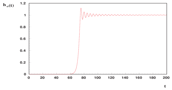
FIG. 12.: ${\cal F}(H/m)$ vs. $h$, where ${\cal F}(H/m)$ is defined by the relation $\phi_{eff}(t_{A})=(H/2\pi){\cal F}(H/m)$ (see eqs. (217) and (218)).

FIG. 13.: $\eta_{eff}^{2}(\tau)$ vs. $\tau$, for $\eta_{eff}(0)=3.94\times 10^{-7},\,\dot{\eta}_{eff}(0)=0.317\eta_{eff}(0),\,g=10^{-14},\,h_{0}=2.0$. The initial conditions were obtained by fitting the intermediate time regime of $g\Sigma(\tau)$ in fig.8. $\eta_{eff}(\tau)$ is the solution of eq.(219) with these initial conditions.

FIG. 14.: $h(\tau)$ vs. $\tau$, obtained from the solution of eqs. (219) and (221) with the conditions of fig.14.

Furthermore, this analysis shows that in the case $\eta=0$, the renormalized energy and pressure in this regime in which the renormalized integrals are dominated by the superhorizon modes are given by

$$\varepsilon_{R}(\tau)=\frac{2Nm^{4}_{R}}{\lambda_{R}}\left\{\frac{1}{2}\dot{\eta}^{2}_{eff}+\frac{1}{4}\left(-1+\eta^{2}_{eff}\right)^{2}\right\}\quad,\quad(p+\varepsilon)_{R}=\frac{2Nm^{4}_{R}}{\lambda_{R}}\left\{\dot{\eta}^{2}_{eff}\right\}$$ (220)

where we have neglected the contribution proportional to $1/a^{2}(\tau)$ because it is effectively red-shifted away after just a few e-folds. We found numerically that this term is negligible after the interval of time necessary for the superhorizon modes to dominate the contribution to the integrals. Then the dynamics of the scale factor is given by

$$h^{2}(\tau)=4h^{2}_{0}\left\{\frac{1}{2}\dot{\eta}^{2}_{eff}+\frac{1}{4}\left(-1+\eta^{2}_{eff}\right)^{2}\right\}\;.$$ (221)

We have numerically evolved the set of effective equations (219)-(221) by extracting the initial condition for the effective zero mode from the intermediate time behavior of $g\Sigma(\tau)$. We found a remarkable agreement between the evolution of $\eta^{2}_{eff}$ and $g\Sigma(\tau)$ and between the dynamics of the scale factor in terms of the evolution of $\eta_{eff}(\tau)$, and the full dynamics of the scale factor and quantum fluctuations within our numerical accuracy. Figs. 14 and 14 show the evolution of $\eta^{2}_{eff}(\tau)$ and $h(\tau)$ respectively from the classical evolution eqs. (219) and (221) using the initial condition $\eta_{eff}(\tau_{A})$ extracted from the exponential fit of $g\Sigma(\tau)$ in the intermediate regime. These figures should be compared to figs. 8 and 8. We have also numerically compared $p/\varepsilon$ given solely by the dynamics of the effective zero mode and it is again numerically indistinguishable from that obtained with the full evolution of the mode functions.

This is one of the main results of our work[15]. In summary: the modes that become superhorizon sized and grow through the spinodal instabilities assemble themselves into an effective composite zero mode a few e-folds after the beginning of inflation. This effective zero mode drives the dynamics of the FRW scale factor, terminating inflation when the non-linearities become important. In terms of the underlying fluctuations, the spinodal growth of superhorizon modes gives a non-perturbatively large contribution to the energy momentum tensor that drives the dynamics of the scale factor. Inflation terminates when the mean square root fluctuation probes the equilibrium minima of the tree level potential.

The extension of this analysis to the case for which $\eta(0)\neq 0$ is straightforward. Since both $\eta(\tau)$ and $\sqrt{g\Sigma(\tau)}=|C_{0}|f_{0}(\tau)$ obey the equation for the zero mode, eq.(150), it is clear that we can generalize our definition of the effective zero mode to be

$$\eta_{eff}(\tau)\equiv\sqrt{\eta^{2}(\tau)+g\Sigma(\tau)}\;.$$ (222)

which obeys the equation of motion of a classical zero mode:

$$\left[\frac{d^{2}}{d\tau^{2}}+3h(\tau)\frac{d}{d\tau}-1+\eta_{eff}(\tau)^{2}\right]\eta_{eff}(\tau)=0\;.$$ (223)

If this effective zero mode is to drive the FRW expansion, then the additional condition

$$\dot{\eta}_{eff}^{2}\;f_{0}^{2}-2\;\eta_{eff}\;\dot{\eta}_{eff}\;f_{0}\;\dot{f_{0}}+\eta_{eff}^{2}\;\dot{f_{0}}^{2}=\left[\dot{\eta}_{eff}\;f_{0}-\eta_{eff}\;\dot{f_{0}}\right]^{2}=0\;,$$ (224)

must also be satisfied. One can easily show that this relation is indeed satisfied if the mode functions factorize as in (212) and if the integrals in eqs.(215) are dominated by the contributions of the superhorizon mode functions. This leads to the conclusion that the gravitational dynamics is given by eqs. (220) – (221) with $\eta_{eff}(\tau)$ defined by (222). Eq.(224) is just the vanishing of the wronskian of $\eta_{eff}(\tau)$ and $f_{0}(\tau)$. Namely, $\eta_{eff}(\tau)$ and $f_{0}(\tau)$ just differ in a constant factor.

We see that in all cases, the full large $N$ quantum dynamics in these models of inflationary phase transitions is well approximated by the equivalent dynamics of a homogeneous, classical scalar field with initial conditions on the effective field $\eta_{eff}(\tau_{A})=\sqrt{g}\;h_{0}\;{\cal F}(h_{0})$. We have verified these results numerically for the field and scale factor dynamics, finding that the effective classical dynamics reproduces the results of the full dynamics to within our numerical accuracy. We have also checked numerically that the estimate for the classical to quantum crossover given by eq.(211) is quantitatively correct. Thus in the classical case in which $\eta(0)\gg\sqrt{g}\;h_{0}$ we find that $\eta_{eff}(\tau)=\eta(\tau)$, whereas in the opposite, quantum case $\eta_{eff}(\tau)=\sqrt{g\Sigma(\tau)}$.

This remarkable feature of zero mode assembly of long-wavelength, spinodally unstable modes is a consequence of the presence of the horizon. It also explains why, despite the fact that asymptotically the fluctuations sample the broken symmetry state, the equation of state is that of matter. Since the excitations in the broken symmetry state are massless Goldstone bosons one would expect radiation domination. However, the assembly phenomenon, i.e. the redshifting of the wave vectors, makes these modes behave exactly like zero momentum modes that give an equation of state of matter (upon averaging over the small oscillations around the minimum).

Subhorizon modes at the end of inflation with $q>h_{0}\,e^{h_{0}\tau_{s}}$ do not participate in the zero mode assembly. The behavior of such modes do depend on $q$ after the end of inflation. Notice that these modes have extremely large comoving $q$ since $h_{0}\,e^{h_{0}\tau_{s}}\geq 10^{26}$. As discussed in sec. VI such modes decrease with time after inflation as $\sim 1/a(\tau)$[13].

D Making sense of small fluctuations:

Having recognized the effective classical variable that can be interpreted as the component of the field that drives the FRW background and rolls down the classical potential hill, we want to recognize unambiguously the small fluctuations. We have argued above that after horizon crossing, all of the mode functions evolve proportionally to the zero mode, and the question arises: which modes are assembled into the effective zero mode whose dynamics drives the evolution of the FRW scale factor and which modes are treated as perturbations? In principle every $k\neq 0$ mode provides some spatial inhomogeneity, and assembling these into an effective homogeneous zero mode seems in principle to do away with the very inhomogeneities that one wants to study. However, scales of cosmological importance today first crossed the horizon during the last 60 or so e-folds of inflation. Recently Grishchuk[37] has argued that the sensitivity of the measurements of $\Delta T/T$ probe inhomogeneities on scales $\approx 500$ times the size of the present horizon. Therefore scales that are larger than these and that have first crossed the horizon much earlier than the last 60 e-folds of inflation are unobservable today and can be treated as an effective homogeneous component, whereas the scales that can be probed experimentally via the CMB inhomogeneities today must be treated separately as part of the inhomogeneous perturbations of the CMB.

Thus a consistent description of the dynamics in terms of an effective zero mode plus ‘small’ quantum fluctuations can be given provided the following requirements are met: a) the total number of e-folds $N_{e}\gg 60$, b) all the modes that have crossed the horizon before the last 60-65 e-folds are assembled into an effective classical zero mode via $\phi_{eff}(t)=\left[\phi^{2}_{0}(t)+\langle\pi^{2}(\vec{x},t)\rangle_{R}\right]^{\frac{1}{2}}$, c) the modes that cross the horizon during the last 60–65 e-folds are accounted as ‘small’ perturbations. The reason for the requirement a) is that in the separation $\phi(\vec{x},t)=\phi_{eff}(t)+\delta\phi(\vec{x},t)$ one requires that $\delta\phi(\vec{x},t)/\phi_{eff}(t)\ll 1$. As argued above, after the modes cross the horizon, the ratio of amplitudes of the mode functions remains constant and given by $e^{(\nu-\frac{3}{2})\Delta N}$ with $\Delta N$ being the number of e-folds between the crossing of the smaller $k$ and the crossing of the larger $k$. Then for $\delta\phi(\vec{x},t)$ to be much smaller than the effective zero mode, it must be that the Fourier components of $\delta\phi$ correspond to very large $k$’s at the beginning of inflation, so that the effective zero mode can grow for a long time before the components of $\delta\phi$ begin to grow under the spinodal instabilities. In fact requirement a) is not very severe; in the figs.8-11 we have taken $h_{0}=2.0$ which is a very moderate value and yet for $g=10^{-12}$ the inflationary stage lasts for well over 100 e-folds, and as argued above, the larger $h_{0}$ for fixed $g$, the longer is the inflationary stage. Therefore under this set of conditions, the classical dynamics of the effective zero mode $\phi_{eff}(t)$ drives the FRW background, whereas the inhomogeneous fluctuations $\delta\phi(\vec{x},t)$, which are made up of Fourier components with wavelengths that are much smaller than the horizon at the beginning of inflation and that cross the horizon during the last 60 e-folds, provide the inhomogeneities that seed density perturbations.

E Scalar Metric Perturbations:

Having identified the effective zero mode and the ‘small perturbations’, we are now in position to provide an estimate for the amplitude and spectrum of scalar metric perturbations. We use the clear formulation in ref.[38] in terms of gauge invariant variables. In particular we focus on the dynamics of the Bardeen potential[39], which in longitudinal gauge is identified with the Newtonian potential. The equation of motion for the Fourier components (in terms of comoving wavevectors) for this variable in terms of the effective zero mode is [eq.(4.48) in [38]]

$$\ddot{\Phi}_{k}+\left[H(t)-2\;\frac{\ddot{\phi}_{eff}(t)}{\dot{\phi}_{eff}(t)}\right]\dot{\Phi}_{k}+\left[\frac{k^{2}}{a^{2}(t)}+2\left(\dot{H}(t)-H(t)\;\frac{\ddot{\phi}_{eff}(t)}{\dot{\phi}_{eff}(t)}\right)\right]\Phi_{k}=0.$$ (225)

We are interested in determining the dynamics of $\Phi_{k}$ for those wavevectors that cross the horizon during the last 60 e-folds before the end of inflation. During the inflationary stage and substantially before its end the numerical analysis yields to a very good approximation

$$H(t)=H_{0}\;;\;\phi_{eff}(t)=\phi_{eff}(t_{A})\;e^{(\nu-\frac{3}{2})H_{0}(t-t_{A})},$$ (226)

where $H_{0}$ is the value of the Hubble constant during inflation, leading to

$$\Phi_{k}(t)=e^{(\nu-2)H_{0}(t-t_{A})}\left[a_{k}\;H^{(1)}_{\nu-1}\left(\frac{ke^{-H_{0}(t-t_{A})}}{H_{0}}\right)+b_{k}\;H^{(2)}_{\nu-1}\left(\frac{ke^{-H_{0}(t-t_{A})}}{H_{0}}\right)\right]\;\;.$$ (227)

The coefficients $a_{k},b_{k}$ are determined by the initial conditions and $\nu$ is given by eq.(190).

Since we are interested in the wavevectors that cross the horizon during the last 60 e-folds, the consistency for the zero mode assembly and the interpretation of ‘small perturbations’ requires that there must be many e-folds before the last 60. We are then considering wavevectors that were deep inside the horizon at the onset of inflation. $\Phi_{k}(t)$ is related to the canonical ‘velocity field’ that determines scalar perturbations of the metric and which is quantized with Bunch-Davies initial conditions for the large $k$-mode functions. The relation between $\Phi_{k}$ and $v$ and the initial conditions on $v$ lead at once to a determination of the coefficients $a_{k}$ and $b_{k}$ for $k>>H_{0}$ [see eqs.(13.5) and (13.9) in ref.[38]],

$$a_{k}={\dot{\phi}_{eff}(t_{A})\over k\;\sqrt{2H_{0}}\;M^{2}_{Pl}}\;e^{{i\pi\over 2}\left(\nu-\frac{3}{2}\right)}\;.$$ (228)

Thus we find that the amplitude of scalar metric perturbations after horizon crossing is given by

$$|\delta_{k}(t)|=k^{\frac{3}{2}}|\Phi_{k}(t)|={\dot{\phi}_{eff}(t_{A})\over\pi\;M^{2}_{Pl}}\,\Gamma(\nu-1)\;\left(\frac{2H_{0}}{k}\right)^{\nu-\frac{3}{2}}\;e^{(2\nu-3)H_{0}(t-t_{A})}\;.$$ (229)

The power spectrum per logarithmic $k$ interval is given by $|\delta_{k}(t)|^{2}$. The time dependence of $|\delta_{k}(t)|$ displays the unstable growth associated with the spinodal instabilities of super-horizon modes and is a hallmark of the phase transition. This time dependence can be also understood from the constraint equation that relates the Bardeen potential to the gauge invariant field fluctuations[38], which in longitudinal gauge are identified with $\delta\phi(\vec{x},t)$. The constraint equation and the evolution equations for the gauge invariant scalar field fluctuations are[38]

$$\frac{d}{dt}(a\Phi_{k})=\frac{4\pi}{M^{2}_{Pl}}\;a\;\delta\phi^{gi}_{k}\;\dot{\phi}_{eff}\;,$$ (230)

$$\left[\frac{d^{2}}{dt^{2}}+3H\frac{d}{dt}+\frac{k^{2}}{a^{2}}+{\cal M}^{2}\right]\delta\phi^{gi}_{k}-4\;\dot{\phi}_{eff}\;\dot{\Phi}_{k}+2V^{\prime}(\phi_{eff})\;\Phi_{k}=0\;.$$ (231)

Since the right hand side of (230) is proportional to $\dot{\phi}_{eff}/M^{2}_{Pl}\ll 1$ during the inflationary epoch in this model, we can neglect the terms proportional to $\dot{\Phi}_{k}$ and $\Phi_{k}$ on the left hand side of (231), in which case the equation for the gauge invariant scalar field fluctuation is the same as for the mode functions. In fact, since $\delta\phi^{gi}_{k}$ is gauge invariant we can evaluate it in the longitudinal gauge wherein it is identified with the mode functions $f_{k}(t)$. Then absorbing a constant of integration in the initial conditions for the Bardeen variable, we find

$$\Phi_{k}(t)=\frac{4\pi}{M^{2}_{Pl}\;a(t)}\int_{t_{o}}^{t}a(t^{\prime})\;\phi_{eff}(t^{\prime})\;f_{k}(t^{\prime})\;dt^{\prime}+{\cal O}\left(\frac{1}{M^{4}_{Pl}}\right),$$ (232)

and using that $\phi(t)\propto e^{(\nu-3/2)H_{0}t}$ and that after horizon crossing $f_{k}(t)\propto e^{(\nu-3/2)H_{0}t}$, one obtains at once the time dependence of the Bardeen variable after horizon crossing. In particular the time dependence is found to be $\propto e^{(2\nu-3)H_{0}t}$. It is then clear that the time dependence is a reflection of the spinodal (unstable) growth of the superhorizon field fluctuations.

To obtain the amplitude and spectrum of density perturbations at second horizon crossing we use the conservation law associated with the gauge invariant variable[38]

$$\xi_{k}=\frac{2}{3}\frac{\frac{\dot{\Phi}_{k}}{H}+\Phi_{k}}{1+p/\varepsilon}+\Phi_{k}\;\;;\;\;\dot{\xi}_{k}=0\;,$$ (233)

which is valid after horizon crossing of the mode with wavevector $k$. Although this conservation law is an exact statement of superhorizon mode solutions of eq.(225), we have obtained solutions assuming that during the inflationary stage $H$ is constant and have neglected the $\dot{H}$ term in Eq. (225). Since during the inflationary stage,

$$\dot{H}(t)=-\frac{4\pi}{M^{2}_{Pl}}\,\dot{\phi}^{2}_{eff}(t)\propto H^{2}_{0}\;\left(\frac{d\eta_{eff}(\tau)}{d\tau}\right)^{2}\ll H^{2}_{0}$$ (234)

and $\ddot{\phi}/\dot{\phi}\approx H_{0}$, the above approximation is justified. We then see that $\phi^{2}_{eff}(t)\propto e^{(2\nu-3)H_{0}t}$ which is the same time dependence as that of $\Phi_{k}(t)$. Thus the term proportional to $1/(1+p/\varepsilon)$ in Eq. (233) is indeed constant in time after horizon crossing. On the other hand, the term that does not have this denominator evolves in time but is of order $(1+p/\varepsilon)=-2\dot{H}/3H^{2}\ll 1$ with respect to the constant term and therefore can be neglected. Thus, we confirm that the variable $\xi$ is conserved up to the small term proportional to $(1+p/\varepsilon)\Phi_{k}$ which is negligible during the inflationary stage. This small time dependence is consistent with the fact that we neglected the $\dot{H}$ term in the equation of motion for $\Phi_{k}(t)$. The validity of the conservation law has been recently studied and confirmed in different contexts[40]. Notice that we do not have to assume that $\dot{\Phi}_{k}$ vanishes, which in fact does not occur.

However, upon second horizon crossing it is straightforward to see that $\dot{\Phi}_{k}(t_{f})\approx 0$. The reason for this assertion can be seen as follows: eq.(231) shows that at long times, when the effective zero mode is oscillating around the minimum of the potential with a very small amplitude and when the time dependence of the fluctuations has saturated (see fig.9), $\Phi_{k}$ will redshift as $\approx 1/a(t)$[13] and its derivative becomes extremely small.

Using this conservation law, assuming matter domination at second horizon crossing, and $\dot{\Phi}_{k}(t_{f})\approx 0$[38], we find

$$|\delta_{k}(t_{f})|={3\over 5\;\pi}{\Gamma(\nu)\over(\nu-\frac{3}{2})\,{\cal F}(H_{0}/m)}\left(\frac{2H_{0}}{k}\right)^{\nu-\frac{3}{2}}\;,$$ (235)

where ${\cal F}(H_{0}/m)$ determines the initial amplitude of the effective zero mode (218). We can now read the power spectrum per logarithmic $k$ interval

$${\cal P}_{s}(k)=|\delta_{k}|^{2}\propto k^{-2(\nu-\frac{3}{2})}.$$ (236)

leading to the index for scalar density perturbations

$$n_{s}=1-2\left(\nu-\frac{3}{2}\right)\;.$$ (237)

For $H_{0}/m\gg 1$, we can expand $\nu-3/2$ as a series in $m^{2}/H_{0}^{2}$ in eq.(235). Given that the comoving wavenumber of the mode which crosses the horizon $n$ e-folds before the end of inflation is $k=H_{0}\;e^{(N_{e}-n)}$ where $N_{e}$ is given by (209), we arrive at the following expression for the amplitude of fluctuations on the scale corresponding to $n$ in terms of the De Sitter Hubble constant and the coupling $\lambda=8\pi^{2}\,g$:

$$|\delta_{n}(t_{f})|\simeq\frac{9\,H^{3}}{10\,(2\pi)^{3/2}\,m^{3}}\left(2e^{n}\right)^{m^{2}/3H_{0}^{2}}\sqrt{\lambda}\left[1+\frac{2m^{2}}{3H_{0}^{2}}\left(\frac{7}{6}-\ln 2-\frac{\gamma}{2}\right)+{\cal O}\left(\frac{m^{4}}{H_{0}^{4}}\right)\right]\;.$$ (238)

Here, $\gamma$ is Euler’s constant. Note the explicit dependence of the amplitude of density perturbations on $\sqrt{g}$. For $n\approx 60$, the factor $\exp(nm^{2}/3H_{0}^{2})$ is ${\cal O}(100)$ for $H_{0}/m=2$, while it is ${\cal O}(1)$ for $H_{0}/m\geq 4$. Notice that for $H_{0}/m$ large, the amplitude increases approximately as $(H_{0}/m)^{3}$, which will place strong restrictions on $g$ in such models.

We remark that we have not included the small corrections to the dynamics of the effective zero mode and the scale factor arising from the non-linearities. We have found numerically that these nonlinearities are only significant for the modes that cross about 60 e-folds before the end of inflation for values of the Hubble parameter $H_{0}/m_{R}>5$. The effect of these non-linearities in the large $N$ limit is to slow somewhat the exponential growth of these modes, with the result of shifting the power spectrum closer to an exact Harrison-Zeldovich spectrum with $n_{s}=1$. Since for $H_{0}/m_{R}>5$ the power spectrum given by (237) differs from one by at most a few percent, the effects of the non-linearities are expected to be observationally unimportant. The spectrum given by (235) is similar to that obtained in references[4, 32] although the amplitude differs from that obtained there. In addition, we do not assume slow roll for which $(\nu-\frac{3}{2})\ll 1$, although this would be the case if $N_{e}\gg 60$.

We emphasize an important feature of the spectrum: it has more power at long wavelengths because $\nu-3/2>0$. This is recognized to be a consequence of the spinodal instabilities that result in the growth of long wavelength modes and therefore in more power for these modes. This seems to be a robust prediction of new inflationary scenarios in which the potential has negative second derivative in the region of field space that produces inflation.

It is at this stage that we recognize the consistency of our approach for separating the composite effective zero mode from the small fluctuations. We have argued above that many more than 60 e-folds are required for consistency, and that the small fluctuations correspond to those modes that cross the horizon during the last 60 e-folds of the inflationary stage. For these modes $H_{0}/k=e^{-H_{0}t^{*}(k)}$ where $t^{*}(k)$ is the time since the beginning of inflation of horizon crossing of the mode with wavevector $k$. The scale that corresponds to the Hubble radius today $\lambda_{0}=2\pi/k_{0}$ is the first to cross during the last 60 or so e-folds before the end of inflation. Smaller scales today will correspond to $k>k_{0}$ at the onset of inflation since they will cross the first horizon later and therefore will reenter earlier. The bound on $|\delta_{k_{0}}|\propto\Delta T/T\leq 10^{-5}$ on these scales provides a lower bound on the number of e-folds required for these type of models to be consistent:

$$N_{e}>60+\frac{12}{\nu-\frac{3}{2}}-\frac{\ln(\nu-\frac{3}{2})}{\nu-\frac{3}{2}}\;,$$ (239)

where we have written the total number of e-folds as $N_{e}=H_{0}\;t^{*}(k_{0})+60$. This in turn can be translated into a bound on the coupling constant using the estimate given by eq.(209).

The four year COBE DMR Sky Map[41] gives $n\approx 1.2\pm 0.3$ thus providing an upper bound on $\nu$

$$0\leq\nu-\frac{3}{2}\leq 0.05$$ (240)

corresponding to $h_{0}\geq 2.6$. We then find that these values of $h_{0}$ and $\lambda\approx 10^{-12}-10^{-14}$ provide sufficient e-folds to satisfy the constraint for scalar density perturbations.

F Tensor Metric Perturbations:

The scalar field does not couple to the tensor (gravitational wave) modes directly, and the tensor perturbations are gauge invariant from the beginning. Their dynamical evolution is completely determined by the dynamics of the scale factor[38, 42]. Having established numerically that the inflationary epoch is characterized by $\dot{H}/H^{2}_{0}\ll 1$ and that scales of cosmological interest cross the horizon during the stage in which this approximation is excellent, we can just borrow the known result for the power spectrum of gravitational waves produced during inflation extrapolated to the matter era[38, 42]

$${\cal P}_{T}(k)\approx\frac{H^{2}_{0}}{M^{2}_{Pl}}k^{0}\;.$$ (241)

Thus the spectrum to this order is scale invariant (Harrison-Zeldovich) with an amplitude of the order $m^{4}/\lambda M^{4}_{Pl}$. Then, for values of $m\approx 10^{12}-10^{14}\mbox{ Gev }$ and $\lambda\approx 10^{-12}-10^{-14}$ one finds that the amplitude is $\leq 10^{-10}$ which is much smaller than the amplitude of scalar density perturbations. As usual the amplification of scalar perturbations is a consequence of the equation of state during the inflationary epoch.

IX Conclusions

Since there are a number of articles in the literature treating related problems, it is useful to review the unique features of the present work. First, we have treated the problem dynamically, without using the effective potential (an equilibrium construct) to determine the evolution. Second, we have provided consistent non-perturbative calculations of the non-linear quantum field evolution to bring out some of the most relevant aspects of the late time behavior. In particular, we found that the quantum backreaction naturally inhibits catastrophic growth of fluctuations and provides a smooth transition to the late time regime in which the quantum fluctuations decay as the zero mode approaches its asymptotic state. Third, the dynamics studied obeys the constraint of covariant conservation of the energy momentum tensor.

It can be argued that the inflationary paradigm as currently understood is one of the greatest applications of quantum field theory. The imprint of quantum mechanics is everywhere, from the dynamics of the inflaton, to the generation of metric perturbations, through to the reheating of the universe. It is clear then that we need to understand the quantum mechanics of inflation in as deep a manner as possible so as to be able to understand what we are actually testing via the CMBR temperature anisotropies, say.

What we have found in our work is that the quantum mechanics of inflation is extremely subtle. We now understand that it involves both non-equilibrium as well as non-perturbative dynamics and that what you start from may not be what you wind up with at the end!

In particular, we see now that the correct interpretation of the non-perturbative growth of quantum fluctuations via spinodal decomposition is that the background zero mode must be redefined through the process of zero mode reassembly that we have discovered. When this is done (and only when!) we can interpret inflation in terms of the usual slow-roll approach with the now small quantum fluctuations around the redefined zero mode driving the generation of metric perturbations.

We have studied the non-equilibrium dynamics of a ‘new inflation’ scenario in a self-consistent, non-perturbative framework based on a large $N$ expansion, including the dynamics of the scale factor and backreaction of quantum fluctuations. Quantum fluctuations associated with superhorizon modes grow exponentially as a result of the spinodal instabilities and contribute to the energy momentum tensor in such a way as to end inflation consistently.

Analytical and numerical estimates have been provided that establish the regime of validity of the classical approach. We find that these superhorizon modes re-assemble into an effective zero mode and unambiguously identify the composite field that can be used as an effective expectation value of the inflaton field whose classical dynamics drives the evolution of the scale factor. This identification also provides the initial condition for this effective zero mode.

A consistent criterion is provided to extract small fluctuations that will contribute to cosmological perturbations from large non-perturbative spinodal fluctuations. This is an important ingredient for a consistent calculation and interpretation of cosmological perturbations. This criterion requires that the model must provide many more than 60 e-folds to identify the ‘small perturbations’ that give rise to scalar metric (curvature) perturbations. We then use this criterion combined with the gauge invariant approach to obtain the dynamics of the Bardeen variable and the spectrum for scalar perturbations.

We find that during the inflationary epoch, superhorizon modes of the Bardeen potential grow exponentially in time reflecting the spinodal instabilities. These long-wavelength instabilities are manifest in the spectrum of scalar density perturbations and result in an index that is less than one, i.e. a ‘red’ power spectrum, providing more power at long wavelength. We argue that this red spectrum is a robust feature of potentials that lead to spinodal instabilities in the region in field space associated with inflation and can be interpreted as an imprint of the phase transition on the cosmological background. Tensor perturbations on the other hand, are not modified by these features, they have much smaller amplitude and a Harrison-Zeldovich spectrum.

X Acknowledgements:

We thank F. Cao, D. Cormier, R. Holman, S. P. Kumar, J. Salgado, A. Singh, M. Srednicki all of whom collaborated at different stages on the works reviewed here. We thank J. Baacke, C. Destri, A. Dolgov, E. Kolb, E. Weinberg for conversations and discussions. D. B. thanks the N.S.F for partial support through the grant awards: PHY-9605186 and INT-9815064 and LPTHE for warm hospitality. We thank the CNRS-NSF cooperation programme for partial support.

REFERENCES

- [1] Laboratoire Associé au CNRS, UMR7589.
- [2] A. H. Guth, Phys. Rev. D23, 347 (1981).
- [3] For thorough reviews of standard and inflationary cosmology see: E. W. Kolb and M. S. Turner, The Early Universe (Addison Wesley, Redwood City, C.A. 1990). A. Linde, Particle Physics and Inflationary Cosmology, (Harwood 1990) and ref.[6].
- [4] For more recent reviews see: M. S. Turner, astro-ph-9703197; astro-ph-9703196; astro-ph-9703174; astro-ph-9703161; astro-ph-9704062; astro-ph-9704024. A. Linde, in Current Topics in Astrofundamental Physics, Proceedings of the Chalonge Erice School, N. Sánchez and A. Zichichi Editors, Nato ASI series C, vol. 467, 1995, Kluwer Acad. Publ. A. R. Liddle, astro-ph-9612093, Lectures at the Casablanca School Morocco, 1996.
- [5] G. Smoot, in the Proceedings of the Vth. Erice Chalonge School on Astrofundamental Physics, p. 407-484, N. Sánchez and A. Zichichi eds., World Scientific, 1997. A. R. Liddle and D. H. Lyth, Phys. Rep. 231, 1 (1993). A. E. Lange et al. , astro-ph/0005004, S. Hanany et al., astro-ph/0005123, P. de Bernardis et al., Nature 404 (2000) 955.
- [6] for reviews of inflation, see R. Brandenberger, Rev. of Mod. Phys. 57, 1 (1985); Int. J. Mod. Phys. A2, 77 (1987) and ref.[3].
- [7] D. Boyanovsky, D. Cormier, H. J. de Vega, R. Holman, S. P. Kumar, ‘Out of equilibrium fields in inflationary dynamics, density fluctuations’, in Proceedings of the NATO ASI ‘Current Topics in Astrofundamental Physics: Primordial Cosmology’, edited by N. Sánchez and A. Zichichi, vol C511, Kluwer Dordrecht, 1998.
- [8] D. Boyanovsky and H. J. de Vega, Phys. Rev. D47, 2343 (1993).
- [9] D. Boyanovsky, H. J. de Vega, R. Holman, D.-S. Lee and A. Singh, Phys. Rev. D51, 4419 (1995); D. Boyanovsky, M. D’Attanasio, H. J. de Vega, R. Holman and D. S. Lee, Phys. Rev. D52, 6805 (1995); For reviews see, D. Boyanovsky, H. J. de Vega and R. Holman, in the Proceedings of the Second Paris Cosmology Colloquium, Observatoire de Paris, June 1994, p. 127-215, H. J. de Vega and N. Sánchez Editors, World Scientific, 1995; D. Boyanovsky, M. D’Attanasio, H. J. de Vega, R. Holman and D.-S. Lee, ‘New aspects of reheating’, in the Proceedings of the Erice Chalonge School, ‘String Gravity and Physics at the Planck Energy Scale’, NATO ASI, N. Sánchez and A. Zichichi Editors, Kluwer 1996, p. 451-492.
- [10] D. Boyanovsky, H.J. de Vega, R. Holman, J.F.J. Salgado, Phys. Rev. D54, 7570 (1996). D. Boyanovsky, H. J. de Vega and R. Holman in the Proceedings of the Vth. Erice Chalonge School on Astrofundamental Physics, p. 183-270, N. Sánchez and A. Zichichi eds., World Scientific, 1997. D. Boyanovsky, C. Destri, H.J. de Vega, R. Holman and J.F.J. Salgado, Phys. Rev. D57, 7388 (1998).
- [11] D. Boyanovsky, H. J. de Vega, R. Holman and J. Salgado, Phys. Rev. D59, 125009 (1999).
- [12] D. Boyanovsky, H. J. de Vega, and R. Holman, Phys. Rev. D49, 2769 (1994).
- [13] D. Boyanovsky, D. Cormier, H. J. de Vega, R. Holman, A. Singh, M. Srednicki, Phys. Rev. D56, 1939 (1997).
- [14] D. Boyanovsky, D. Cormier, H. J. de Vega and R. Holman, Phys. Rev. D55, 3373 (1997).
- [15] D. Boyanovsky, D. Cormier, H. J. de Vega, R. Holman and S. P. Kumar, Phys. Rev. D57, 2166 (1998).
- [16] D. Boyanovsky, M. D’Attanasio, H. J. de Vega and R. Holman, Phys. Rev. D54, 1748 (1996), and references therein.
- [17] D. Boyanovsky and H. J. de Vega, Phys. Rev. D61, 105014 (2000).
- [18] D.T. Son, Phys. Rev. D54, 3745 (1996); hep-ph/9601377.
- [19] D.I. Kaiser, Phys. Rev D53, 1776 (1996), D56, 706 (1997) and D57, 702 (1998).
- [20] J. Schwinger, J. Math. Phys. 2, 407 (1961); P. M. Bakshi and K. T. Mahanthappa, J. Math. Phys. 4, 1 (1963); ibid, 12; L. V. Keldysh, Sov. Phys. JETP 20, 1018 (1965); A. Niemi and G. Semenoff, Ann. of Phys. (N.Y.) 152, 105 (1984); Nucl. Phys. B [FS10], 181 (1984); E. Calzetta, Ann. of Phys. (N.Y.) 190, 32 (1989); R. D. Jordan, Phys. Rev. D33, 444 (1986); N. P. Landsman and C. G. van Weert, Phys. Rep. 145, 141 (1987); R. L. Kobes and K. L. Kowalski, Phys. Rev. D34, 513 (1986); R. L. Kobes, G. W. Semenoff and N. Weiss, Z. Phys. C29, 371 (1985).
- [21] For non-equilibrium methods in cosmology see, for example: E. Calzetta and B.-L. Hu, Phys. Rev. D35, 495 (1988); ibid D37, 2838 (1988); J. P. Paz, Phys. Rev. D41, 1054 (1990); ibid D42, 529 (1990); B.-L. Hu in Bannf/Cap Workshop on TFT, ed. by F.C. Khanna, R. Kobes, G. Kunstatter, H. Umezawa, World Scientific, Singapore, 1994, p.309 and in the Proceedings of the Second Paris Cosmology Colloquium, Observatoire de Paris, edited by H. J. de Vega and N. Sánchez (World Scientific, Singapore, 1995), p.111 and references therein.
- [22] H. Leutwyler and S. Mallik, Ann. of Phys. (N.Y.) 205, 1 (1991).
- [23] O. Eboli, R. Jackiw and S.-Y. Pi, Phys. Rev. D37, 3557 (1988); M.Samiullah, O. Eboli and S-Y. Pi, Phys. Rev. D44, 2335 (1991). J. Guven, B. Liebermann and C. Hill, Phys. Rev. D39, 438 (1989).
- [24] N. D. Birrell and P.C.W. Davies, Quantum fields in curved space (Cambridge Univ. Press, Cambridge, 1986).
- [25] J. Baacke, K. Heitmann and C. Pätzold, Phys. Rev. D55, 2320 (1997), D56, 6556 (1997), D57, 6398 and 6406(1998).
- [26] M. Abramowitz and I.E. Stegun (eds.), Handbook of Mathematical Functions (National Bureau of Standards, Washington, D.C., 1972), chapter 13.
- [27] N. Turok, Ue-Li Pen, U. Seljak, Phys. Rev. D58, 023506 (1998). A. Albrecht, R. A. Battye, J. Robinson, Phys. Rev. Lett. 79, 4736 (1997). B. Allen, R. R. Caldwell, S. Dodelson, L. Knox, E. P. S. Shellard, A. Stebbins, Phys. Rev. Lett. 79, 2624 (1997). R. Durrer, astro-ph/0003363.
- [28] D. H. Lyth, hep-ph-9609431 (1996). S. Dodelson, W. H. Kinney and E. W. Kolb, Phys. Rev. D56, 3207 (1997).
- [29] A.D. Linde, Phys. Lett. B116, 335 (1982). A. Vilenkin and L. H. Ford, Phys. Rev. D26, 1231 (1982). A. Vilenkin, Nucl. Phys. B226, 504 (1983); Nucl. Phys. B226, 527 (1986).
- [30] A. Vilenkin, Phys. Lett. B115, 91 (1982).
- [31] P. J. Steinhardt and M. S. Turner, Phys. Rev. D29, 2162, (1984).
- [32] A. Guth and S-Y. Pi, Phys. Rev. D32, 1899 (1985).
- [33] For non-equilibrium methods in different contexts see for example: F. Cooper, J. M . Eisenberg, Y. Kluger, E. Mottola, B. Svetitsky, Phys. Rev. Lett. 67, 2427 (1991); F. Cooper, J. M. Eisenberg, Y, Kluger, E. Mottola, B. Svetitsky, Phys. Rev. D48, 190 (1993).
- [34] F. Cooper and E. Mottola, Mod. Phys. Lett. A 2, 635 (1987); F. Cooper, S. Habib, Y. Kluger, E. Mottola, J. P. Paz, P. R. Anderson, Phys. Rev. D50, 2848 (1994). F. Cooper, S.-Y. Pi and P. N. Stancioff, Phys. Rev. D34, 3831 (1986). F. Cooper and E. Mottola, Phys. Rev. D36, 3114 (1987). F. Cooper, Y. Kluger, E. Mottola, J. P. Paz, Phys. Rev. D51, 2377 (1995).
- [35] S. A. Ramsey, B. L. Hu, Phys. Rev. D56, 678 (1997).
- [36] D. Boyanovsky, H. J. de Vega and R. Holman, Phys. Rev. D 51, 734 (1995). D. Boyanovsky, H. J. de Vega, R. Holman and S. Prem Kumar, Phys. Rev. D56, 3929 and 5233 (1997). The last reference under [34]. J. Lesgourgues, D. Polarski and A. A. Starobinsky, Nucl. Phys. B497, 479 (1997).
- [37] L. P. Grishchuk, Phys. Rev. D 45, 4717 (1992).
- [38] V. F. Mukhanov, H. A. Feldman and R. H. Brandenberger, Phys. Rep. 215, 293 (1992).
- [39] J. Bardeen, Phys. Rev. D22, 1882 (1980).
- [40] R. R. Caldwell, Class. Quant. Grav. 13, 2437 (1995). J. Martin and D. J. Schwarz, Phys. Rev. D57 (1998) 3302.
- [41] K. M. Gorski, A. J. Banday, C. L. Bennett, G. Hinshaw, A. Kogut and G. F. Smoot, astro-ph-9601063.
- [42] L. P. Grishchuk, Phys. Rev. D. 52, 5549, (1995); Proceedings of the Erice Chalonge School NATO ASI on ‘String Gravity and Physics at the Planck Scale’, Ed. N. Sánchez and A. Zichichi, (Kluwer, 1996), p. 369; Phys. Rev. D53 (1996) 6784; Proceedings of the NATO ASI on ‘Current Topics in Astrofundamental Physics’, Ed. N. Sanchez and A. Zichichi (Kluwer, 1995), p. 205. Rev. Mod. Phys. 69, 373, (1997).
- [43] I. Zlatev, G. Huey and P. J. Steinhardt, Phys. Rev. D 57, 2152 (1998).
- [44] F. Cooper, S. Habib, Y. Kluger, E. Mottola, J. P. Paz, and P. R. Anderson, Phys. Rev. D50, 2848 (1994).
- [45] J. Avan and H. J. de Vega, Nucl. Phys. B224, 61 (1983). M. B. Halpern, Nucl. Phys. B 173, 504 (1980).
- [46] D. Boyanovsky, H. J. de Vega, R. Holman, S. Prem Kumar and R. D. Pisarski, Phys. Rev. D57, 3653 (1998). F. J. Cao and H. J. de Vega, hep-ph/9911537.