Double Inflation in Supergravity and the Boomerang Observations

Abstract

One of the biggest mystery of the recent observation of cosmic microwave background anisotropies by the boomerang team is insignificance of the second acoustic peak in the angular power spectrum. It is very difficult to explain such a low amplitude without assuming the higher baryon density than predicted by the Big Bang Nucleosynthesis (BBN). Employing the double inflation model in supergravity, we show that the density fluctuations produced by this inflation model can produce a sufficient low second acoustic peak with the standard value of the baryon density from BBN. It is shown that these density fluctuations are also consistent with the observations of cluster abundances and galaxy distributions.

]

I Introduction

After the discovery by COBE/DMR [1], anisotropies of Cosmic Microwave Background radiation (CMB) become one of the most important targets of modern cosmology. Theoretical works reveal that they contain rich information, i.e., geometry of the universe, the baryon density, the total matter density, the Hubble parameter, thermal history and so on [2]. However, it turns out that the angular resolution of COBE/DMR was too crude to obtain above information. Precise measurements of so-called acoustic peaks in the angular power spectrum on arcminute scales are necessary to determine these cosmological parameters.

There are many attempts to observe CMB anisotropies on arcminute scales after COBE/DMR discovery[3]. Recently, the boomerang team has reported very clear evidence of the first acoustic peak in the angular power spectrum of CMB anisotropies [4]. The location of the peak suggests the flatness of the universe. However, there remain some mysteries in their result. One of them is a relatively low second acoustic peak if there exists. The most natural way to explain such a low peak is to increase the value of $\Omega_{B}h^{2}$, where $\Omega_{B}$ is the baryon density parameter and $h$ is the non-dimensional Hubble constant normalized by $100\rm km/s/Mpc$, since increasing $\Omega_{B}h^{2}$ boosts only odd number peaks [2]. In order to fit the data, however, $\Omega_{B}h^{2}$ needs to be larger than the value constrained by Big Bang Nucleosynthesis (BBN) [5].

There are several possibilities to explain the low amplitude of the second acoustic peak. Among them, a tilted initial power spectrum, increasing the diffusion length [6], and degenerated neutrinos [7] can be considered. However, it seems that none of them provides a small enough second-first peak height ratio without increasing $\Omega_{B}h^{2}$. Here we propose double inflation which breaks a coherent feature of the initial power spectrum as a candidate for solving this mystery.

Recently we studied a double inflation model with hybrid and new inflations and its cosmological implication [8]. It was found that both inflations could produce cosmologically relevant density fluctuations if the total $e$-fold number of new inflation is small enough. In this case, there appears a breaking scale in the density power spectrum which corresponds to the horizon scale of the transit epoch from hybrid to new inflation. The fluctuations on scales larger (smaller) than the breaking are produced by hybrid (new) inflation. Assuming the ’standard’ cold dark matter model with $\Omega_{0}=1$, where $\Omega_{0}$ is the density parameter of a matter component, we can fit both cluster abundances and galaxy distributions with the COBE/DMR normalization when we set the amplitude of perturbations produced by new inflation is smaller than the one by hybrid inflation. Accordingly we generally obtain smaller acoustic peaks in the CMB angular power spectrum since the peaks are controlled by new inflation and the Sachs-Wolfe tail on larger scales whose amplitude is fixed by the COBE normalization is determined by hybrid inflation.

Therefore, we may be able to explain cluster abundances, galaxy distributions and the low second acoustic peak at once by introducing double inflation if the braking scale is in between first and second peaks by chance. In this paper, we first explain the double inflation model and compare the resultant density power spectrum and CMB angular power spectrum with observational data. We take $\Omega_{0}+\lambda_{0}=1$, i.e., a spatially flat universe. Here $\lambda_{0}$ is the density parameter of a cosmological constant. We also take $\Omega_{B}h^{2}=0.02$ which is the best value from BBN analysis [9].

II Double inflation model

We adopt a double inflation model proposed in Ref.[10]. Here we briefly describe the model in order to show the relation between model parameters and the power spectrum of the density fluctuations. The model consists of two inflationary stages; the first one is called preinflation. Here we employ hybrid inflation [11] (see also Ref.[12]) as preinflation. We also assume that the second inflationary stage is realized by a new inflation model [13] and its $e$-fold number is smaller than $\sim 60$. Thus, the density fluctuations on large scales are produced during preinflation and their amplitudes should be normalized to the COBE data [14]. On the other hand, new inflation produces fluctuations on small scales. Thus, this power spectrum has a break on the scale corresponding to a turning epoch from preinflation to new inflation. As for the detailed argument of dynamics of our model, see Refs. [8, 16, 17].

A First inflationary stage

First, let us briefly discuss a hybrid inflation model [11]. The hybrid inflation model contains two kinds of superfields: one is $S(x,\theta)$ and the others are a pair of $\Psi(x,\theta)$ and $\bar{\Psi}(x,\theta)$. Here $\theta$ is the Grassmann number denoting superspace. The model is based on the U$(1)_{R}$ symmetry under which $S(\theta)\rightarrow e^{2i\alpha}S(\theta e^{-i\alpha})$ and $\Psi(\theta)\bar{\Psi}(\theta)\rightarrow\Psi(\theta e^{-i\alpha})\bar{\Psi}(\theta e^{-i\alpha})$. The superpotential is given by [11]

$$W(S,\Psi,\bar{\Psi})=-\mu^{2}S+\lambda S\bar{\Psi}\Psi.$$ (1)

The $R$-invariant Kähler potential is given by

$$K(S,\Psi,\bar{\Psi})=|S|^{2}+|\Psi|^{2}+|\bar{\Psi}|^{2}+\cdots,$$ (2)

where the ellipsis denotes higher-order terms which we neglect in the present analysis for simplicity. We gauge the U$(1)$ phase rotation:$\Psi\rightarrow e^{i\delta}\Psi$ and $\bar{\Psi}\rightarrow e^{-i\delta}\bar{\Psi}$. To satisfy the $D$-term flatness condition we take always $\Psi=\bar{\Psi}$ in our analysis. For $|S|>|S_{c}|=\mu/\sqrt{\kappa}$, the effective potential $V$ has a minimum at $\Psi=\bar{\Psi}=0$. That is, for $|S|>|S_{c}|$, the energy density is dominated by the false vacuum energy density $\mu^{4}$ and inflation takes place. We identify the inflaton field $\sigma/\sqrt{2}$ with the real part of the field $S$.

We define $N_{\rm COBE}$ as the $e$-fold number corresponding to the COBE scale and the COBE normalization leads to a condition for the inflaton potential,

$$\left|\frac{V^{3/2}}{V^{\prime}}\right|_{N_{\rm COBE}}\simeq\frac{4\pi\mu^{2}\sqrt{N_{\rm COBE}}}{\lambda}\simeq 5.3\times 10^{-4},$$ (3)

where $V$ is the inflaton potential obtained from Eqs.(1) and (2) including one-loop corrections. In the hybrid inflation model, density fluctuations are almost scale invariant, $n_{\rm pre}\simeq 1$, where $n_{\rm pre}$ is a spectral index for a power spectrum of density fluctuations.

B Second inflationary stage

Now, we consider a new inflation model. We adopt an inflation model proposed in Ref. [13]. The inflaton superfield $\phi(x,\theta)$ is assumed to have an $R$ charge $2/(n+1)$ and U$(1)_{R}$ is dynamically broken down to a discrete $Z_{2nR}$ at a scale $v$, which generates an effective superpotential [13, 10],

$$W(\phi)=v^{2}\phi-\frac{g}{n+1}\phi^{n+1}.$$ (4)

The $R$-invariant effective Kähler potential is given by

$$K(\phi)=|\phi|^{2}+\frac{\kappa}{4}|\phi|^{4}+\cdots,$$ (5)

where $\kappa$ is a constant of order $1$. Hereafter we take $n=4$ and $g=1$ for simplicity.

An important point on the density fluctuations produced by new inflation is that it results in a tilted spectrum with spectral index $n_{\rm new}$ given by

$$n_{\rm new}\simeq 1-2\kappa.$$ (6)

C Initial value and fluctuations of the inflaton $\varphi$

The crucial point observed in Ref. [10] is that preinflation sets dynamically the initial condition for new inflation. We identify the inflaton field $\varphi(x)/\sqrt{2}$ with the real part of the field $\phi(x)$. Then, the value of $\varphi$ at the beginning of new inflation is given by [17]

$$\varphi_{b}\simeq\frac{\sqrt{2}}{\sqrt{\lambda}}v\left(\frac{v}{\mu}\right)^{2}.$$ (7)

Therefore, in our model, $\varphi_{b}$, the $e$-fold number of the second inflation ($N_{\rm new}$), and $N_{\rm COBE}$ are determined by only model parameters. On the contrary, in the other double inflation models $\varphi_{b}$ should be put by hand. In our model we have four model parameters $(\mu,\lambda,v,\kappa)$ among which $\mu$ is expressed by the other parameters with use of Eq. (3). Thus there are three free parameters.

D Numerical results

We estimate density fluctuations in double inflation by calculating the evolution of $\varphi$ and $\sigma$ numerically. For given parameters $\kappa$ and $\lambda$, we obtain the breaking scale $k_{b}$ and the amplitude of the density fluctuations $\delta_{b}$ produced at the beginning of new inflation. Here, $k_{b}^{-1}$ is the comoving breaking scale corresponding to the Hubble radius at the beginning of new inflation. We can understand the qualitative dependence of $(k_{b},\delta_{b})$ on $(\kappa,\lambda)$ as follows: When $\kappa$ is large, the slope of the potential for new inflation is too steep, and new inflation cannot last for a long time. Therefore, the break occurs at smaller scales. In fact, we can express $k_{b}$ as

$$k_{b}\sim\frac{1}{3000}h{\rm Mpc}^{-1}\exp\left[50-\frac{1}{\kappa}\ln\left(\sqrt{\frac{\lambda(1-\kappa)}{12}}\frac{\mu^{2}}{v^{2}}\right)\right].$$ (8)

As for $\delta_{b}$, we can see from Eq.(3) that as $\lambda$ becomes larger, $\mu$ also must become larger. In addition, we can show that

$$\delta_{b}\equiv\left(\frac{\delta\rho}{\rho}\right)_{{\rm new},k_{b}}\simeq\frac{1}{5\sqrt{6}\pi}\frac{\sqrt{\lambda}\mu^{2}}{\kappa v},$$ (9)

for a given $v$ (see Ref. [8]). Thus, we have larger $\delta_{b}$ for larger $\lambda$.

In our previous work [8], we have shown that if $\lambda\sim{\cal O}(10^{-4}-10^{-3})\quad{\rm and}\quad 0.1\lesssim\kappa\lesssim 0.2$ , $k_{b}$ is at a cosmological scale ($10^{-3}h{\rm Mpc^{-1}}\lesssim k_{b}\lesssim 1h{\rm Mpc^{-1}}$), and density fluctuations produced during new inflation are not too far from those of preinflation ($0.1\lesssim{\cal R}\equiv P_{\rm new}/P_{\rm pre}\lesssim 10$). Here $P_{\rm new}$ and $P_{\rm pre}$ refer to the amplitude of the power spectrum of the density fluctuations at $k_{b}$, produced by new inflation and preinflation, respectively:

$$P(k)=\left\{\begin{array}[]{l}P_{\rm pre}\left(\frac{k}{k_{b}}\right)^{1}T^{2}(k)\quad(k<k_{b}),\\ P_{\rm new}\left(\frac{k}{k_{b}}\right)^{n_{\rm new}}T^{2}(k)\quad(k>k_{b}),\end{array}\right.$$ (10)

where $T(k)$ is a matter transfer function.

III Comparison with observations

A Second acoustic peak

The spectral index of new inflation $n_{\rm new}$ is $n_{\rm new}\simeq 1-2\kappa<1$ [see Eq.(6)]. Also, the amplitude of the density fluctuations on smaller scales, which are produced during new inflation, can be smaller than that on larger scales, which is normalized to the COBE/DMR data. Thus, in our double inflation model, if the breaking scale $k_{b}$ is in between the first and the second peaks of the CMB angular power spectrum, there is a possibility to explain the lower second acoustic peak of the boomerang results.

Here we take $n_{\rm new}\simeq 0.8\ (\kappa\simeq 0.1)$ as an example. Since the location of the first acoustic peak (the multipole moment $\ell\sim 200$) corresponds to the comoving wave number $k\sim{\cal O}(10^{-2})h$Mpc^-1, we have searched parameter sets within the parameter range of $0.001h{\rm Mpc}^{-1}\lesssim k_{b}\lesssim 0.04h{\rm Mpc}^{-1}$, and $0.7\lesssim{\cal R}\lesssim 1$, which can produce a lower second acoustic peak of the CMB angular power spectrum.

In Table I, samples of these parameters are listed. From the recent observations of Type Ia supernovae, $\Omega_{0}$ is estimated as $\Omega_{0}\lesssim 0.5$ [18]. Therefore, we take $\Omega_{0}=0.4,0.5,$ and $0.6$, for example. Also, in Fig.1, we plot the angular power spectrum of the CMB anisotropies for these parameters. From this figure, we can see that our double inflation model has a parameter region which can explain the lower second acoustic peak of the boomerang observations as expected.

B Cluster abundances and galaxy distribution

As we have seen in the previous subsection, our double inflation model can explain the low second acoustic peak of the boomerang data. However, we need to check whether it is consistent with other observations. In this subsection we compare the result of our double inflation model with the observations of the cluster abundances [19, 20] and galaxy distributions [21].

Usually the constraint on the power spectrum from observations of the cluster abundances is expressed in terms of $\sigma_{8}$, the specific mass fluctuations within a sphere of a radius of $8h^{-1}\rm Mpc$. Since the power spectrum of the density fluctuations shows a break on the cosmological scale in our double inflation model, we cannot simply employ the value of $\sigma_{8}$ quoted by previous works [19, 20]. We need to calculate the cluster abundances by using the Press-Schechter theory [22].

When we determine the breaking scale $k_{b}$, the power spectrum ratio ${\cal R}\equiv P_{\rm new}/P_{\rm pre}$, and the spectral index for new inflation $n_{\rm new}$, we can get the power spectrum up to normalization $A_{\rm cl}$. Using this power spectrum we can calculate the comoving abundance of the clusters as

$$n(>M_{\rm min};A_{\rm cl})=\int^{\infty}_{M_{\rm min}}\frac{dn(M)}{dM}dM,$$ (11)

where mass distribution $dn/dM$ is obtained by the Press-Schechter formula.

Many clusters of galaxies are observed with use of x-ray fluxes. Under the assumption that clusters are hydrostatic, we can obtain the mass-temperature relations as

$$T_{\rm gas}=\frac{9.37\ {\rm keV}}{\beta(5X+3)}\left(\frac{M}{10^{15}h^{-1}M_{\odot}}\right)^{2/3}(1+z)\Omega_{0}^{1/3}\Delta_{c}^{1/3},$$ (12)

where $\Delta_{c}$ is the ratio of the density of a cluster to the background mean density at that redshift, $\beta$ is the ratio of specific galaxy kinetic energy to specific gas thermal energy, and $X$ is the hydrogen mass fraction. Following Ref. [19], we take $X=0.76$, $\beta=1$. Also, $\Delta_{c}$ can be approximated as $\Delta_{c}\simeq 18\pi^{2}\left[1+0.4093\left(1/\Omega_{0}-1\right)^{0.9052}\right]$ [23].

The observed cluster abundance as a function of x-ray temperature can be translated into a function of mass using Eq. (12). Accumulating the observations, Henry and Arnaud [24] gave the fitting formula as

$$\left(\frac{dn(T)/dT}{h^{3}{\rm Mpc}^{-3}{\rm keV}^{-1}}\right)=1.8\left\{\begin{array}[]{l}+0.8\\ -0.5\end{array}\right\}\times 10^{-3}\left(\frac{kT}{1{\rm keV}}\right)^{-4.7\pm 0.5}.$$ (13)

Ref. [24] also gave a table of cluster observations whose temperatures are larger than $2.5$ keV, which determines the lower limit $M_{\rm min}$ from Eq. (12). Therefore, by integrating Eq. (13) we obtain

$$6.6\times 10^{-6}\ \lesssim\ n(>M_{\rm min})\ \lesssim\ 4.3\times 10^{-5}.$$ (14)

Matching these abundances, Eq. (11) calculated from the Press-Schechter theory, and Eq. (14) inferred from the x-ray cluster observations, we can determine the normalization (amplitude) of power spectrum, $A_{\rm cl}$. Using this normalization, we can obtain “cluster abundance normalized” $\sigma_{8}$, $\sigma_{\rm 8,cl}$, as

$$\left.\sigma_{\rm 8,cl}^{2}\equiv\int^{\infty}_{0}\frac{k^{3}}{2\pi^{2}}P(k;A_{\rm cl})W^{2}(kr_{0})\frac{dk}{k}\right|_{r_{0}=8h^{-1}{\rm Mpc}}.$$ (15)

where $P(k;A)$ is a present matter density fluctuation power spectrum with a normalization $A$, and $W(x)$ is a window function. Because of errors in observations, we have some range for allowed $\sigma_{\rm 8,cl}$.

On the other hand, we can normalize the power spectrum by COBE data [14, 25]. Therefore, we have “COBE normalized” $\sigma_{8}$, $\sigma_{\rm 8,COBE}$ together with $\sigma_{\rm 8,cl}$. Bunn and White [25] estimates one standard deviation error of COBE normalization to be $7\%$ which is much smaller than the one of cluster normalization. We assume that, therefore, if $\sigma_{\rm 8,COBE}$ lies in an allowed $\sigma_{\rm 8,cl}$ range, the parameter region of $k_{b}$, ${\cal R}$, and $n_{\rm new}$ is consistent with the cluster abundance observations. As for the parameter sets for models (a) to (c) in Table I, we have confirmed that they all satisfy the cluster abundance constraint.

We also have to investigate whether our parameter sets are consistent with the observations of galaxy distributions. There are many observations which measure the density fluctuations from galaxy distributions. Among them we use the data sets compiled by Vogeley [26] from Refs. [21] in this paper.

Employing the COBE normalization, we can determine the power spectrum with its overall amplitude if we fix the breaking scale $k_{b}$, the power spectrum ratio ${\cal R}$, and the spectral index for new inflation $n_{\rm new}$. One might make direct comparison of this power spectrum with above observations of galaxy distributions. However, distribution of luminous objects such as galaxies could differ from underlying mass distribution because of so-called bias. There is even no guarantee that each observational sample has the same bias factor. Therefore, we only consider the shape of the power spectrum here. We change the overall amplitude of each set of observations arbitrarily. Thus, we estimate the goodness of fitting by calculating $\chi^{2}$ of this power spectrum with fixing $k_{b},{\cal R}$, and $n_{\rm new}$.

For each parameter set we have chosen in the previous subsection, they fit the observations of galaxy distributions well (reduced $\chi^{2}_{\rm gal}\simeq 1$), except for model (a) [see Table I]. In Fig. 2, we plot the power spectrum of the density fluctuations for the model (b) in Table I as an example.

IV Conclusions and discussions

The boomerang team has reported that there is a low second acoustic peak in the angular power spectrum of CMB anisotropies. Although there are some explanations to this lower peak, they seem to need higher baryon density than predicted by the Big Bang Nucleosynthesis. In this paper, we have considered the double inflation model in supergravity, and shown that the density fluctuations produced by this inflation model can produce this low second acoustic peak.

Since the density fluctuations in our model has a nontrivial spectrum, we have checked that it is consistent with the observations of the cluster abundances and the galaxy distributions. We have found that the fit to the data in our model is very good if we take $\Omega_{0}\simeq 0.5$. We can conclude that the double inflation model can account for the boomerang data without conflicting other observations. In particular, we stress that our model does not require high baryon density and hence is perfectly consistent with BBN.

T. K. is grateful to K. Sato for his continuous encouragement. A part of this work is supported by Grant-in-Aid of the Ministry of Education and by Grant-in-Aid, Priority Area “Supersymmetry and Unified Theory of Elementary Particles” (#707).

TABLE I.: The break parameters and reduced $\chi^{2}_{\rm gal}$. In the models (a) to (c), we employ $n_{\rm new}=0.8$. For comparison, the cosmological constant dominated CDM model and the ’standard’ standard CDM model are shown in (d) and (e), respectively. In all cases, $\Omega_{B}h^{2}=0.02$.

model	$\Omega_{0}$	$h$	$k_{b}[h{\rm Mpc}^{-1}]$	${\cal R}$	reduced $\chi^{2}_{\rm gal}$
(a)	0.4	0.7	0.025	0.78	1.65
(b)	0.5	0.65	0.034	0.76	1.09
(c)	0.6	0.6	0.032	0.80	0.77
(d)	0.4	0.7	$\cdots$	1.00	0.61
(e)	1.0	0.5	$\cdots$	1.00	1.51

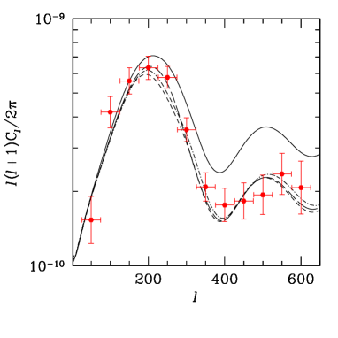
FIG. 1.: The CMB angular power spectra for four parameter sets. The symbols with error bars are the boomerang data. The short dash line, long dash line, and dot-short dash line correspond to model (a) to (c) in Table I, respectively. For comparison, we also plot the Lambda CDM model (model (d) in Table I) in a solid line.

FIG. 2.: The power spectrum of the density fluctuations for the model (b) in Table I.

REFERENCES

- [1] G. Smoot et al., Astrophys. J. 396, L1 (1992).
- [2] W. Hu, N. Sugiyama, and J. Silk, Nature 386, 37 (1997)
- [3] see e.g., Max Tegmark’s home page, http://www.hep.upenn.edu/ max/cmb/experiments.html
- [4] P.de Bernardis et al., Nature 404, 955 (2000).
- [5] A. E. Lange et al., astro-ph/0005004.
- [6] M. White, D. Scott, and E. Pierpaol, astro-ph/0004385.
- [7] J. Lesgourgues,and M. Peloso, astro-ph/0004412; S. Hannestad, astro-ph/0005018; M. Orito, T. Kajino, G. J. Mathews and R. N. Boyd, astro-ph/0005446.
- [8] T. Kanazawa, M. Kawasaki, N. Sugiyama, and T. Yanagida, Phys. Rev. D61, 023517 (2000).
- [9] K. A. Olive, G. Steigman and T. P. Walker, astro-ph/9905320 (submitted to Phys. Rep.).
- [10] K.I. Izawa, M. Kawasaki and T. Yanagida, Phys. Lett. B411, 249 (1997).
- [11] G. Dvali, Q. Shafi, and R. K. Shaefer, Phys. Rev. Lett. 73, 1886 (1994); E. J. Copeland, A. R. Liddle, D. H. Lyth, E. D. Stewart, and D. Wands, Phys. Rev. D49, 6410 (1994).
- [12] C. Panagiotakopolous, Phys. Rev. D55, 7335 (1997); A. Linde and A. Riotto, Phys. Rev. D56, R1841 (1997).
- [13] K.I. Izawa and T. Yanagida, Phys. Lett. B393, 331 (1997); K. Kumekawa, T. Moroi and T. Yanagida, Prog. Theor. Phys. 92, 437 (1994).
- [14] C.L. Bennett et al., Astrophys. J. 464, L1 (1996).
- [15] M. White, D. Scott, J. Silk and M. Davis, Mon. Not. R. Astron. Soc. 276, L69 (1995).
- [16] M. Kawasaki, N. Sugiyama and T. Yanagida, Phys. Rev. D57, 6050 (1998).
- [17] M. Kawasaki and T. Yanagida, Phys. Rev. D59, 043512 (1999).
- [18] S. Perlmutter et al., Astrophys. J. 517, 565 (1999).
- [19] V. Eke, S. Cole, and C. S. Frenk, Mon. Not. R. Astron. Soc. 282, 263 (1996).
- [20] P. T. P. Viana and A. R. Liddle, in Proceedings of the Conference “Cosmological Constraints from X-Ray Clusters”, astro-ph/9902245.
- [21] L. N. da Costa et al., Astrophys. J. 437, L1 (1994); H. Lin et al., Astrophys. J. 471, 617 (1996); K. B. Fisher et al., Astrophys. J. 402, 42 (1993); H. A. Feldman, N. Kaiser, and J. A. Peacock, Astrophys. J. 426, 23 (1994); H. Tadros and G. Efstathiou, Mon. Not. R. Astron. Soc. 276, L45 (1995).
- [22] W. H. Press and P. Schechter, Astrophys. J. 187, 425 (1974).
- [23] T. T. Nakamura and Y. Suto, Prog. Theor. Phys. 97, 49 (1997).
- [24] J. P. Henry and K. A. Arnaud, Astrophys. J. 372, 410 (1991).
- [25] E. F. Bunn and M. White, Astrophys. J. 480, 6 (1997)
- [26] M. S. Vogeley, in The Evolving Universe, edited by D. Hamilton (Kluwer, Dordrecht, 1998), p.395.